Abstract
The decentralization and anonymity of blockchain have attracted significant attention. However, in recent years, there has been a rise in blockchain money laundering incidents, and anti-money laundering efforts have become crucial within the blockchain space. Blockchain money laundering differs from traditional financial money laundering as it does not provide account information, particularly in the case of Bitcoin. This absence of information makes it challenging for researchers to detect money laundering activities based on transaction data. We propose LB-GLAT, a novel Long-Term Bi-Graph Layer Attention Convolutional Network, to effectively capture the topological structure and attribute characteristics of money laundering on the blockchain transaction graph. LB-GLAT utilizes the transaction graph and the reverse transaction graph to solve the no-loop problem that results in the inability to capture the destination of blockchain transactions and designs a long-term layer attention mechanism to alleviate the over-smoothing problem. We implemented a series of experiments to evaluate LB-GLAT, which achieved state-of-art performance compared with other methods, presenting an accuracy of 0.9776, a precision of 0.9317, a recall of 0.8494, an F1−score of 0.8887, and an AUC of 0.9806.
MSC:
68T07; 68T30
1. Introduction
Blockchain has become a hot topic due to its decentralized, immutable, and anonymous characteristics [1]. However, the anonymity of blockchain has also hindered government and market regulation, leading to increasing illegal activities among criminals using blockchain to launder money [2]. Money launderers use funds obtained from illicit activities, such as gambling, drug trafficking, and Ponzi schemes, to purchase cryptocurrencies for trading on the blockchain, which are converted into legitimate funds [3]. The blockchain intelligence and forensics company CipherTrace reported that the global amount of bitcoin used in crimes has reached USD 4.5 billion [4]. Chainalysis, an American blockchain analysis firm headquartered in New York City, reported that illicit addresses sent nearly USD 23.8 billion worth of cryptocurrency in 2022, a 68.0% increase compared to 2021 [5]. Blockchain money laundering is becoming more and more rampant. Cryptocurrencies such as Bitcoin have become a paradise for financial criminals [6].
Currently, international organizations and governments are focusing on blockchain money laundering. They want to strengthen supervision to curb the occurrence of money laundering crimes. For example, the Financial Action Task Force updated its report on the implementation of standards on virtual assets and virtual asset service providers in 2021, calling on countries to strengthen the regulation of virtual assets [7]. Furthermore, the European Union agreed on the cryptocurrency regulation protocol “Markets in Crypto-assets” in 2022, which regulates market participants, including trading platforms [8].
Academics, meanwhile, are also paying attention to the topic. The research methods are divided into two main categories for anti-money laundering: traditional machine learning methods and deep learning methods. Some researchers have used traditional machine learning methods to detect money laundering activities, such as random forest [9], K-means Clustering [10], and Gaussian mixture models [11]. However, these methods face serious challenges, such as limited parameters, which may lead to suboptimal performance and difficulty capturing the transaction topology structure the hides blockchain money laundering features. Therefore, more and more researchers are focusing on deep learning methods to solve these problems, especially graph convolutional neural networks (GCNs) and their variations, which can thoroughly learn the graph topology to improve detection accuracy further. For example, Weber et al. [12] assessed the detection effect of a GCN model trained on the Ellipse dataset. Alarab et al. [13] proposed graph convolutional networks interwoven with a GCN and linear layers for modeling. It is noteworthy that, in contrast to the user/account graph of the traditional financial field, these researchers mostly employed a transaction graph. This graph represents transactions as nodes and the flow of transaction funds as edges, serving as a foundation for detecting money laundering in UTXO-based (unspent transaction output) blockchains. This stems from the inherent nature of UTXO-based blockchains, which do not maintain records of account information and balances. Furthermore, constructing the user/account graph using alternative identifiers like public keys or wallet addresses is nearly infeasible. Firstly, public keys are not directly stored on the blockchain. Instead, their hash values are recorded. However, it is worth noting that the hash value of the same user’s or wallet’s public key may vary. Secondly, wallet data concerning UTXO-based blockchains are typically housed within exchange platforms or the user’s wallet software rather than being stored directly on the blockchain. Consequently, constructing a user/account graph based on wallet addresses is also infeasible.
However, despite these approaches achieving remarkable successes, we also observed that existing methods treat blockchain in the same way as financial money laundering, with little regard for the particularities of blockchain data. We analyzed the characteristics of the UTXO-based blockchain data represented by Bitcoin, the cryptocurrency most heavily involved in money laundering, and found the following two issues:
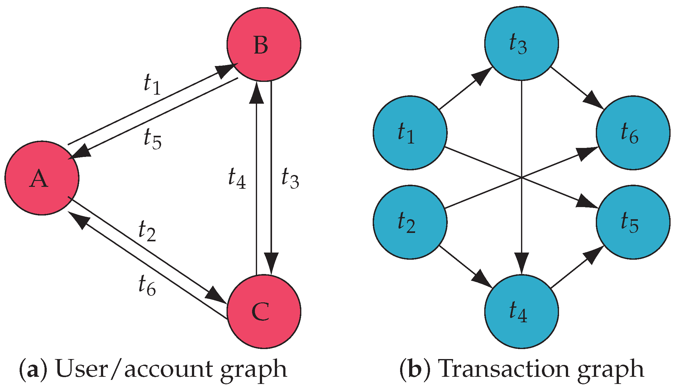
- The blockchain transaction graph lacks closed loops, which causes the GCN to fail to learn where the money is going, reducing the accuracy. For example, in Figure 1a, the user/account graph of financial transactions has loops due to frequent transactions between accounts, so the sources and destinations of funds can be embedded using a directed GCN. Nevertheless, if we convert the graph to a transaction graph of blockchain, shown in Figure 1b, because of the chronology of transactions, it cannot have closed loops, which prevents the GCN from aggregating the destination information in the directed transaction graph.
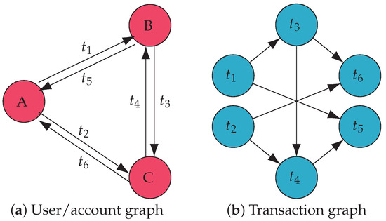 Figure 1. Money laundering through financial and blockchain transactions.
 - The GCNs suffer from an over-smoothing problem, since transaction graphs have vast numbers of nodes, further reducing the accuracy of the detection results. When the user/account graph is converted to the transaction graph, the original transaction edges become nodes. For example, , the first transaction, transfers funds to account B in Figure 1a. Subsequently, account B initiates two transactions, and . Therefore, in Figure 1b, points to both and . We observe that the transaction graph often has more nodes than the user/account graph. This is because, due to frequent transactions between accounts, the number of nodes in the account graph remains constant while the number of nodes in the transaction graph increases. For example, Figure 1a has only three nodes, but when converted to Figure 1a, there are six. In the GCNs, node A only needs to aggregate the information of two nodes (B and C), and node needs to aggregate the data of four nodes (, , , and ). Moreover, if the nodes in Figure 1a make more complex transactions, the nodes in Figure 1b are more numerous and require deeper GCNs to capture the complete information. These will speed up the over-smoothing.
To solve the above issues, we propose a novel graph deep learning method named the Long-Term Bi-Graph Layer Attention Convolutional Network, denoted as LB-GLAT. Concisely, we constructed a bi-graph model. The forward graph aggregates the source information of the blockchain transactions, while the reverse graph aggregates the destination information. Meanwhile, we designed a long-term layer attention mechanism to eliminate the effect of over-smoothing caused by extensive blockchain transaction nodes. The three main contributions of this study are as follows:
- We considered the differences between financial and blockchain transactions and addressed the implications of these differences.
- To solve the problem of being unable to detect the whereabouts of funds due to the chronological order of the transaction graph, we proposed the use of a bi-graph, including a transaction graph and a reverse transaction graph, to detect the source and destination of money laundering activities using blockchain.
- We designed a long-term layer attention mechanism that can combine the characteristics of money laundering at each stage and alleviate the over-smoothing problem.
This paper is structured as follows: Section 2 describes the related work on anti-money laundering in blockchain; Section 3 provides an overview of the LB-GLAT model and describes the model details; Section 4 describes the training data characteristics and the details of the training process; Section 5 illustrates our experimental setup and corresponding results; and Section 6 summarizes this paper.
2. Related Work
This section reviews the existing literature related to our work. We classify blockchain anti-money laundering methods into machine-learning-based methods and deep-learning-based methods. Additionally, we analyze their respective characteristics and highlight the differences between previous studies and our research.
2.1. Machine-Learning-Based Methods
The traditional methods for detecting blockchain money laundering are the classification and clustering machine learning models, using the local information of blockchain transaction data or adding hand-crafted structural features, such as the node degree, eigenvector centrality, and clustering coefficient. Standard algorithms include Logistic Regression [14], Decision Tree [15], Support Vector Machine [16], and K-means Clustering [17]. In 2017, Pham et al. [10] adopted the modified K-means Clustering method to detect suspicious behavior on two graphs generated by Bitcoin transactions, one graph with users as nodes and the other with transactions as nodes. The same year, Pham et al. [18] compared three unsupervised machine learning methods on these graphs, including K-means Clustering, Mahalanobis Distance, and a Support Vector Machine. However, due to the small size of the dataset without GPU support, in 2019, Yang et al. [11] used an unsupervised Gaussian mixture model to cluster users and detect abnormal transactions between suspicious users.
To solve the problem of label scarcity with supervised algorithms, Lorenz et al. [19] proposed an active learning solution in 2020, which was able to match the performance of a fully supervised baseline using only 5% of the labels. Li et al. [20] proposed a model that integrated LSTM into an automatic encoder and used a time window to generate time features. The result showed that the generated features were helpful for the identification of illegal addresses. Alarab et al. [21] proposed an ensemble learning method, which used a given combination of supervised learning models, and found that it was superior to the classical learning model used in the original paper. In 2021, Vassallo et al. [22] proposed an Adaptive Stacked Extreme Gradient-Boosting method, which successfully reduced the impact of concept drift and further improved recall at a transaction level. Other papers have also compared the performance of several supervised or unsupervised machine learning algorithms [9,23]. For example, in 2022, Pettersson et al. [9] compared four supervised learning algorithms and calculated the fitting and applicability of each algorithm. The results showed that the effect of random forest was better than that of other algorithms.
The characteristics of a simple structure, short training time, and low data dependence mean that machine learning algorithms are still used for anti-money laundering. However, they have some severe drawbacks. Machine learning algorithms have limited parameters and are sensitive to data quality, especially noise and abnormal data. Furthermore, they rely on manually selected features and function design, resulting in a weak generalization ability. In addition, even if hand-crafted structural features are used, it is difficult for algorithms to find certain complex money laundering activities that contain rich money laundering features in a graph structure. Therefore, we used deep learning algorithms to implement anti-money laundering in order to avoid these drawbacks.
2.2. Deep-Learning-Based Methods
Money laundering algorithms based on deep learning are applied to graphs, and they can effectively use the graph structure to identify money laundering behavior. For example, Hu et al. [24] found that the main differences between money laundering and conventional transactions lie in their output values and neighborhood information, and they evaluated a set of classifiers based on four types of graph features, among which the node2vec-based classifier was superior. Poursafaei et al. [25] proposed an effective graph-based solution called SIGTRAN, which could detect illegal nodes on blockchain networks and be applied to records extracted from different networks. Experiments were conducted using data from the literature on Bitcoin and Ethereum, respectively, and the proposed model outperformed the more complex, platform-dependent models.
With the publication of the graph convolution network (GCN) by Kipf et al. [26], more and more researchers began using graph neural networks to study anti-money laundering on blockchain. There are many types of GCNs and their variants, and since the transaction network is a directed graph, it is more suitable to adopt spatial-domain GCN algorithms [27]. The GCNs mentioned later in this paper are all spatial-domain GCNs. The simplest spatial-domain GCN replaces the symmetric normalized Laplacian matrix with random walk normalization when aggregating information. Other common examples are the graph attention network (GAT) [28] and graph sample and aggregate (GraphSAGE) [29]. Among these, GAT adds a self-attention mechanism when the network aggregates neighbor information, while GraphSAGE samples neighbor nodes before applying the aggregation function.
There has been much research based on graph neural networks. For example, Weber et al. [12] from IBM LABS provided the Ellipse dataset in 2019, the largest labeled transaction dataset publicly available in any cryptocurrency, and used it to train a GCN model. Alarab et al. [13] tried to explore the convolution of graphs in a novel way using the existing graph convolution network interwoven with linear layers for modeling. Han et al. [1] trained a multi-graph convolutional neural network (GNN-FiLM) with a blockchain transaction graph and solved the data imbalance problem using K-rate sampling and feature similarity methods. Li et al. [6] put forward the weighted GraphSAGE method and added a priority sampling layer, which significantly improved the effect and proved the necessity of priority sampling.
However, these studies did not consider the differences between blockchain transactions and financial transactions, including the absence of transaction closed loops due to chronological order and the accelerated over-smoothing caused by excessive nodes and the deepening of layers. Therefore, we propose the LB-GLAT model based on a spatial-domain GCN, which uses a bi-graph and a long-term layer attention mechanism to solve these problems. It is an inductive algorithm that can predict other nodes that are not on the graph. Moreover, in experiments, we compared some of the algorithms in the abovementioned papers with our algorithm to prove the feasibility of LB-GLAT.
3. Model Architecture
This section introduces our proposed model, the Long-Term Bi-Graph Layer Attention Convolutional Network (LB-GLAT). We first analyze the overall architecture of the model. Next, we provide details about the essential modules of the model.
3.1. Overview
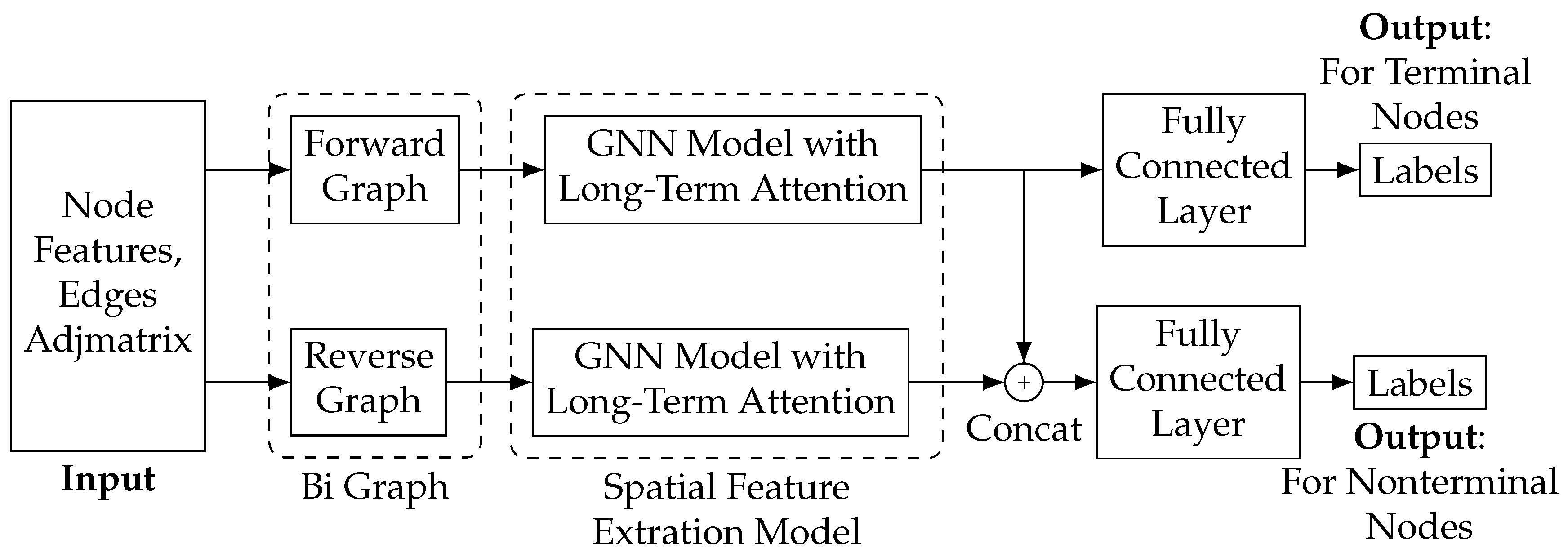
We designed LB-GLAT considering blockchain transaction characteristics to effectively capture the topological structure and attribute characteristics of money laundering on a blockchain transaction graph. The model architecture is shown in Figure 2. The input data are transaction node features, such as the transaction amount and node adjacency matrix constructed by flow edges between transactions. The model’s output is the classification result, which evaluates the transaction status. The essential module of the model is visualized as follows:

Figure 2.
Overview of LB-GLAT.
- Bi-Graph: To address the limitation of the GCN in capturing the money laundering structure due to the absence of loops in the blockchain transaction graph, we adopted a bi-graph module. This module creates a reverse graph from the forward graph, allowing the model to learn the characteristics of both the source and destination of transaction funds.
- Spatial feature extraction: To better capture the money laundering structure, we designed a spatial feature extraction module that convolves the forward and reverse transaction graphs multiple times. Additionally, we incorporated a long-term layer attention mechanism to mitigate the over-smoothing problem of the GCN. This module independently learns money laundering information from the node features aggregated by the GCN each time, and the result is input into the classification head.
- Classification head: Since a transaction graph can consist of transactions over a certain period, some nodes may have a zero in-degree on one or both graphs. To address this issue, we created two classification heads. Depending on whether a node’s in-degree is zero on both graphs, the node vectors obtained from the spatial feature extraction module are divided into two categories and input into the corresponding classification head to obtain the node classification label.
During training, LB-GALT processes transaction graphs from a specific period in batches. For each set, two graphs are constructed: a forward graph and a reverse graph, which are used to learn the destination information of transactions. The spatial feature extraction module, a GCN model equipped with long-term layer attention, then learns the money laundering characteristics hidden in these two graphs. This module generates two node vectors containing the source and destination of money laundering information, respectively. Finally, nodes are grouped according to the in-degree in both the forward and reverse graphs, and the node vectors are input into different classification heads. The inference process of the model follows the same approach as the training process. In this paper, the transaction graph is not fully connected, and the type of prediction task is inductive. In the following sections, we provide a detailed introduction to each module.
3.2. Spatial Feature Extraction Module
In this section, we mainly introduce the spatial feature extraction module, designed to extract features from the transaction nodes in the transaction graphs. Note that we initialized two separate spatial feature extraction modules with different parameters for the forward graph and the reverse graph in the bi-graph. Therefore, this section focuses on the spatial feature extraction module itself without distinguishing between the forward graph and the reverse graph.
The spatial feature extraction module was used to reduce the problem of accuracy reduction caused by over-smoothing [30,31,32] and better extract the money laundering characteristics in the transaction graph. It contained a spatial-domain GCN network and a long-term layer. The long-term layer could pay attention to the money laundering information extracted by the GCN each time and aggregate it into node vectors.
3.2.1. Spatial-Domain GCN
The spatial graph convolutional neural network proposed by Bruna et al. [33] in 2013 has garnered significant attention in recent years. The spectral-domain GCN proposed by Kipf et al. [26] in 2017 has certain limitations, such as being a transductive inference learning method that becomes computationally expensive as the number of nodes in the graph increases. To address these limitations, the spatial-domain GCN has become a popular alternative, as it is inductive and can be applied to various graphs. In this work, we focused on the widely used random walk normalized adjacency matrix to convolve nodes in the transaction graph.
The transaction graph differs from the user/account graph in financial transactions. It consists of transactions as nodes and the flows of transaction funds as edges. The graph has m nodes, defined as , and numerous directed edges , which indicate that node points to node . Using Equation (1), we can calculate the adjacency matrix and degree matrix of the nodes, where represents the in-degree of node . Therefore, the degree matrix D is essentially a diagonal in-degree matrix of the nodes.
The node vector comprises n primitive transaction features, such as the number of inputs/outputs and the average amount received/spent. The node feature vectors and adjacency matrix A composed of m nodes as a batch are fed into a GCN and convolved L times. Each convolution is recorded as one layer, that is, we have a L-layer GCN. The node vectors obtained by the convolution of the l-th layer of the GCN are denoted as , where is the node feature dimension of the l-th layer. When , is the input data X, and the feature dimension is n.
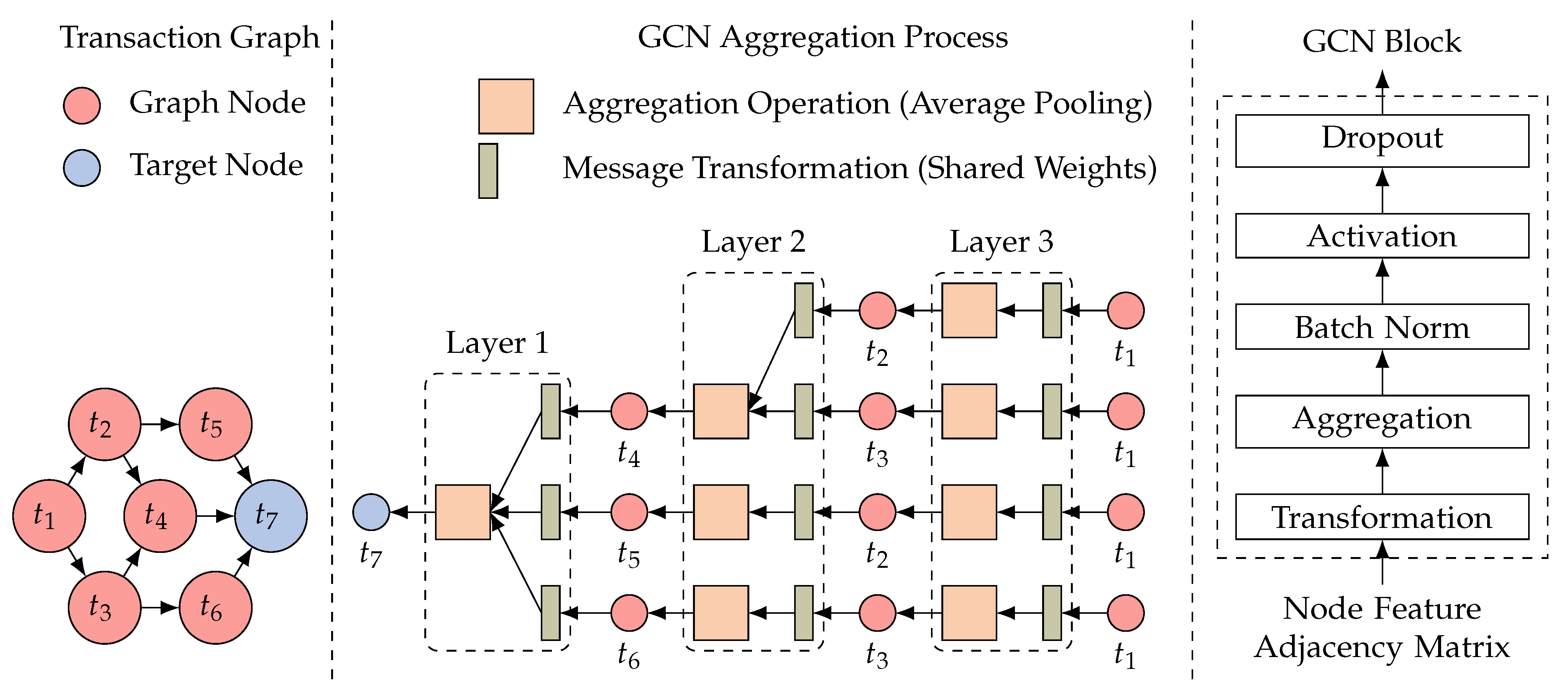
The convolution process for each layer of a spatial-domain GCN for a directed graph consists of two main steps: message transformation and aggregation. Let us consider the l-th layer as an example to describe the process. Firstly, all -th layer node vectors are multiplied by a learnable shared parameter , which is equivalent to transforming the node messages. This transformation allows the model to capture different features and patterns in the graph data. Then, the information of the node and its neighbors pointing to the node is applied to an average aggregation function to obtain the node vectors after the convolution of the GCN at the l-th layer. The aggregation function is typically an average pooling function, combining information from neighboring nodes to create a more robust representation of the current node. The convolution process can be represented by Equation (2), where is the activation function, which is typically set to , and is the random walk normalized adjacency matrix of A. To aggregate the node information itself, adjacency matrix A is added to identity matrix I to obtain , and the in-degree matrix of is calculated. Then, is equivalent to , averaged according to the node in-degree. Finally, is multiplied by the transformed vector to calculate . Using the random walk normalized adjacency matrix allows the GCN to capture the structural information of the graph more effectively. By averaging the adjacency matrix according to the node in-degree, the model can selectively focus on the most important nodes in the graph, enhancing the representation of the node features. Overall, the convolution process in a spatial-domain GCN for a directed graph effectively captures both local and global information in the graph data, allowing the model to learn powerful representations for downstream tasks.
Figure 3 illustrates the spatial-domain GCN convolution process for target node with three layers. In the first layer (), the features of are derived from its neighboring nodes, specifically , , and . In the second layer (), the features of are enriched with information from its neighbors, including and , resulting in receiving features from and . Similarly, in the third layer (), the structural information of propagates to the feature of through the same mechanism. The convolution process is performed in each layer using the GCN blocks depicted in the figure. To improve the generalization ability of the model, each GCN block applies a Batchnorm process before the activation function and a dropout layer after . Thus, in Equation (2) is rewritten as Equation (3).

Figure 3.
The convolution process of a GCN: message and aggregation.
3.2.2. Long-Term Layer Attention
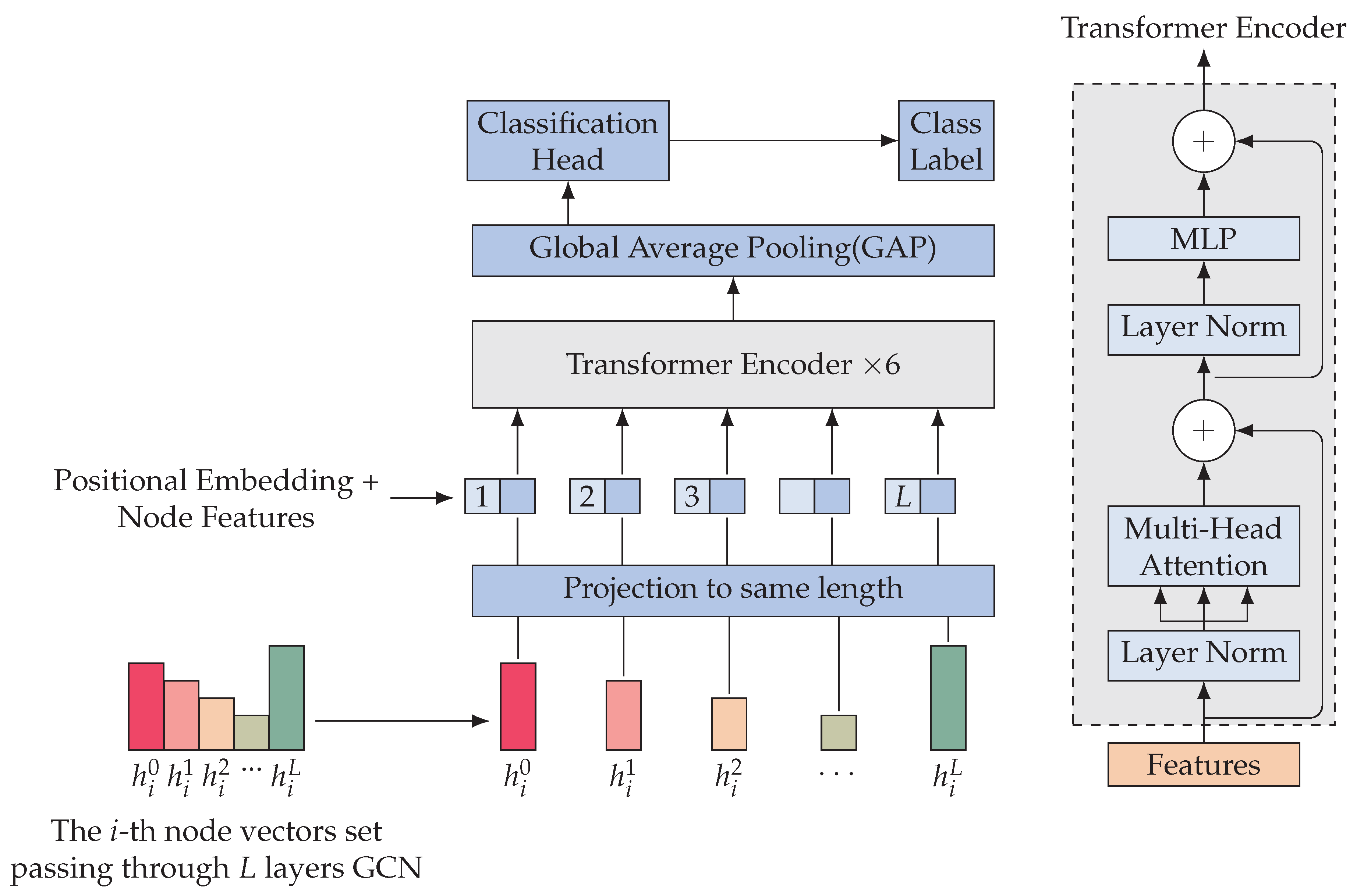
The long-term layer attention mechanism utilizes the transformer encoder and is inspired by the vision transformer [34] model architecture. After L layers of GCN convolution, we obtain a set of node vectors of length . In our model, the number of layers L is set to four, as depicted in Figure 4. The target node is set to , and the node feature set of is represented as . Taking Figure 4 as an example, we illustrate the mechanism of long-term layer attention.
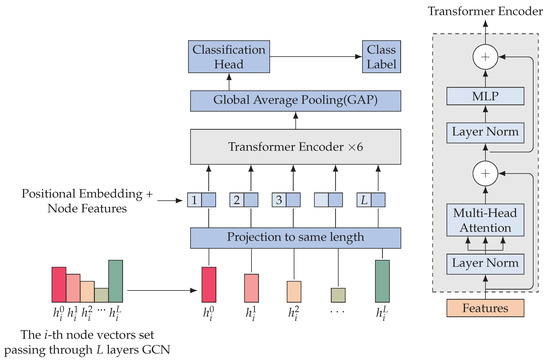
Figure 4.
An overview of long-term layer attention.
In the GCN, each convolutional layer can produce a different feature dimension for the node features. Specifically, the length of may vary depending on l. To address this issue, we employed a learnable projection layer that projects the node feature produced by each GCN layer to a fixed length d. For simplicity, indicates the node features after the projection layer in the following description.
In the transformer encoder, each element in contains L-hop neighbor information, and the order of elements matters. To preserve positional information, learnable 1D position embeddings are added to the projected node features. The resulting vectors are then fed into the transformer encoder. Considering the i-th node as an example, the encoder input can be represented by Equation (4). L is the number of layers in the spatial-domain GCN, and d is the dimension of the node embeddings after the projection layer. The input vector consists of the projected node vector and the learnable position embeddings . The superscript 0 indicates that this is the input to the first layer of the transformer encoder.
The transformer encoder consists of alternating layers of multi-headed self-attention (MSA) and multi-layer perception (MLP). Before both MSA and MLP, a Layernorm (LN) process is applied, and afterwards, there is a residual connection of the previous MSA or MLP. The process can be described by Equation (5).
We used the standard self-attention mechanism for MSA. We set , , and to be 2D matrices with dimensions . In the k-th alternating layer, the input sequence is multiplied by a trainable parameter , and the result is divided into , , and (Equation (6)). We calculate the pairwise similarity of and between two elements in the sequence, denoted as the attention weight (Equation (7)). Then, we compute the weighted sum of value matrix with respect to (Equation (8)).
The multi-headed self-attention (MSA) module runs s self-attention processes in parallel and projects their concatenated outputs (Equation (9)).
We applied a global average pooling (GAP) operation to the vectors obtained after the encoder. Equation (10) computes the result vector of node . All node result vectors are then taken as input to the classification head.
3.3. Bi-Graph
In real-life scenarios, identifying money laundering in transactions relies on observing specific patterns exhibited by the source and destination of the funds involved. When employing deep learning techniques for detecting blockchain-related money laundering, a model should acquire knowledge of the distinctive characteristics and patterns associated with the source and destination of transaction funds. However, due to the inherent limitations of transaction graphs in the blockchain, which prevent the formation of loops, directed transaction graphs are unable to consolidate the destination information of the funds effectively.
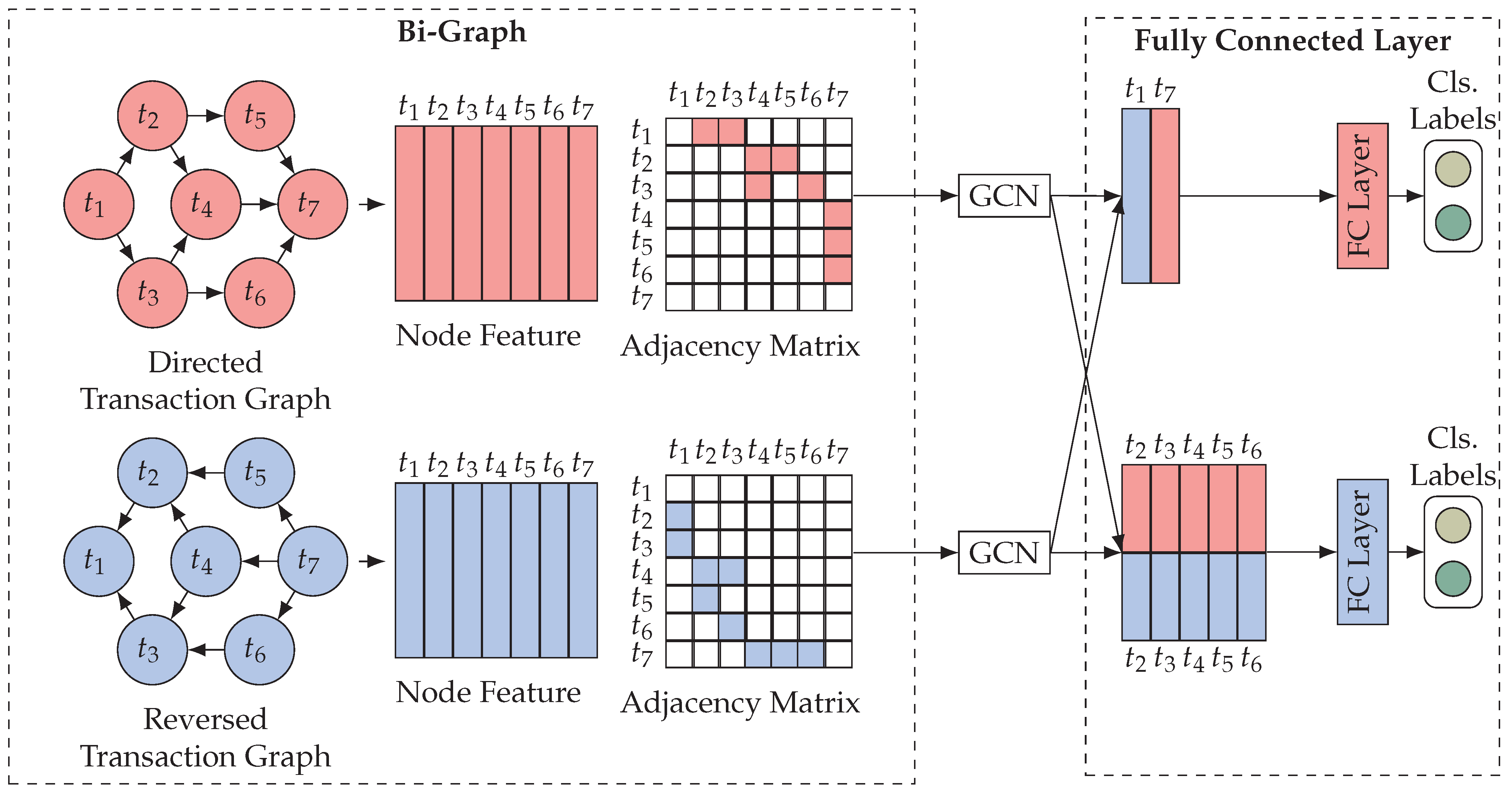
To address the issue, we employed a bi-graph strategy that utilizes a forward graph and a reverse graph. It is worth noting that this approach is not novel, as many researchers have already embraced it [35]. Illustrated in Figure 5, we introduce the concept of a forward graph and a reverse graph , where both graphs share the same set of nodes . Furthermore, the presence of an edge implies the existence of a corresponding edge , denoted as . In other words, the adjacency matrix of , denoted as , satisfies , where represents the adjacency matrix of .
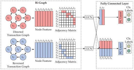
Figure 5.
Bi-graph model.
To analyze the transaction graph, we constructed the forward graph and the reverse graph . The node features X along with the adjacency matrices and of and are separately inputted into distinct spatial feature extraction modules. Consequently, we obtained the node embeddings and for each node within and , respectively.
3.4. Classification Head
The directed GCN is limited in aggregating neighbor information directed towards the node. Consequently, if a node has no in-degree in either the forward or reverse graph, the convolution operation of the GCN loses its significance. To address this, we introduced two classification heads within the architecture, enabling the fully connected network to learn distinct money laundering information from different nodes. Each classification head consists of two hidden layers with the activation function , followed by an output layer with the activation function . Before the activation, each hidden layer incorporates , while a dropout layer is applied after the activation. It is important to note that the input vectors differ for each classification head, allowing each head to perform a unique role.
To be more precise, the nodes are classified based on their in-degree in both the forward graph and the reverse graph , resulting in two distinct node sets. Set represents nodes that possess in-degree in both the forward and reverse graphs. On the other hand, set denotes the absolute complement of within the complete node set , indicating nodes that do not meet the criteria set by . For instance, in Figure 5, and .
The nodes in set can also be divided into two subsets according to their in-degree status in the two graphs. Subset indicates that the node has only an in-degree in forward graph , or discrete points. Discrete points are special, and we place them in . Conversely, subset indicates that the node has only an in-degree in reverse graph . For example, in Figure 5, and .
After the spatial feature extraction module, we obtained the convolved vectors for the forward graph and for the reverse graph of all nodes. Let us consider node as an example. If , we concatenate vectors and , using the resulting vector as the input for classification head 1 (Equation (11)). This allows us to learn the source and destination information of transaction funds. On the other hand, if , we take either vector or as the input for classification head 2 (Equation (12)), enabling us to learn the source or destination information of transaction funds. This approach is justified by the inherent symmetry often found in money laundering structures, where illicit funds disperse from one node and converge towards another. By utilizing two classification heads and having sufficient data, it becomes possible to learn the source and destination information separately.
After all nodes pass the classification heads, the probability of illicit and licit is obtained. The training loss is then calculated using the cross-entropy loss function (Equation (13)), and the model parameters are updated by back-propagation.
4. Implementation
In this section, we describe the dataset (Section 4.1) and the parameter settings for the model training process (Section 4.2).
4.1. Dataset
The dataset used to evaluate our model was the Elliptic dataset, published by the MIT-IBM Watson AI Laboratory [12]. This dataset is the most extensive publicly available labeled transaction dataset across any cryptocurrency [12]. Within the Elliptic dataset, each Bitcoin transaction represents a genuine entity encompassing licit transactions (such as exchanges, wallet providers, miners, and legitimate services) and illicit transactions (such as terrorist organizations, ransomware, and Ponzi schemes).
The dataset transforms the raw Bitcoin transaction data into the structure of a transaction graph. The nodes are the transactions in the Bitcoin blockchain (203,769 transactions), and the edges are the flows between transactions (234,355 flows). Of these nodes, two percent (4545) are labeled as illicit. Twenty-one percent (42,019) are labeled as licit. The remaining nodes are not labeled with any category, so they were not used in our model evaluation process.
Each node has 166 features. The first 94 features represent the local information of the transaction, including the time step, number of inputs/outputs, transaction fee, output volume, and other aggregated figures. The remaining 72 features represent aggregate information, that is, the aggregation features of the same information of the neighboring nodes, including the maximum, minimum, standard deviation, and correlation coefficients. Each node has a timestamp that divides all nodes into 49 time steps with an interval of about two weeks. In different time steps, there is no edge connection. Namely, the 49 graphs are independent of each other.
4.2. Training
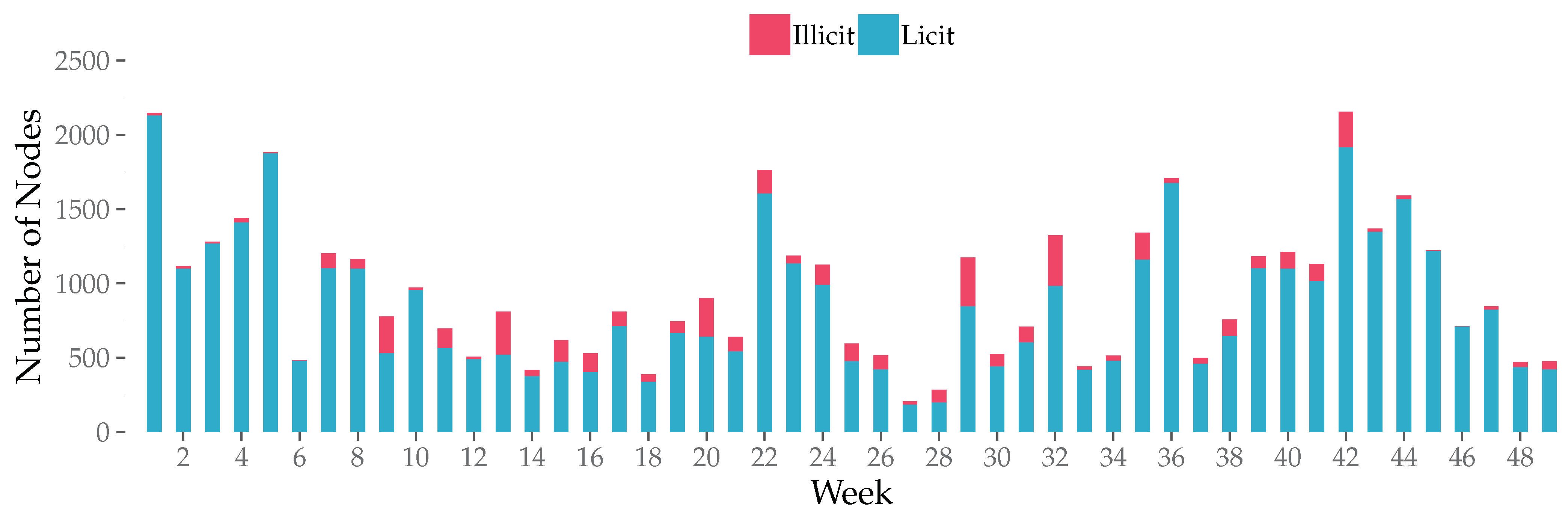
We adjusted the hyper-parameters of the LB-GLAT model empirically. Table 1 shows the parameters. For the Elliptic dataset, we removed the timestamp feature and used only the remaining 165 node features. The data for each time step were divided into training (80%), validation (10%), and test (10%) sets. However, the positive and negative samples were severely unbalanced in each time step, as shown in Figure 6. To balance the samples, we adopted the under-sampling approach so that the ratio of illicit to licit samples was 1 to 5. The nodes for each time step were fed into the model as a batch, and the unused data were masked. The training super-parameters are shown in Table 1.

Table 1.
The parameter settings of the LB-GLAT model.
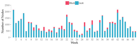
Figure 6.
Number of licit and illicit nodes per time step.
We trained the model for 200 epochs using the optimizer with a learning rate of 0.01 and a weight decay of . The learning rate decayed with the increase in epochs, and the decay coefficient was , where the decay rate was set to 1. During the training process, we adopted the early stop strategy, took the model parameters with the least loss in the validation set, and tested them using the test set.
In our model, we used four layers for the GCN in the spatial feature extraction modules of both the forward graph and reverse graph. The node embedding size of each GCN layer was set to 32, which was our tuned parameter. The initial node features and the resulting vectors of each GCN layer were applied to a projection layer with a dimension size of 32, transforming them to the latent vector size in the transformer encoder. The vectors passed through a dropout layer after the projection layer to prevent over-fitting and were fed into the encoder. In the transformer, to learn the money laundering information hidden within the vector of each GCN layer, we used four attention heads, each with a size of 8, and the MLP hidden layer size was set to 64. The two hidden layer sizes of the classification head were 64 and 32, respectively. All dropout values in the model were 0.5.
4.3. Complexity Analysis
In LB-GLAT, the bias was set to true. However, for the sake of complexity analysis, we ignored the bias. Additionally, we also disregarded operations like activation functions that did not affect the order of complexity.
Firstly, the computational complexity of the l-th layer of the GCN was , so the computational complexity of the GCN with L layers was , where represents the node feature dimension of the l-th layer. Then, the node feature produced by each GCN layer was projected to dimension d, which had a computational complexity of . Next, these vectors were fed into the transformer encoder, which consisted of K alternating layers of MSA and MLP. The computational complexity of the transformer encoder was , where represents the hidden layer size of MLP in the transformer. Because of the bi-graph module, the computational complexity of the two spatial feature extraction modules was . Subsequently, all node vectors were fed into the classification heads. The computational complexity of the two classification heads was , where each classification head had two hidden layers, and represents the i-th layer size of the j-th classification head.
Therefore, the computational complexity during training was , where E, U, and represent the number of training epochs, the batch size, and the sub-batch size in the j-th classification head (), respectively. The computational complexity during inference was .
5. Experiment
In this section, we evaluate LB-GLAT through several experiments: a correctness experiment to evaluate whether the model converged during the training process, ablation experiments to evaluate the effectiveness of various components in LB-GLAT, and comparison experiments with several state-of-the-art methods. Section 5.1 describes the experimental setup. Section 5.2 lists and analyzes the experimental results.
5.1. Experimental Setup
We conducted experiments using the PyTorch deep learning framework, Pyg graph neural network framework, and Sklearn machine learning toolkit.
(1) Training process
We trained LB-GLAT on the Elliptic dataset for 200 epochs and observed the loss curve trend of the training set and validation set during the training process. If both loss curves showed a similar downward trend, LB-GLAT converged, and the model establishment process was correct. The training details can be found in Section 4.2.
(2) Ablation experiments
To evaluate the effectiveness of the components in LB-GLAT, we performed a series of ablation experiments. Firstly, we created a model called “No-BG”, which excluded the bi-graph structure from LB-GLAT, allowing us to examine the importance of incorporating the bi-graph. Additionally, the original model utilized long-term layer attention (LTLA) in the spatial feature extraction module. Therefore, we investigated the scenario in which LTLA was removed from the model, resulting in a model named “No-LTLA”. Furthermore, our model employed a GCN as the convolutional layer for extracting money laundering information from the transaction graph. To assess the effectiveness of the GCN, we replaced the GCN with the other two commonly used spatial graph convolutional networks:
- GAT—GAT [28] is a GCN network combining masked self-attention layers. The model allows different weights to be implicitly assigned to different nodes in the neighborhood and is suitable for induction and transformation problems.
- GraphSAGE—GraphSAGE [29] is a popular graph neural network for large graphs. The model learns a function to generate embeddings by sampling and aggregating features from a node’s local neighborhood.
The replacement models were named GAT-No-GCN and GraphSAGE-No-GCN, respectively. These models were evaluated by five indicators commonly utilized in classification problems, including accuracy, precision, recall, F1−score, and area under the curve (AUC) [36], as shown in Equation (14). Here, P and N represent the number of positive and negative samples, respectively; (true positive), (false positive), (true negative), and (false negative) represent the number of positive samples predicted as positive classes, negative samples predicted as positive classes, negative samples predicted as negative classes, and negative samples predicted as positive classes, respectively; and and , used in calculating the AUC, stand for the probability that a sample is predicted to be positive or negative, respectively. Precision, recall, and F1−score were all calculated using illegal samples in the experiments. For ease of description, we refer to the above five evaluation indicators of model m in the experiments as , , , , and , respectively.
(3) Comparison experiments
We employed the following methods and state-of-the-art models widely used in blockchain anti-money laundering as baselines to highlight the effectiveness of our proposed model:
- LR: Logistic Regression [14] is a statistical method commonly used for binary classification. We applied the L2 normalization set inverse of regularization strength . We set the tolerance for stopping criteria to and the max iterations to 200 and used liblinear [37] as the solver for the optimization algorithm.
- DT: Decision Tree Classifier [15] is a machine learning method used to build predictive models from data. The model divides the data space recursively, fits a simple prediction model into each partition, and measures the error using misclassification costs. We set the minimum leaf sample to five to prevent over-fitting and the gini coefficient as the impurity criterion.
- SVM: Support Vector Machine [16] is a machine learning method for classification problems. It maps the input vector nonlinearly to a very high-dimensional feature space. A decision surface for classification is constructed in the feature space. We applied the Gaussian kernel as a kernel function in SVM.
- GCN: The GCN used in the experiment was the same as in our paper. We applied a four-layer spatial-domain GCN with a node embedding size of 32 for each layer and then passed through an MLP module of two hidden layers with sizes 64 and 32. We refer to this model as GCN+MLP in later experiments.
- GNN-FiLM: GNN-FiLM was used by Han et al. [1] for the anomaly detection of blockchain. They used k-rate sampling for the data and labeled unknown transaction nodes by feature similarity to reduce the imbalance between positive and negative samples.
- Weighted GraphSAGE: Weighted GraphSAGE [6] is an improved GraphSAGE method based on weighted sampling neighborhood nodes. This model is trained to learn more efficient aggregate input features in the local neighborhood of nodes in order to find and analyze the implied interrelationships between blockchain transaction features.
- GCN assisted by linear layers: This is a novel approach proposed by Alarab et al. [13] for modeling using the existing graph convolutional network intertwined with linear layers. The node embeddings obtained from the convolutional layer of the graph are connected with a single hidden layer obtained from the linear transformation of the node feature matrix, followed by a multi-layer perception layer. In the later experiments, we refer to this model as GCN-linear for short.
Among these methods, GNN-FiLM, weighted GraphSAGE, and GCN-linear are models designed for blockchain anti-money laundering, and their original papers also included experiments on the Elliptic dataset. We also used two baselines mentioned in the ablation experiment, GAT and GraphSAGE, for comparison with LB-GLAT. These were set to the same parameters as GCN+MLP and named GAT+MLP and GraphSAGE+MLP. These models were also evaluated using the indicators in Equation (14).
5.2. Experiment Results
We performed experiments according to the set parameters and describe the results of the experiments below.
5.2.1. Training Process
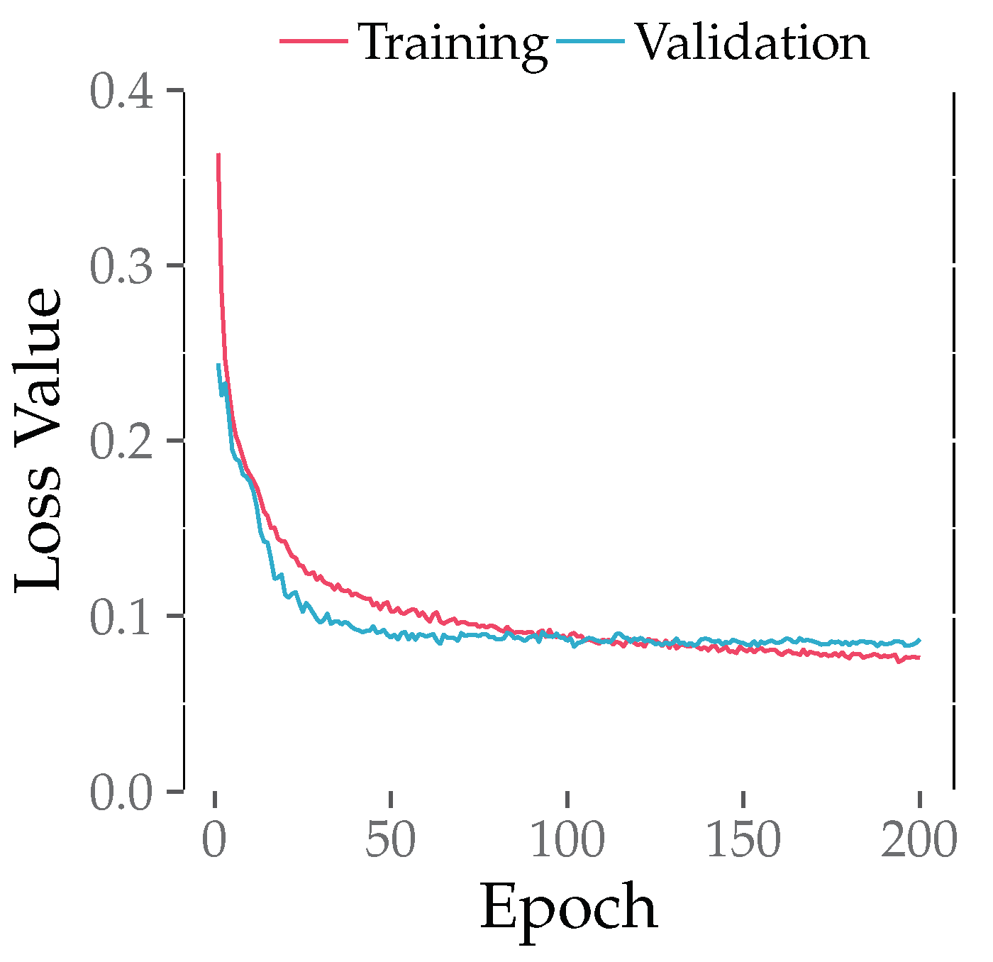
We conducted a training process for LB-GLAT and observed the loss of both the training set and validation set. The results are shown in Figure 7. The training loss represents the mean loss value after training for each batch, while the validation loss indicates the loss after training for each epoch. Notably, during the early stage, the validation loss was smaller than the training loss. In Figure 7, the training loss decreased as the number of epochs increased, indicating the convergence and correctness of our model. Similarly, the validation loss decreased initially with the increase in epoch count and later stabilized. Continuing training beyond this point only yielded limited improvement in model performance. Therefore, we set the epoch count to 200 and tested the model on the test set when the validation loss was at its lowest point.
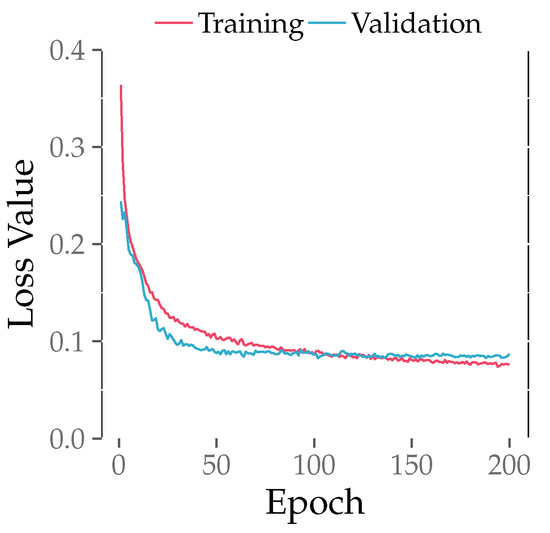
Figure 7.
The loss of the training set and validation set during LB-GLAT training.
5.2.2. Ablation Experiments
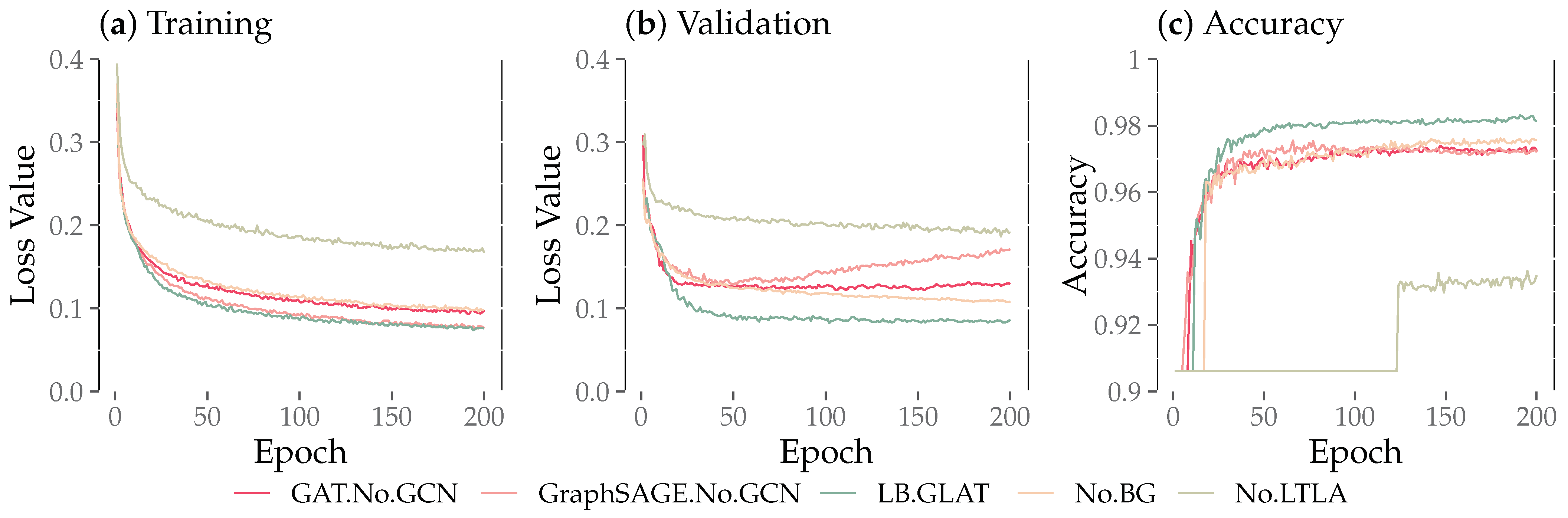
Figure 8a shows the comparative results of the training losses for the ablation experiment. All training loss curves declined rapidly in the early stage and flattened out in the later stage. Among them, the training loss curves of LB-GLAT and GraphSAGE decreased the fastest, but in the validation loss comparison of Figure 8b, GraphSAGE quickly presented over-fitting, while the LB-GLAT validation loss curves decreased until flattening, to a lesser extent than GraphSAGE, presenting the best results in these ablation experiments. Moreover, as shown in Figure 8c, LB-GLAT had the highest accuracy, reaching about 0.98. We used an early stop strategy and selected the model with minimal validation loss to test the five evaluation indicators on the test set. The results are shown in Table 2. We underlined the highest value of each evaluation indicator. LB-GLAT achieved the best experimental results on all indicators, with reaching 0.9776, reaching 0.9317, reaching 0.8494, reaching 0.8887, and reaching 0.9806.
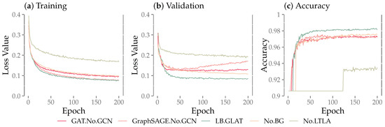
Figure 8.
The comparison of loss and accuracy between LB-GLAT and the four other ablation experiments.
Table 2.
The results of the five evaluation indicators for LB-GLAT and the four other ablation experiments using the test set.
From the results of the ablation experiments, we obtained the following three findings regarding the components of LB-GLAT, showing that each of our components had a very important role. The first finding was that the LTLA component achieved the best results and could effectively learn the money laundering characteristics of blockchain transactions hidden within each convolutional layer. Compared with the GCN+MLP model in Table 3, the No-BG model, which only applied the LTLA component on the basis of GCN+MLP, presented a very high increase in all indicators, especially , which increased by 23%. This shows that LB-GLAT could effectively learn the hidden money laundering information when the convolutional layer vectors implemented the self-attention mechanism.
Table 3.
The results of the five evaluation indicators for LB-GLAT and the other methods using the test set.
The second finding was that the BG component, while not as effective as LTLA, played an important role. For the No-LTLA model with only BG, compared to GCN+MLP, only the precision and AUC indicators increased, by less than 6% and 1%, respectively, presenting lower values than the indicators of the No-BG model with only LTLA. However, the indicators of LB-GLAT, which applied the BG and LTLA, were higher than those of the No-BG model, indicating that the BG could capture the source and destination of the transaction funds. LTLA could fully learn the information about the destination of funds contained in the results of each layer convolved on the reverse graph.
The final finding was that the GCN performed better than GAT and GraphSAGE when the BG and LTLA components were applied. GAT assigned weights to different neighbor nodes, and GraphSAGE sampled neighbor nodes. Therefore, the difference between the three convolution methods was that GAT and GraphSAGE did not treat every neighbor node equally, discarding the information of some neighbor nodes. This led to the loss of money laundering characteristics on the Elliptic dataset, so GCN worked better.
5.2.3. Comparison Experiments
Table 3 shows the results of the comparison experiments and underlines the highest values of each evaluation indicator and the results of our model, LB-GLAT. The first three models are machine learning algorithms trained according to the parameters in Section 5.1, of which DT had the best evaluation results. Its and results were the highest among all the algorithms, reaching 0.9779 and 0.8872, respectively. The other models are graph neural network algorithms. Among them, the GAT+MLP model had the worst evaluation results. Since the model does not predict positive labels, and are not reported in the literature, as indicated by “-”, and is 0. The results of GNN-FiLM, weighted GraphSAGE, and GCN-linear were the best results obtained by the authors in their respective papers. We also use “-” to denote evaluation indicators not provided in the literature.
We also obtained three findings from the results of comparison experiments. The first and most obvious finding was that LB-GLAT largely outperformed the state-of-the-art algorithms. Its and values were higher than the results of all comparison algorithms, reaching 0.8887 and 0.9806, respectively. In particular, was 28% higher than that of GNN-FiLM and 17% higher than that of GCN-linear. was also 18% and 12% higher, respectively. Regarding the weighted GraphSAGE model, although and were not much higher, they still presented increases of 5% and 1%, respectively. This showed that our model could learn the hidden money laundering characteristics of blockchain transactions more effectively.
The second finding was that DT worked best in machine learning algorithms, but this may have been an illusion. As we all know, the AUC describes a model’s ability to distinguish between positive and negative classes. The closer its value is to 1, the stronger the differentiation ability is, and the AUC is not affected by sample imbalance, so it was a good indicator for the Elliptic dataset. However, was 4.3% lower than the result for our model, even though all other indicators for DT were high. Thus, if DT were tested on another blockchain money laundering dataset with a large amount of data, the evaluation results may not be favorable.
The last and most important finding was the ability of LTLA to alleviate over-smoothing effectively. In Table 3, several evaluation indicators of GAT+MLP are invalid. The reason is that the GAT+MLP model had the same parameters as LB-GLAT and applied four convolutional layers, which caused the model to be overly smooth, and all samples were judged as negative. The comparison of the first two models in Table 4 also confirms this, and we used the F1−score to judge the model’s ability to distinguish positive samples. Meanwhile, we evaluated LB-GLAT’s ability to alleviate over-smoothing. We compared the model with No-LTLA and found that without LTLA, No-LTLA failed when applying five convolutional layers. We also tested DeeperGCN [38], a popular model that alleviates transition smoothing and applies BG components to DeeperGCN. LB-GLAT was able to train very well with 10 convolutional layers, while DeeperGCN could no longer predict positive samples.
Table 4.
The comparison of the F1−score indicator for models using different numbers of convolutional layers.
6. Conclusions
We proposed an LB-GLAT model that combined a bi-graph and long-term layer attention mechanism based on a spatial-domain GCN to learn the information hidden in the transaction graph of blockchains. The experimental results using the Elliptic dataset demonstrated that the method was more effective than other baselines in extracting money laundering information, and its prediction ability was 27% higher than that of the GCN+MLP model. Therefore, our approach has the power to help governments and blockchain users accurately predict money laundering activities and provide a favorable blockchain transaction environment by analyzing behavioral information contained in blockchain transactions.
Our approach has two important components. Since blockchain transactions have chronological order, no closed loop of transactions is formed. If we used a GNN directly, it would only be able to perceive the source of trading funds and not learn where they went. The bi-graph could fully use the information in a directed graph to explore the source and destination of transaction funds. In addition, a transaction network for money laundering may include multi-hop transactions, so the model needs more convolutional layers to obtain money laundering features, but this accelerates over-smoothing. The long-term layer attention mechanism could alleviate the problem of over-smoothing and autonomously learn the money laundering characteristics contained in each layer, thereby greatly improving the model evaluation results.
This study had certain limitations. There is a dearth of open-source money laundering datasets for blockchain research. Given that the Elliptic dataset currently stands as the largest open-source dataset of illicit Bitcoin activities, almost all of the current UTXO-based blockchain anti-money laundering papers have used the Elliptic dataset, and a few have used undisclosed datasets. Therefore, further research endeavors may explore how to extend the dataset to assess the model’s generalizability across an expanded dataset. Additionally, the long-term layer attention mechanism is not only applicable in blockchain anti-money laundering. It can be applied after any convolutional network to learn multi-hop node information and alleviate over-smoothing. Therefore, it may also play an important role in fields that rely heavily on local network architecture.
Author Contributions
Conceptualization, C.G. and S.Z.; methodology, C.G. and S.Z.; software, P.Z.; validation, S.Z. and M.A.; formal analysis, C.G.; investigation, S.Z.; resources, J.S.; data curation, M.A.; writing—original draft preparation, C.G. and S.Z.; writing—review and editing, C.G. and J.S.; visualization, P.Z.; supervision, C.G.; project administration, J.S.; funding acquisition, C.G. and J.S. All authors have read and agreed to the published version of the manuscript.
Funding
This paper was supported by Fundamental Research Funds for the Central Universities under grant No. N2317005 and the National Natural Science Foundation of China under grant No. 62302086.
Data Availability Statement
The source code can be found at https://github.com/NEUSoftGreenAI/LB-GLAT.git, accessed on 12 September 2023.
Conflicts of Interest
The authors declare no conflict of interest.
References
- Han, H.; Wang, R.; Chen, Y.; Xie, K.; Zhang, K. Research on Abnormal Transaction Detection Method for Blockchain. In Proceedings of the International Conference on Blockchain and Trustworthy Systems; Svetinovic, D., Zhang, Y., Luo, X., Huang, X., Chen, X., Eds.; Springer: Singapore, 2022; pp. 223–236. [Google Scholar]
- Zhou, J.; Hu, C.; Chi, J.; Wu, J.; Shen, M.; Xuan, Q. Behavior-Aware Account de-Anonymization on Ethereum Interaction Graph. IEEE Trans. Inf. Forensics Secur. 2022, 17, 3433–3448. [Google Scholar] [CrossRef]
- Alarab, I.; Prakoonwit, S. Graph-Based LSTM for Anti-Money Laundering: Experimenting Temporal Graph Convolutional Network with Bitcoin Data. Neural Process. Lett. 2023, 55, 689–707. [Google Scholar] [CrossRef]
- Ciphertrace. Spring 2020 Cryptocurrency Crime and Anti-Money Laundering Report; Technical Report; Ciphertrace: Los Gatos, CA, USA, 2020. [Google Scholar]
- Grauer, K.; Jardine, E.; Leosz, E.; Updegrave, H. The 2023 Crypto Crime Report; Technical Report; Chainalysis: New York, NY, USA, 2023. [Google Scholar]
- Li, A.; Wang, Z.; Yu, M.; Chen, D. Blockchain Abnormal Transaction Detection Method Based on Weighted Sampling Neighborhood Nodes. In Proceedings of the 2022 3rd International Conference on Big Data, Artificial Intelligence and Internet of Things Engineering (ICBAIE), Xi’an, China, 15–17 June 2022; pp. 746–752. [Google Scholar]
- FATF. Updated Guidance for a Risk-Based Approach to Virtual Assets and Virtual Asset Service Providers; Technical Report; FATF: Paris, France, 2021. [Google Scholar]
- Hallak, I. Markets in Crypto-Assets (MiCA); Technical Report; European Parliamentary Research Service: Brussels, Belgium, 2022. [Google Scholar]
- Pettersson Ruiz, E.; Angelis, J. Combating Money Laundering with Machine Learning—Applicability of Supervised-Learning Algorithms at Cryptocurrency Exchanges. J. Money Laund. Control 2022, 25, 766–778. [Google Scholar] [CrossRef]
- Pham, T.; Lee, S. Anomaly Detection in the Bitcoin System—A Network Perspective. arXiv 2017, arXiv:1611.03942. [Google Scholar]
- Yang, L.; Dong, X.; Xing, S.; Zheng, J.; Gu, X.; Song, X. An Abnormal Transaction Detection Mechanim on Bitcoin. In Proceedings of the 2019 International Conference on Networking and Network Applications (NaNA), Daegu, Republic of Korea, 10–13 October 2019; pp. 452–457. [Google Scholar]
- Weber, M.; Domeniconi, G.; Chen, J.; Weidele, D.K.I.; Bellei, C.; Robinson, T.; Leiserson, C.E. Anti-Money Laundering in Bitcoin: Experimenting with Graph Convolutional Networks for Financial Forensics. arXiv 2019, arXiv:1908.02591. [Google Scholar]
- Alarab, I.; Prakoonwit, S.; Nacer, M.I. Competence of Graph Convolutional Networks for Anti-Money Laundering in Bitcoin Blockchain. In Proceedings of the 2020 5th International Conference on Machine Learning Technologies, Beijing, China, 19–21 June 2020; pp. 23–27. [Google Scholar]
- Friedman, J.; Hastie, T.; Tibshirani, R. Regularization Paths for Generalized Linear Models via Coordinate Descent. J. Stat. Softw. 2010, 33, 1–22. [Google Scholar] [CrossRef]
- Loh, W.Y. Classification and Regression Trees. WIREs Data Min. Knowl. Discov. 2011, 1, 14–23. [Google Scholar] [CrossRef]
- Cortes, C.; Vapnik, V. Support-Vector Networks. Mach. Learn. 1995, 20, 273–297. [Google Scholar] [CrossRef]
- Banfield, C.F.; Bassill, L.C. Algorithm AS 113: A Transfer for Non-Hierarchical Classification. J. R. Stat. Soc. Ser. 1977, 26, 206–210. [Google Scholar] [CrossRef]
- Pham, T.; Lee, S. Anomaly Detection in Bitcoin Network Using Unsupervised Learning Methods. arXiv 2017, arXiv:1611.03941. [Google Scholar]
- Lorenz, J.; Silva, M.I.; Aparício, D.; Ascensão, J.T.; Bizarro, P. Machine Learning Methods to Detect Money Laundering in the Bitcoin Blockchain in the Presence of Label Scarcity. In Proceedings of the First ACM International Conference on AI in Finance, New York, NY, USA, 15–16 October 2020; pp. 1–8. [Google Scholar]
- Li, Y.; Cai, Y.; Tian, H.; Xue, G.; Zheng, Z. Identifying Illicit Addresses in Bitcoin Network; Springer: Singapore, 2020; Volume 1267, pp. 99–111. [Google Scholar]
- Alarab, I.; Prakoonwit, S.; Nacer, M.I. Comparative Analysis Using Supervised Learning Methods for Anti-Money Laundering in Bitcoin. In Proceedings of the 2020 5th International Conference on Machine Learning Technologies, Beijing China, 19–21 June 2020; pp. 11–17. [Google Scholar]
- Vassallo, D.; Vella, V.; Ellul, J. Application of Gradient Boosting Algorithms for Anti-Money Laundering in Cryptocurrencies. SN Comput. Sci. 2021, 2, 143. [Google Scholar] [CrossRef]
- Stefánsson, H.P.; Grímsson, H.S.; Þórðarson, J.K.; Oskarsdottir, M. Detecting Potential Money Laundering Addresses in the Bitcoin Blockchain Using Unsupervised Machine Learning. In Proceedings of the Hawaii International Conference on System Sciences, Maui, HI, USA, 4–7 January 2022. [Google Scholar]
- Hu, Y.; Seneviratne, S.; Thilakarathna, K.; Fukuda, K.; Seneviratne, A. Characterizing and Detecting Money Laundering Activities on the Bitcoin Network. arXiv 2019, arXiv:1912.12060. [Google Scholar]
- Poursafaei, F.; Rabbany, R.; Zilic, Z. SigTran: Signature Vectors for Detecting Illicit Activities in Blockchain Transaction Networks. In Advances in Knowledge Discovery and Data Mining; Karlapalem, K., Cheng, H., Ramakrishnan, N., Agrawal, R.K., Reddy, P.K., Srivastava, J., Chakraborty, T., Eds.; Springer International Publishing: Cham, Switzerland, 2021; Volume 12712, pp. 27–39. [Google Scholar]
- Kipf, T.N.; Welling, M. Semi-Supervised Classification with Graph Convolutional Networks. arXiv 2017, arXiv:1609.02907. [Google Scholar]
- Chen, Z.; Chen, F.; Zhang, L.; Ji, T.; Fu, K.; Zhao, L.; Chen, F.; Wu, L.; Aggarwal, C.; Lu, C.T. Bridging the Gap between Spatial and Spectral Domains: A Survey on Graph Neural Networks. arXiv 2021, arXiv:2002.11867. [Google Scholar]
- Veličković, P.; Cucurull, G.; Casanova, A.; Romero, A.; Liò, P.; Bengio, Y. Graph Attention Networks. arXiv 2018, arXiv:1710.10903. [Google Scholar]
- Hamilton, W.L.; Ying, R.; Leskovec, J. Inductive Representation Learning on Large Graphs. In Proceedings of the Advances in Neural Information Processing Systems 30 (NIPS 2017), Long Beach, CA, USA, 5–6 December 2017. [Google Scholar]
- Yang, C.; Wang, R.; Yao, S.; Liu, S.; Abdelzaher, T. Revisiting Over-Smoothing in Deep GCNs. arXiv 2020, arXiv:2003.13663. [Google Scholar]
- Rong, Y.; Huang, W.; Xu, T.; Huang, J. DropEdge: Towards Deep Graph Convolutional Networks on Node Classification. arXiv 2020, arXiv:1907.10903. [Google Scholar]
- Chen, M.; Wei, Z.; Huang, Z.; Ding, B.; Li, Y. Simple and Deep Graph Convolutional Networks. In Proceedings of the 37th International Conference on Machine Learning, Virtual Event, 13–18 July 2020. [Google Scholar]
- Bruna, J.; Zaremba, W.; Szlam, A.; LeCun, Y. Spectral Networks and Locally Connected Networks on Graphs. arXiv 2014, arXiv:1312.6203. [Google Scholar]
- Dosovitskiy, A.; Beyer, L.; Kolesnikov, A.; Weissenborn, D.; Zhai, X.; Unterthiner, T.; Dehghani, M.; Minderer, M.; Heigold, G.; Gelly, S.; et al. An Image Is Worth 16x16 Words: Transformers for Image Recognition at Scale. arXiv 2021, arXiv:2010.11929. [Google Scholar]
- Bian, T.; Xiao, X.; Xu, T.; Zhao, P.; Huang, W.; Rong, Y.; Huang, J. Rumor Detection on Social Media with Bi-Directional Graph Convolutional Networks. In Proceedings of the AAAI Conference on Artificial Intelligence, New York, NY, USA, 7–12 February 2020. [Google Scholar]
- Fawcett, T. An Introduction to ROC Analysis. Pattern Recognit. Lett. 2006, 27, 861–874. [Google Scholar] [CrossRef]
- Lin, C.J. LIBLINEAR—A Library for Large Linear Classification. 2023. Available online: https://www.csie.ntu.edu.tw/~cjlin/liblinear/ (accessed on 21 July 2023).
- Li, G.; Xiong, C.; Thabet, A.; Ghanem, B. DeeperGCN: All You Need to Train Deeper GCNs. arXiv 2020, arXiv:2006.07739. [Google Scholar]
Disclaimer/Publisher’s Note: The statements, opinions and data contained in all publications are solely those of the individual author(s) and contributor(s) and not of MDPI and/or the editor(s). MDPI and/or the editor(s) disclaim responsibility for any injury to people or property resulting from any ideas, methods, instructions or products referred to in the content. |
© 2023 by the authors. Licensee MDPI, Basel, Switzerland. This article is an open access article distributed under the terms and conditions of the Creative Commons Attribution (CC BY) license (https://creativecommons.org/licenses/by/4.0/).