Abstract
By replacing the internal energy with the free energy, as coordinates in a “space of observables”, we slightly modify (the known three) non-holonomic geometrizations from Udriste’s et al. work. The coefficients of the curvature tensor field, of the Ricci tensor field, and of the scalar curvature function still remain rational functions. In addition, we define and study a new holonomic Riemannian geometric model associated, in a canonical way, to the Gibbs–Helmholtz equation from Classical Thermodynamics. Using a specific coordinate system, we define a parameterized hypersurface in as the “graph” of the entropy function. The main geometric invariants of this hypersurface are determined and some of their properties are derived. Using this geometrization, we characterize the equivalence between the Gibbs–Helmholtz entropy and the Boltzmann–Gibbs–Shannon, Tsallis, and Kaniadakis entropies, respectively, by means of three stochastic integral equations. We prove that some specific (infinite) families of normal probability distributions are solutions for these equations. This particular case offers a glimpse of the more general “equivalence problem” between classical entropy and statistical entropy.
Keywords:
Gibbs–Helmholtz equation; free energy; pressure; volume; temperature; Boltzmann–Gibbs–Shannon entropy; heat (thermal) capacity; thermal pressure coefficient; chemical thermodynamics MSC:
53B25; 53B50; 53B12; 58A17; 80-10
1. Introduction
1.1. Motivation
Classical Thermodynamics is conducted by the Gibbs–Helmholtz (GH) equation, which relates some macroscopic observables of a closed system: the volume, the free energy (or, alternatively, the internal energy), the pressure, the temperature, and the entropy. We can interpret it as a Pfaff equation in (an open subset of) , i.e., by equating an exterior differential one-form with zero. Its kernel is a non-integrable (non-holonomic) regular four-dimensional distribution, because it does not admit integral manifolds through all the points of . The non-holonomy forbids the standard (and canonical) application of Riemannian geometric tools on integral (sub)manifolds, so we must appeal to non-holonomic geometrizations. Better than nothing, these non-holonomic tools cannot, however, catch all the relevant information hidden in the physical model, via the associated distribution.
Our paper has two main goals. Firstly, we make a slight variation of three known Riemannian non-holonomic geometrizations of the GH equation and compare the old and new approaches. Secondly, we avoid the lack of integrability of the previous distribution by choosing other coordinates. This allows us to consider a holonomic geometrization of the GH equation, which greatly simplifies the framework.
1.2. History
At the end of the 19th Century, the Gibbs–Helmholtz (GH) equation emerged from the papers of J.W. Gibbs and H. Helmholtz and established the rigorous (mathematical) foundation of (Chemical) Thermodynamics. Its interesting story may be read in [1,2,3,4,5] and in the lively blog of Peter Mander [6]. The GH equation is a specific Pfaffian equation, a mathematical notion which was already defined by J.F. Pfaff 100 years before, and involves, among other observables, the so-called “thermodynamic entropy” (also known as “Gibbs-Helmholtz (GH) entropy” or “macroscopic entropy”).
Approximately at the same time, L. Boltzmann (and soon after M. Planck and J.W. Gibbs) introduced another kind of entropy, suitable for Statistical Mechanics; later, Shannon adapted it for Information Theory. Today, it is known as Boltzmann–Gibbs–Shannon (BGS) entropy (also known as “Gibbs entropy”, “Shannon entropy”, “information entropy”, or “statistical entropy”) [4].
Both types of entropy notions have common epistemological roots in Carnot’s papers on heat engines at the beginning of 19th Century and in Clausius’s work in the mid-19th century [4]. One century after, their study split into two (apparently) divergent theories. Now, an important open problem is to decide if the two kinds of entropy are equivalent; in case they are, it would be interesting to establish a “dictionary” between the two theories, and to search for a single “Grand Unified Theory” of entropy. This equivalence problem is similar—in some sense—to the equivalence of the inertial and the gravitational mass in the Theory of Relativity (the “Equivalence Principle”). In the (physical, mathematical, epistemological) literature, arguments have been brought for both pro and con variants (equivalence vs. non-equivalence) [1,7,8,9,10,11,12,13,14,15,16,17,18,19,20,21,22,23,24,25,26,27].
The task to decide where the truth is is all the more difficult, as the mathematical methods of approach differ. Thermodynamic entropy is a deterministic notion, mainly studied by means of the GH equation, whose modelization is based on contact geometry ([28,29,30,31,32,33,34,35,36,37,38] and references therein) and/or on different non-holonomic associated invariants. The BGS entropy study rests on probability and statistical tools; there exist, however, some geometric objects associated to it, e.g., the Fisher metrics, the statistical manifolds, etc. (see [39,40,41] and references therein), but all these notions are of recent birth, when one compares them with the two-century-old Pfaffian forms. Their long-range relevance and applicability are still to be confirmed.
The roots of Riemannian non-holonomic geometrization can be found in the third decade of the 20th Century, with the papers of Gh. Vranceanu [42,43,44] and, independently, of Z. Horak (apud [45]). Some Riemannian invariants, similar to those from the holonomic known models, were associated with Pfaffian systems, which determine a non-integrable distribution D of interest in physics (especially in mechanics). Soon after, the theory evolved in many directions, notably in the theory of connections in fiber spaces of E. Cartan and C. Ehresmann.
Through a higher-dimensional analogue of Descartes’ trick, a complementary orthogonal distribution w.r.t. a Riemannian metric establishes an “orthogonal frame” , which allows a “decomposition” in two parts; the Riemannian machinery can be now exploited, producing metric invariants. Given the distribution D, there exist an infinite number of such possible non-holonomic Riemannian models (and many more in the semi-Riemannian setting). The versatility of this approach may be an advantage, but sometimes a disadvantage, for both the glory and the limits of non-holonomic geometry. (We avoid entering here in this debate, which deserves more care and a more appropriate framework).
A highly original geometrization path for dynamical systems, via Pfaffian equations and non-holonomic geometry, is the Geometric Dynamics of C. Udriste [46]. In particular, this tool was applied also in the study of the GH equation ([28,47,48,49,50,51], to quote but a few).
1.3. Our Contribution
Our paper deals with three (apparently unrelated) topics: classical thermodynamics and the geometrization of the Gibbs–Helmholtz equation (via holonomic and non-holonomic models); the detailed study of a hypersurface in , from both the intrinsic and the extrinsic geometry; the equivalence problem between classical (thermodynamical) entropy and statistical entropy. The unity of the three topics consists in the double role played by the hypersurface : firstly, to prove the advantages of the holonomic approach versus the non-holonomic one; secondly, to be used as a tool for characterizing analytically the (eventual) equivalence between the previous entropy notions.
In Section 2, we recall three (non-holonomic) Riemannian geometrizations of the GH equation, due to Udriste and collaborators. By replacing the internal energy with the free energy, we obtain three new analogous non-holonomic geometrizations, related to the previous ones. The new Riemannian invariants are expressed by rational functions, too.
In Section 3, we make a new holonomic geometrization of the GH equation, using a special parameterized hypersurface in . We calculate the matrices of the fundamental forms of this hypersurface, its mean curvatures, its principal curvatures, and some of its intrinsic invariants (geodesics, curvature coefficients, Ricci coefficients, scalar curvature). In contrast with the partial/incomplete tools offered by the non-holonomic models, the geometry of offers access to the whole Riemannian machinery, which can be used to understand and control the thermodynamic systems.
In Section 4, we use the model from Section 3 and we compare the GH entropy with the BGS, the Tsallis, and the Kaniadakis entropies, respectively, from Statistical Mechanics. Their equivalence is characterized by specific stochastic integral equations. Examples of solutions of these equations are provided.
We compare our approach with the recent result of Gao et al. [52,53], which states that (under a set of specific physical assumptions) the BGS (and, eventually, the Tsallis) entropy equals the thermodynamic entropy only for generalized Boltzmann distributions.
In Section 5, we give some thermodynamic interpretation of our results.
1.4. Conventions
Some of our definitions and results can be easily extended to deal with generalized Gibbs–Helmholtz equations [2,5,24]. We preferred to limit our study and keep the discourse as elementary as possible, so as not to hide the forest behind the trees.
We suppose all the physical quantities suitably normalized, so that all the equations make sense from the physics viewpoint.
2. Avatars of Three Non-Holonomic Riemannian Geometrizations for the GH Equation
Consider a closed thermodynamic system with (Gibbs) free energy G, pressure p, entropy S, temperature T, internal energy U, and volume V. We know that [28,54]
The mutual interconnections between these observables are described by the Gibbs–Helmholtz equation
Via Relation (1), this equation may be written in the equivalent form
The GH equation is one of the fundamental equations in thermodynamics, as it relates-in a subtle manner-the main observables. It is subject to many approaches, interpretations, and generalizations ([6]). We shall study it mainly from a mathematical viewpoint, maybe losing some of its physical flavor.
Define two differential one-forms and , on two suitable open subsets (as “configurations spaces”) and in , respectively, w.r.t. coordinates and . Then, Equations (2) and (3) can be modeled by the Pfaff equations and , respectively, and by their associated four-dimensional (regular and non-integrable) distributions and . We have
and
Remark 1.
Holonomic distributions are integrable, i.e., they admit integral manifolds of maximal dimension through all the points; each such submanifold inherits a canonical induced Riemannian structure which geometerizes the solutions of the initial equation. In the non-holonomic case, the distributions lack this important property.
The non-holonomy of the distribution (or, alternatively, ) is the fundamental cause of the difficulty encountered when one tries to integrate the GH equation. For this reason, empirical or more elaborate attempts were invented, and many particular cases were considered, by “slicing” the configuration space or by using idealized models (e.g., in Carnot-like attempts).
From (2), we obtain
and
By analogy, from (3), we obtain
and
Udriste and collaborators used the formalism based on (3) and associated to the distribution ker three Riemannian metrics ([46,47,48,51] and references therein), by means of specific techniques of non-holonomic geometry. One of them is the systems of congruences method, developed by Gh. Vranceanu [44]. They considered global coordinates and they determined the respective curvature invariants (Riemann curvature, Ricci curvature, and scalar curvature) as rational functions of variables , . This property eases the calculations, especially the integration of the geodesics system.
Remark 2.
An alternative and analogous method is to start from Equation (2). W.r.t. the new coordinates , we can obtain three analogous non-holonomic geometrizations with their corresponding Riemannian invariants. The change of coordinates is non-linear, but involves only rational functions; it follows that the previous curvature invariants are also rational functions, but of variables , and V. General covariance laws establish correspondences between the curvature invariants, when calculated in these two systems of coordinates. This simple remark might be important when, in applications, we want to consider the free energy instead of the internal energy of a system. From the theoretical viewpoint, these two formalisms associated to the equivalent forms of the Gibbs–Helmholtz Equations (2) and (3) lead to the same geometrization. This global object can be viewed, locally, in two different coordinate systems, with a “dictionary” between them.
Remark 3.
Let be a domain in of coordinates (the “configurations space”). Then, the entropy function S in Formula (6) looks like a “Lagrangian” on , i.e., , w.r.t. the temperature T, instead of w.r.t. time. Here, this “Lagrangian” similarity of the entropy is purely speculative, but it might be related to eventual hints in the literature (e.g., [55]).
We can determine, via formal Euler–Lagrange equations, the “stationary” curves of the system, of the form
where both the pressure and the volume are constant. We do not enter this path, because this geometrization is also non-holonomic, even if the non-holonomy is better hidden behind the “velocities space” .
In the next section, we leave the realm of non-holonomic geometry and look for geometric properties of thermodynamic systems, with an holonomic associated model.
3. A Holonomic Geometrization for the GH Equation
With the previous notations, consider the temperature derivative of the pressure (also known as the thermal pressure coefficient [56]) and the heat (also known as thermal) capacity, i.e., the speed of the free energy w.r.t. T. (The notation for the heat capacity is not the usual one !) We can use Formula (6) in order to express the entropy as a function of , , and the volume, i.e., . Consider coordinates on an open subset of . The entropy function on defines a (regular, Monge-type, 3D) hypersurface in . The image of this parameterized hypersurface is a hyperquadric , namely a special hypercylinder in . In Figure 1, one sees how the level sets of S foliate .
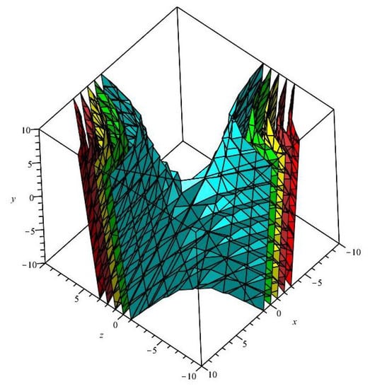
Figure 1.
The level sets of S.
The first and the second fundamental forms of are, respectively,
where . The unit normal vector field is
The mean curvature functions of are the coefficients of the characteristic polynomial of the second fundamental form w.r.t. the first fundamental form (Figure 2), namely
written
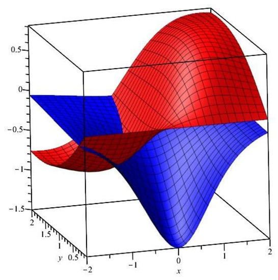
Figure 2.
The first mean curvature function (red) and the second mean curvature function (blue). Notation: , .
We calculate
We represent graphically, separately, the first two mean curvature functions, at large scale (only the zone must be retained from the graphics in Figure 3 and Figure 4).
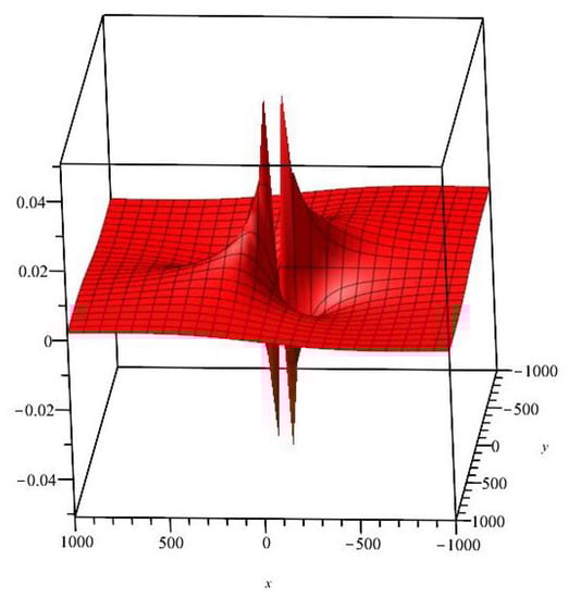
Figure 3.
The first mean curvature function at large scale. Notation: , .
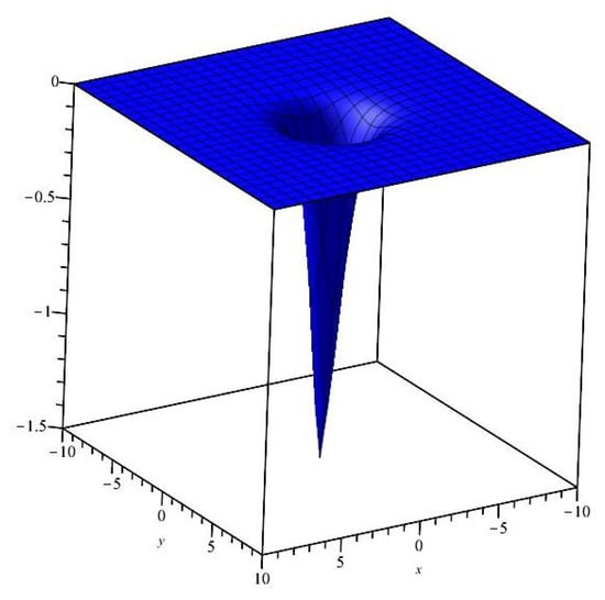
Figure 4.
The second mean curvature function at large scale. Notation: , .
The roots of the previous characteristic polynomial are the principal curvature functions of (Figure 5). We calculate them:
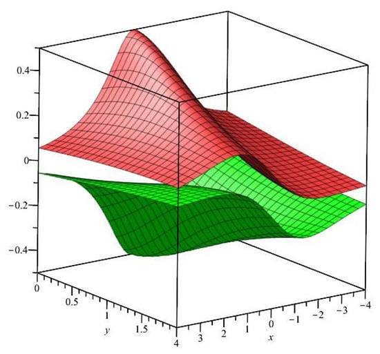
Figure 5.
The first principal curvature function (red) and the second principal curvature function (green). Notation: , .
The mean curvature functions are symmetric expressions of the principal curvature functions. Together (and separately), they “control” the shape of the hypersurface and “measure” how much differs from a hyperplane in .
Proposition 1.
The hypersurface has the following properties:
- (i)
- Its geometric invariants depend on and only.
- (ii)
- It is not minimal, totally geodesic, or totally umbilical. Moreover, it has no umbilical points.
- (iii)
- It has a null, a positive, and a negative smooth principal curvature function. The positive principal curvature function , with equality if and only if . The negative principal curvature function , with equality if and only if .
- (iv)
- It is asymptotically flat.
- (v)
- There do not exist extremal values for , which is unbounded around ; instead, and it has a global minimum at .
The intrinsic Riemannian geometry of can be derived from the first fundamental form only. The Riemannian manifold can be studied in an abstract way, by “forgetting” the embedding of as a hypersurface in . The (non-null) Christoffel symbols are
The geodesics are solutions of the following ODE system:
which may be written in detailed form:
Locally, the geodesics minimize the length of the curves with common ends. Globally, the geodesics behavior is related, in a subtle way, with curvature properties.
Remark 4.
(i) By contrast with the mean and the principal curvature formulas, the previous ODE system depends (formally) on the variable .
(ii) Any geodesic is uniquely determined by two initial conditions: the starting point and its velocity through it. Numerically solving ODE system (14), with initial conditions
and
respectively, produces the geodesics in Figure 6 and Figure 7.
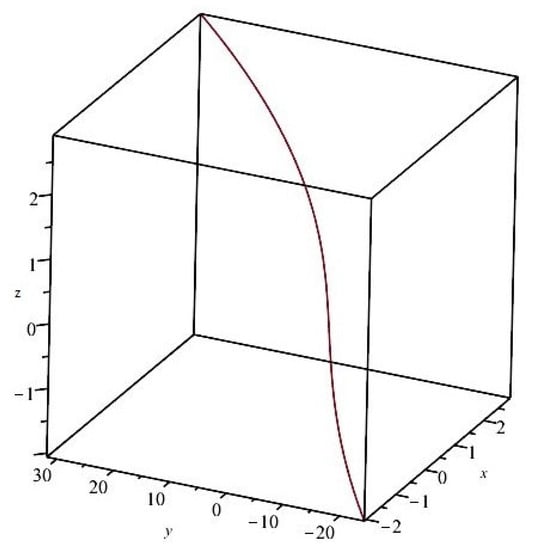
Figure 6.
The first geodesic. Notation: , , .
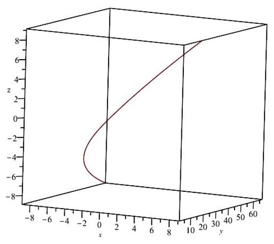
Figure 7.
The second geodesic. Notation: , , .
(iii) As the ODE system (14) is non-linear, integrating it for exact solutions is a difficult task. We consider only the non-degenerate geodesics. A general result in global Riemannian geometry assures us that all geodesics are complete ([57], p. 149, Cor.2.10). It follows that any two points of can be joined by a minimizing geodesic.
A first family of geodesics is of the form
where , , , and are arbitrary constants, with . Another analogous family of geodesics is
where , , , and are arbitrary constants, with .
Suppose and cannot be null on some open interval of the real line. Then, we have another family of geodesics, with ; the function must satisfy an implicit equation of the form
where , are arbitrary constants. The second component of the geodesics can be recovered from the second equation in (14), as the anti-derivative
The variable will depend on two other arbitrary constants.
We calculate now the (non-null) (0,4)-Riemann curvature coefficients,
the (non-null) Ricci coefficients,
and the scalar curvature,
The scalar curvature function is “a trace of a trace” object, obtained by contracting the Riemann curvature tensor field twice. As a “mean of a mean”, is contains information about how bends, but this information is somehow encoded twice. The eventual “reverse engineering” process is difficult; this is why finding Riemannian manifolds with prescribed properties of the scalar curvature functions is challenging.
Proposition 2.
The scalar curvature of is asymptotically flat, and is bounded . Its unique global minimum point is (0, 0, 0) and . Moreover, .
Due to the last property, the graph of the scalar curvature is very similar to the graph of the second mean curvature, and we do not represent it in a separate figure. More interesting seems to be the foliation of by its level sets, which are cylinders along the axis. Points on a fixed leaf correspond to thermodynamic measurements characterized by “linear/longitudinal” heat capacity () and “circular/transversal” thermal pressure () coefficient and volume ().
It must be stressed that the geometry of may also have an interest per se; as stated previously, it is difficult to construct examples of Riemannian manifolds with prescribed properties of the scalar curvature function. In this case, the foliation by cylinders induced by the level sets of the scalar curvature provides exactly such a remarkable example (Figure 8).
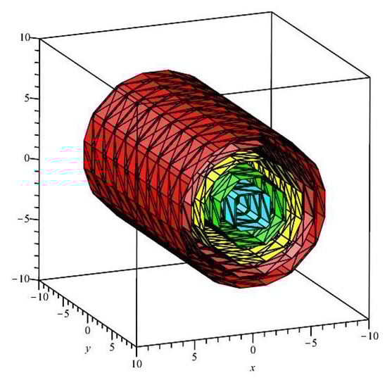
Figure 8.
The level sets of . Notation: , , .
4. Characterization of the Equivalence between the GH Entropy and the BGS, the Tsallis, and the Kaniadakis Entropy
Consider a thermodynamical system as in Section 3. Let M be an open set in , be a parameterized family of probability distributions (PDFs), , with , .
Postulate of entropy equivalence.
We suppose that the GH entropy coincides with the BGS entropy. (For simpler calculations, the Boltzmann constant is normalized to 1).
This property is characterized by the following equivalence equation:
The first two terms describe the GH entropy (via the formalism in Section 3); the (minus) integral is the BGS entropy associated to f. This stochastic integral equation may be useful when we want to determine an unknown PDF f, suitable for a given thermodynamic model. It may act as a bridge between the classical (deterministic) setting and the statistical one.
Example 1.
Let
and an arbitrary real valued function , defined on . Consider the family of parameterized normal PDFs on the real line, given by
A short calculation shows that f is a solution of Equation (15). We remark that the means may depend arbitrarily on the thermodynamic variables. Instead, the dispersion depends inversely proportionally on the GH entropy function.
Similar solutions of Equation (15) may be looked for w.r.t. other generalized logarithms, instead of the Neperian one. The next two examples use the Tsallis logarithm and the Kaniadakis logarithm, respectively.
Example 2.
We look for solutions for the equivalence equation
which is the analogue of Equation (15), where the BGS entropy and the Neperian logarithm were replaced by the Tsallis entropy and the Tsallis q-logarithm ([41])
Suppose and let
and an arbitrary real valued function , defined on . Consider the family of parameterized normal PDFs on the real line, given by (17). One verifies easily, by a direct calculation, that f is a solution of Equation (18). We remark that the means may depend arbitrarily on the thermodynamic variables. The dispersion depends on the GH entropy function in a more subtle way than in Example 1.
When , some (entropy) integrals in (18) may become divergent and the previous reasoning does not work anymore.
Example 3.
We look now for solutions for the equivalence equation
which is the analogue of Equation (15), where the BGS entropy and the Neperian logarithm were replaced by the Kaniadakis entropy and the Kaniadakis k-logarithm ([41])
Consider
and an arbitrary real valued function , defined on . Consider the family of parameterized normal PDFs on the real line, given by (17). A similar calculation proves f is a solution of Equation (20). We remark that the means may depend arbitrarily on the thermodynamic variables. The dispersion depends on the GH entropy function, but in a more complicated way than in Examples 1 and 2.
Remark 5.
(i) The previous three examples suggest the following natural question: Which are the families of PDFs F (not necessarily normal !) and the generalized “logarithms” φ ([41]), such that
This equation establishes the equivalence of the thermodynamic entropy given by the first two terms and the (statistical) generalized entropy associated to the generalized “logarithm” φ. Solving it is much more difficult, as the unknowns are both deterministic (φ) and stochastic (F).
In a previous remark, we explained why we consider only the classical GH equation, and not a generalized one. In the case of generalized GH equations, the first two terms in (22) are to be replaced by another expression in, eventually, more generalized coordinates (corresponding to more thermodynamic state functions and possibly other statistical quantities). The nature of the problem remains unchanged; all complications arise only as a consequence of the complexity of calculations in a space with more dimensions.
(ii) Recently ([52,53]), Gao at al. proved that, under three specific assumptions (of physical inspiration), the only PDF in which the GBS entropy equals the (classical) thermodynamic entropy is the generalized Boltzmann distribution (i.e., a distribution of exponential type). A hint points out that the result may be extended to include the Tsallis entropy as well. This remarkable result gives a partial answer to problem (22).
However, the three assumptions of Gao significantly restrict (from the mathematical perspective) the framework, and weaker hypotheses are desirable. Moreover, hidden necessary conditions exist behind Equation (22), such as the extensivity property; it follows that the thermodynamic entropy and the statistic entropy (equal to the previous one) must be both extensive or both non-extensive (e.g., for the Tsallis and Kaniadakis entropies [58]).
(iii) We must make a clarification of terminology. Common language identifies “entropy” as a functional defined of the set of PDFs, with “entropy” as a specific value of this functional. (At a more elementary level, this happens when we speak about “the function ”, instead of “the function ”).
Denote the BGS, the Tsallis, and the Kaniadakis entropy functionals with , , and , respectively. Denote by , , the parameterized families of PDFs obtained in the three previous examples. We showed that the thermodynamic entropy coincides (as a function of x) with , and . This does not mean that S (which is a function!) coincides with the functionals (!) , , . This is the true meaning of the equivalence stated in (15) and (22).
Remark 6.
Denote a family of PDFs on , φ a generalized logarithm [59] and
a parameterized family of arbitrary generalized entropy functionals. In particular, φ may be any of the Neperian, the Kaniadakis, or the Tsallis logarithms previously considered. Denote a Riemannian generalized Fisher metric on , canonically associated to H and f [41].
The thermodynamic entropy S is called metrically equivalent with the entropy if the first fundamental form g in (10) coincides with . Variants may include the following:
- g and are homothetic;
- g and are conformal;
- g and are in geodesic correspondence.
The new “equivalence problem” can now be stated: Find H and f such that S is metrically equivalent with .
This equivalence of entropies is not more general than the previous one in (22), nor an extension or a particularization of it; it is of a different nature, a kind of intermediate equivalence by means of derived objects. The equivalence in (22) and the “metrical equivalence” are logically unrelated. We do not enter into further detail here, as the study requires the whole machinery behind the generalized Fisher metrics [41].
5. Thermodynamic Interpretations and Applications
The previous sections were more mathematically oriented. Now, we will focus on some physical interpretations of the holonomic model from Section 3 and Section 4. Because our claims may seem too speculative to some physicists, we encourage criticism and reasoned rebuttals.
- (i)
- First, we remark that we use somehow atypical variables, as coordinates for the “space of configurations” (in addition to the volume , which is commonly and frequently used), namely the thermal pressure coefficient and the thermal capacity . However, even if these variables/observables are less common in the literature, they are not completely absent (e.g., [60,61]).As a consequence, the results and the conclusions we obtained are not covariant, because they rest in an essential manner on the particular chosen coordinates system.
- (ii)
- The intrinsic geometry and the extrinsic geometry of the hypersurface do not depend on the variable , so they are independent of the heat capacity . Instead, the set properties of this hypersurface depend on . The hypersurface may have set theoretic or differential properties which cannot be explained geometrically.On another hand, a challenging question is the following: What thermodynamical properties may be characterized through intrinsic properties of and what through extrinsic ones? For example, as remarked previously, optimal paths joining two given states can be modeled as geodesics, which are intrinsic objects.
- (iii)
- Our formalism may be useful when one develops a calculus on the hypersurface , for example, by taking higher-order derivatives of the pressure w.r.t. temperature (see [62] for second-order ones). Geometrization of higher-order derivatives involves, in general, the use of fiber bundles over a manifold; here, the holonomy of the model proves again its superiority over an eventual non-holonomic model, where the manifold machinery is weaker.
- (iv)
- Translations can be made between geometric and physical properties. For example, the only points where the first mean curvature function vanishes are the critical points for the pressure function (w.r.t. the temperature); the minimum value for and the “unbounded” behavior of arise only for extreme physical conditions (very small volume and thermal pressure coefficient).
The intersection curve of the two level sets satisfies the system of two implicit equations and an inequation
There exists a unique , such that
The parameterized intersection curve has the graph in Figure 9.
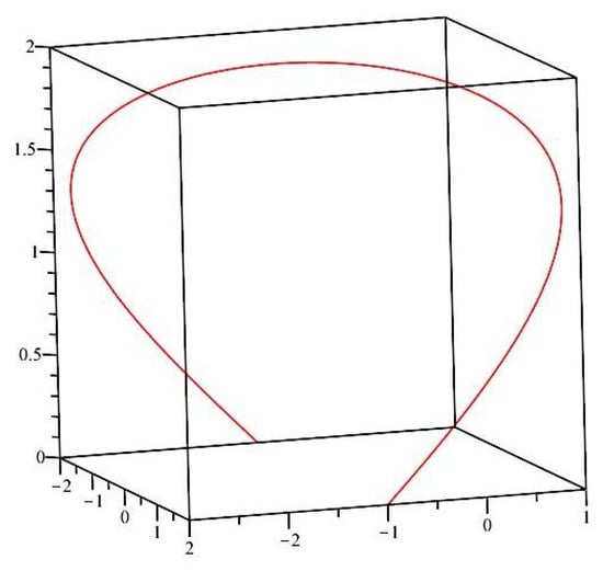
Figure 9.
The intersection of the two level sets.
The second coordinate of the intersection curve (which corresponds to the heat capacity restricted along the intersection curve) suggests a point
situated on a virtual circle of center and radius . Formally, we denote and call it the mate heat capacity along the intersection curve. The following formula holds:
We do not know if this quantity can be extended to a (formal, speculative, and exotic) new state variable; anyhow, it has an interesting intrinsic interpretation.
- (v)
- The parameterized PDFs, which arise as solutions of the special stochastic equations in Section 4, are encountered in the literature, in different frameworks (see, for example, [63]). Moreover, the geometrization of such parameter spaces leads to the study of statistical manifolds and of Fisher-like Riemannian metrics in information geometry (see [39,40,41] and reference therein).
- (vi)
- The ODE system (14) allows the determination of the geodesics lying on the hypersurface . As pointed out in Remark 4 (iii), any geodesic local minimizes the arc length between two points, which can be interpreted as two events in the space of thermodynamic states , , , and S. We have here a possible control tool, useful to “drive” a thermodynamic engine from a starting state to a nearby final state.
More precisely, consider the “state” in at time , characterized by , , and . We want to reach the “state” , by the “shortest” path. Remark 4, (iii) ensures us that there exists a unique “minimal” geodesic
such that . Here, “minimal” refers to the Riemannian distance w.r.t. the first fundamental form, not to the Euclidean distance (as the coordinates are not position coordinates). In practice, the geodesic must be determined numerically, from (14).
Such an approach is, of course, determined/limited by the choice we made, by the particular Riemannian geometry we found on . There exist other alternative Riemannian metrics with similar claims ([64,65,66]), associated to the GH equation, and a comparison of their practical efficiency and relevance deserves another detailed study.
- (vii)
- The maximum entropy (MaxEnt) problem is a fundamental area of investigation in Statistical Mechanics and information theory. Its classical thermodynamics counterpart is less studied and, in any case, with totally different tools ([67], Ch.5); mathematical optimization with non-holonomic constraints is a difficult theory, which emerged only recently (see [68,69,70] and references therein).Our holonomic geometrization allows a direct study, with geometric visualization, of (thermodynamic) entropy fluctuations, including extremum points, on subsets of the hypersurface .
- (viii)
- The geometric model in Section 3 does not take into account the (eventual) positiveness of the entropy. Such an additional condition, if necessary, restricts the framework to an open set of .
- (ix)
- Like other fundamental equations in physics, the GH equation does not remain valid outside “normal conditions”, for example, for long-range interactions. Our holonomic model in Section 4 can be refined to cover scale fluctuations. As the coordinates we use are not the “spatial” ones, the Euclidean distance r (such as the length of the position vector field in spherical coordinates) no longer has applicability. We replace the r-scale by the V-scale, because there is a direct (nonlinear) proportionality between them.
Let be a smooth function, strictly increasing, with the following properties:
Obviously, there exists a unique such that . Relevant examples are , for a fixed positive ; , for fixed positive b and .
Consider the ν-GH equation
We derive the formula for the ν-entropy
In particular, for , we obtain and we recover Formula (6).
By analogy with the computations in Section 3, we obtain a hypersurface , we derive a first fundamental form , a second fundamental form , the mean curvature functions, the principal curvature functions, and the scalar curvature function, and we can write the equations of the geodesics.
Each member of this infinite family of models “parameterized” by deserves a similar study as those in Section 4 and Section 5. The techniques will be similar but with distinctive outcomes. At “infinity” will dominate the long-range interactions with specific (local) entropies; near “zero”, for tiny-range interactions, we shall obtain different specific entropies.
- (x)
- The non-holonomic character of the Gibbs–Helmholtz Equation (2) (or its equivalent counterpart (1)) obstructs the description of solutions as global integral hypersurfaces in . Moreover, the versatility of the theromdynamics formalism and “idioms” hides an apparent paradox; the phase functions G, p, S, T, V depend on each other, but, when considered as coordinates, they are supposed to be independent. This is why, in the literature, one often uses a particular (and implicit) case; the Gibbs internal energy G is supposed to be a function of the temperature and pressure only, i.e., . This loss of generality seems a fair price to pay, but (unfortunately) there are more hidden additional “taxes”. For example, from (2) and (6), one derives and ; it follows that the thermal pressure coefficient is always null!
Of course, all our previous results work also in the special case , where they are significantly simplified.
6. Discussion
The first part of the paper contains a short incursion into the realm of non-holonomic geometrizations of GH equations. We did not intend to develop this path, because comparing the possible approaches and further studies would take too much space. This may be an interesting project for the future. The same remark is valid for an eventual critical study about the pros and the cons of the non-holonomic modelization, when compared to the holonomic one.
The results in Section 4 originate in our belief that entropy must be described in a unified way in Classical Thermodynamics, as in statistical mechanics or information theory. We avoided the temptation to postulate it firmly, because we are aware that this hypothesis might look too speculative, from the viewpoint of both theoretical or applied scientists. Our mathematical results are expressed in a neutral approach, leaving open doors toward unlimited future conclusions. The powerful local and global differential geometric tools and, especially, the Riemannian machinery, may bring new insights concerning the abstract “phase spaces” from thermodynamics. A more ambitious goal would be a (differential geometry-based) “Grand Unifying Theory” for thermodynamics, to include the non-holonomic models for the GH equation, the holonomic ones (as such in Section 3), and—eventually—the statistical manifolds approach [39,40].
In addition to the content of Section 4 and Section 5, more physical interpretations are needed, in order to confirm or to reject our claims. We must investigate if our speculative ideas correspond not only to (possible) “gedanken experiments”, but also to real life thermodynamic systems with significant applications. For example, it would be interesting to know if the geodesic movement on the hypersurface corresponds to the most efficient path into the “phase space” of a thermodynamic system.
Developments may include solving the analogue of Equations (15), (18), and (20), for other remarkable families of entropies (Renyi, Sharma–Taneja–Mittal, Naudts, etc). New examples are needed, in addition to the PDF solutions of normal type ([71,72,73,74]). Rethinking the basic thermodynamics postulates may, in particular, impose restrictions on the “equivalence problem” for entropy and forbid some PDFs to be solutions.
Equations (7)–(9) can be used in order to construct similar holonomic geometrizations of the GH equation. In these cases, one needs a completely different approach to characterize the equivalence of the GH entropy and entropies from statistical mechanics (BGS, Tsallis, Kaniadakis, etc). Instead of the “simple” stochastic integral equivalence in Equations (17), (20), and (22), one presumably will obtain more complicated stochastic functional and integral equivalence equations.
We restricted our study to the physics domain, but we must stress that there exists another active field of research, which translates (via a specific dictionary) the thermodynamical notions and results into economic ones [49,50,51,75,76]. For example, the internal energy, the temperature, and the pressure are translated to the growth potential, the internal politics stability, and the price level, respectively; the entropy conserves its meaning. All the contents of our paper have a direct correspondence within this economic theory, which remains to be more precisely developed in a future paper.
In several places in the paper, we emphasized the multitude of Riemannian geometries which can be associated, in various ways, to holonomic or to non-holonomic models for the GH equation. There exist at least two tools to compare any two such geometries. The first one is by means of the deformation algebra associated to the Levi–Civita connections of the respective Riemannian metrics (see [77] and references therein). The second one is the geodesic correspondence, which eventually occurs between two Riemannian manifolds and can translate the geodesic dynamics from one space into the other (see, for example, [78]). The comparison results are important in differential geometry, as they establish sufficient (and sometimes also necessary) conditions, in order that a “space” be homeomorphic, diffeomorphic, isometric, conformal, etc., with a standard one (for example, a plane or a sphere). The deformation results establish “how far” a ”space” is from a standard one.
7. Conclusions
The paper reviews some known non-holonomic geometric tools and develops some new holonomic ones, in order to model the solutions of the Gibbs–Helmholtz equation from thermodynamics. Beyond the mathematical results, at the border of differential geometry with statistics, we make some speculative claims about possible applications in physics and in information theory. The key notion is the use of entropy, through both the classical and the statistical approaches. This combined study is facilitated by the choice of a new coordinate system in the phase space , parameterizing the entropy as a function depending on the thermal pressure coefficient, the heat capacity, and the volume.
Author Contributions
Conceptualization, C.-L.P., I.-E.H., G.-T.P. and V.P.; methodology, C.-L.P., I.-E.H., G.-T.P. and V.P.; validation, C.-L.P., I.-E.H., G.-T.P. and V.P.; writing—original draft preparation, C.-L.P., I.-E.H., G.-T.P. and V.P.; writing—review and editing, C.-L.P., I.-E.H., G.-T.P. and V.P.; visualization, C.-L.P., I.-E.H., G.-T.P. and V.P. All authors have read and agreed to the published version of the manuscript.
Funding
This research received no external funding.
Data Availability Statement
No new data were created.
Acknowledgments
The authors dedicate this paper to the memory of their teacher and colleague, Liviu Constantin Nicolescu (1940–2023), professor emeritus at the University of Bucharest.
Conflicts of Interest
The authors declare no conflict of interest.
References
- Akih-Kumgeh, B. Toward Improved Understanding of the Physical Meaning of Entropy in Classical Thermodynamics. Entropy 2016, 18, 270. [Google Scholar] [CrossRef]
- Ansermet, J.-P.; Brechet, S.D. Principles of Thermodynamics; Cambridge University Press: Cambridge, UK, 2019. [Google Scholar]
- Atkins, P. The Laws of Thermodynamics: A Very Short Introduction; Oxford University Press: Oxford, UK, 2010. [Google Scholar]
- Popovic, M.E. Research in Entropy Wonderland: A Review of the Entropy Concept. Therm. Sci. 2018, 22, 1163–1178. [Google Scholar] [CrossRef]
- Saggion, A.; Faraldo, R.; Pierno, M. Thermodynamics; Springer: Cham, Switzerland, 2019. [Google Scholar]
- Mander, P. Available online: https://carnotcycle.wordpress.com/ (accessed on 13 September 2023).
- Bawden, D.; Robinson, L. “A few exciting words”: Information and entropy revisited. J. Assoc. Inf. Sci. Technol. 2015, 66, 1965–1987. [Google Scholar] [CrossRef]
- Flores Camacho, F.; Ulloa Lugo, N.; Covarrubias Martınez, H. The concept of entropy, from its origins to teachers. Rev. Mex. Fis. 2015, 61, 69–80. [Google Scholar]
- Carnap, R. Two Essays on Entropy; University of California Press: Berkeley, CA, USA; Los Angeles, CA, USA, 1977. [Google Scholar]
- Dieks, D. Is There a Unique Physical Entropy? Micro Versus Macro. In New Challenges to Philosophy of Science. The Philosophy of Science in a European Perspective; Andersen, H., Dieks, D., Gonzalez, W., Uebel, T., Wheeler, G., Eds.; Springer: Dordrecht, The Netherlands, 2013; Volume 4. [Google Scholar]
- Feistel, R. Distinguishing between Clausius, Boltzmann and Pauling Entropies of Frozen Non-Equilibrium States. Entropy 2019, 21, 799. [Google Scholar] [CrossRef]
- Gaudenzi, R. Entropy? Exercices de Style. Entropy 2019, 21, 742. [Google Scholar] [CrossRef]
- Gujrati, P.A. On Equivalence of Nonequilibrium Thermodynamic and Statistical Entropies. Entropy 2015, 17, 710–754. [Google Scholar] [CrossRef]
- Jauch, J.M.; Baron, J.G. Entropy, Information and Szilard’s Paradox. Helv. Phys. Acta 1972, 45, 220–232. [Google Scholar]
- Jaynes, E.T. Gibbs vs. Boltzmann Entropies. Am. J. Phys. 1965, 33, 391–398. [Google Scholar] [CrossRef]
- Kostic, M.M. The Elusive Nature of Entropy and Its Physical Meaning. Entropy 2014, 16, 953–967. [Google Scholar] [CrossRef]
- Lynskey, M.J. An Overview of the Physical Concept of Entropy. J. Glob. Media Stud. 2019, 25, 1–16. [Google Scholar]
- Majernik, V. Entropy-A Universal Concept in Sciences. Nat. Sci. 2014, 6, 552–564. [Google Scholar] [CrossRef]
- Maroney, O.J.E. The Physical Basis of the Gibbs-von Neumann entropy. arXiv 2008, arXiv:0701127v2. [Google Scholar]
- Marques, M.S.; Santana, W.S. What is entropy?—Reflections for science teaching. Res. Soc. Dev. 2020, 9, e502974344. [Google Scholar] [CrossRef]
- Plastino, A.; Curado, E.M.F. Equivalence between maximum entropy principle and enforcing dU=TdS. Phys. Rev. 2005, 72, 047103. [Google Scholar]
- Prunkl, C.E.A.; Timpson, C.G. Black Hole Entropy is Thermodynamic Entropy. arXiv 2019, arXiv:1903.06276v1. [Google Scholar]
- Prunkl, C. On the Equivalence of von Neumann and Thermodynamic Entropy. Philos. Sci. 2020, 87, 262–280. [Google Scholar] [CrossRef]
- Serdyukov, S.I. Macroscopic Entropy of Non-Equilibrium Systems and Postulates of Extended Thermodynamics: Application to Transport Phenomena and Chemical Reactions in Nanoparticles. Entropy 2018, 20, 802. [Google Scholar] [CrossRef]
- Swendsen, R.H. Thermodynamics, Statistical Mechanics and Entropy. Entropy 2017, 19, 603. [Google Scholar] [CrossRef]
- Wallace, D. Gravity, Entropy, and Cosmology: In Search of Clarity. Br. J. Philos. Sci. 2010, 61, 513–540. [Google Scholar] [CrossRef]
- Werndl, C.; Frigg, R. Entropy: A guide for the perplexed. In Probabilities in Physics; Beisbart, C., Hartmann, S., Eds.; Oxford University Press: Oxford, UK, 2011; pp. 115–142. [Google Scholar]
- Badescu, V. Modeling Thermodynamic Distance, Curvature and Fluctuations: A Geometric Approach; Springer: Cham, Switzerland, 2016. [Google Scholar]
- Bravetti, A. Contact Hamiltonian Dynamics: The Concept and Its Use. Entropy 2017, 19, 535. [Google Scholar] [CrossRef]
- Entov, M.; Polterovich, L. Contact topology and non-equilibrium thermodynamics. Nonlinearity 2023, 36, 3349. [Google Scholar] [CrossRef]
- Geiges, H. A Brief History of Contact Geometry and Topology. Expo. Math. 2001, 19, 25–53. [Google Scholar] [CrossRef]
- Ghosh, A.; Bhamidipati, C. Contact geometry and thermodynamics of black holes in AdS spacetimes. Phys. Rev. D 2019, 100, 126020. [Google Scholar] [CrossRef]
- Grmela, M. Contact Geometry of Mesoscopic Thermodynamics and Dynamics. Entropy 2014, 16, 1652–1686. [Google Scholar] [CrossRef]
- Kholodenko, A.L. Applications of Contact Geometry and Topology in Physics; World Science Press: Singapore, 2013. [Google Scholar]
- Kycia, R.A.; Ulan, M.; Schneider, E. Nonlinear PDEs, Their Geometry, and Applications; Springer: Cham, Switzerland, 2019. [Google Scholar]
- Mrugala, R. On contact and metric structures on thermodynamic spaces. Rims Kokyuroku 2000, 1142, 167–181. [Google Scholar]
- Schneider, E. Differential Invariants of Measurements, and Their Relation to Central Moments. Entropy 2020, 22, 1118. [Google Scholar] [CrossRef]
- Simoes, A.A.; de Leon, M.; Valcazar, M.L.; de Diego, D.M. Contact geometry for simple thermodynamical systems with friction. Proc. R. Soc. A 2020, 476, 20200244. [Google Scholar] [CrossRef]
- Hirica, I.E.; Pripoae, C.L.; Pripoae, G.T.; Preda, V. Affine differential control tools for statistical manifolds. Mathematics 2021, 9, 1654. [Google Scholar] [CrossRef]
- Hirica, I.-E.; Pripoae, C.-L.; Pripoae, G.-T.; Preda, V. Conformal Control Tools for Statistical Manifolds and for g-Manifolds. Mathematics 2022, 10, 1061. [Google Scholar] [CrossRef]
- Hirica, I.-E.; Pripoae, C.-L.; Pripoae, G.-T.; Preda, V. Weighted Relative Group Entropies and Associated Fisher Metrics. Entropy 2022, 24, 120. [Google Scholar] [CrossRef]
- Nicolescu, L.; Pripoae, G.T. Gheorghe Vrănceanu—Successor of Gheorghe Țițeica at the geometry chair of the University of Bucharest. Balkan J. Geom. Appl. 2005, 10, 11–20. [Google Scholar]
- Vranceanu, G. Les espaces non holonomes. Mémorial Des Sci. Math. 1936, 76, 70. [Google Scholar]
- Vranceanu, G. Leçons de Géométrie Différentielle; Éditions de l’ Académie de la République Populaire Roumaine: Bucharest, Romania, 1936. [Google Scholar]
- Katsurada, Y. On the theory of non-holonomic systems in the Finsler space. Tohoku Math. J. 1951, 2, 140–148. [Google Scholar] [CrossRef]
- Udriste, C. Geometric Dynamics; Kluwer Academic Publication: Dordrecht, Germany, 2000. [Google Scholar]
- Stamin, C.; Udriste, C. Nonholonomic geometry of Gibbs contact structure. U.P.B. Sci. Bull. Series A 2010, 72, 153–170. [Google Scholar]
- Stamin, C.; Udriste, C. Nonholonomic Gibbs hypersurface. B Proc. 2009, 17, 218–228. [Google Scholar]
- Udriste, C.; Tevy, I.; Ferrara, M. Nonholonomic Economic Systems. In Extrema with Nonholonomic Constraints; Udriste, C., Dogaru, O., Tevy, I., Eds.; Geometry Balkan Press: Bucharest, Romania, 2002; pp. 139–150. [Google Scholar]
- Udriste, C.; Ferrara, M.; Opris, D. Economic Geometric Dynamics; Geometry Balkan Press: Bucharest, Romania, 2004. [Google Scholar]
- Udriste, C.; Ciancio, A. Interactions of nonholonomic economic systems. In Proceedings of the 3rd International Colloquium “Mathematics in Engineering and Numerical Physics”, Bucharest, Romania, 7–9 October 2004; Balkan Society of Geometers, Geometry Balkan Press: Bucharest, Romania, 2005; pp. 299–303. [Google Scholar]
- Gao, X.; Gallicchio, E.; Roitberg, A.E. The generalized Boltzmann distribution is the only distribution in which the Gibbs-Shannon entropy equals the thermodynamic entropy. J. Chem. Phys. 2019, 151, 034113. [Google Scholar] [CrossRef] [PubMed]
- Gao, X. The Mathematics of the Ensemble Theory. Results Phys. 2022, 34, 105230. [Google Scholar] [CrossRef]
- Blankschtein, D. Lectures in Classical Thermodynamics with an Introduction to Statistical Mechanics; Springer: Cham, Switzerland, 2020. [Google Scholar]
- Haszpra, T.; Tel, T. Topological Entropy: A Lagrangian Measure of the State of the Free Atmosphere. J. Atmos. Sci. 2013, 70, 4030–4040. [Google Scholar] [CrossRef]
- Abdulagatov, I.M.; Magee, J.W.; Polikhronidi, N.G.; Batyrova, R.G. Internal Pressure and Internal Energy of Saturated and Compressed Phases. In Enthalpy and Internal Energy: Liquids, Solutions and Vapours; Wilhelm, E., Letcher, T., Eds.; Royal Society of Chemistry: Cambridge, UK, 2017; pp. 411–446. [Google Scholar]
- do Carmo, M.P. Riemannian Geometry; Birkhäuser: Boston, MA, USA, 1993. [Google Scholar]
- Umarov, S.; Tsallis, C. Mathematical Foundations of Nonextensive Statistical Mechanics; World Scientific Press: Singapore, 2022. [Google Scholar]
- Clenshaw, C.W.; Lozier, D.W.; Olver, F.W.J.; Turner, P.R. Generalized exponential and logarithmic functions. Comput. Math. Appl. B 1986, 12, 1091–1101. [Google Scholar] [CrossRef][Green Version]
- Chen, Y.; Li, K.; Xie, Z.Y.; Yu, J.F. Cross derivative of the Gibbs free energy: A universal and efficient method for phase transitions in classical spin models. Phys. Rev. 2020, 101, 165123. [Google Scholar] [CrossRef]
- Liu, Y.; Liu, Y.; Drew, M.G.B. Relationship between heat capacities derived by different but connected approaches. Am. J. Phys. 2020, 88, 51–59. [Google Scholar] [CrossRef]
- Ahlers, G. Temperature Derivative of the Pressure of 4He at the Superfluid Transition. J. Low Temp. Phys. 1972, 7, 361–364. [Google Scholar] [CrossRef]
- Elnaggar, M.S.; Kempf, A. Equivalence of Partition Functions Leads to Classification of Entropies and Means. Entropy 2012, 14, 1317–1342. [Google Scholar] [CrossRef]
- Cafaro, C.; Luongo, O.; Mancini, S.; Quevedo, H. Thermodynamic length, geometric efficiency and Legendre invariance. Phys. Stat. Mech. Appl. 2022, 590, 126740. [Google Scholar] [CrossRef]
- Scandi, M.; Perarnau-Llobet, M. Thermodynamic length in open quantum systems. Quantum 2019, 3, 197. [Google Scholar] [CrossRef]
- Zulkowski, P.R.; Sivak, D.A.; Crooks, G.E.; DeWeese, M.R. Geometry of thermodynamic control. Phys. Rev. E 2012, 86, 041148. [Google Scholar] [CrossRef]
- Harte, J. Maximum Entropy and Ecology: A Theory of Abundance, Distribution, and Energetics; Oxford University Press: Oxford, UK, 2011. [Google Scholar]
- Lucia, U.; Grisolia, G. Non-holonomic constraints: Considerations on the least action principle also from a thermodynamic viewpoint. Results Phys. 2023, 48, 106429. [Google Scholar] [CrossRef]
- Udriste, C.; Dogaru, O.; Ferrara, M.; Ţevy, I. Nonholonomic Optimization. In Recent Advances in Optimization; Lecture Notes in Economics and Mathematical Systems; Seeger, A., Ed.; Springer: Berlin/Heidelberg, Germany, 2006; Volume 563, pp. 119–132. [Google Scholar]
- Yoshimura, H.; Gay-Balmaz, F. Hamiltonian variational formulation for nonequilibrium thermodynamics of simple closed systems. IFAC Pap. Online 2022, 55, 81–85. [Google Scholar] [CrossRef]
- Drăgan, M. Some general Gompertz and Gompertz-Makeham life expectancy models. Analele Stiintifice Univ. Ovidius Mat. 2022, 30, 117–142. [Google Scholar]
- Iatan, I.; Drăgan, M.; Dedu, S.; Preda, V. Using Probabilistic Models for Data Compression. Mathematics 2022, 10, 3847. [Google Scholar] [CrossRef]
- Suter, F.; Cernat, I.; Drăgan, M. Some Information Measures Properties of the GOS-Concomitants from the FGM Family. Entropy 2022, 24, 1361. [Google Scholar] [CrossRef] [PubMed]
- Văduva, I.; Drăgan, M. On the simulation of Some Particular Discrete Distributions. Rewiev Air Force Acad. 2018, 16, 17–30. [Google Scholar] [CrossRef]
- Ferrara, M.; Udriste, C. Area Conditions Associated to Thermodynamic and Economic Systems. In Proceedings of the 2nd International Colloquium of Mathematics in Engineering and Numerical Physics, University Politehnica of Bucharest, Bucharest, Romania, 22–27 April 2002; BSG Proceedings 8. Geometry Balkan Press: Bucharest, Romania, 2003; pp. 60–68. [Google Scholar]
- Georgescu-Roegen, N. The Entropy Law and the Economic Process; Harvard University Press: Cambridge, MA, USA, 1999. [Google Scholar]
- Nicolescu, L.; Martin, M. Einige Bemerkungen über die Deformations Algebra. Abh. Math. Sem. Univ. Hamburg 1979, 49, 244–253. [Google Scholar] [CrossRef]
- Nicolescu, L. Sur la représentation géodésique et subgéodesique des espaces de Riemann. An. Univ. București Matem. 1983, XXXII, 57–63. [Google Scholar]


Disclaimer/Publisher’s Note: The statements, opinions and data contained in all publications are solely those of the individual author(s) and contributor(s) and not of MDPI and/or the editor(s). MDPI and/or the editor(s) disclaim responsibility for any injury to people or property resulting from any ideas, methods, instructions or products referred to in the content. |
© 2023 by the authors. Licensee MDPI, Basel, Switzerland. This article is an open access article distributed under the terms and conditions of the Creative Commons Attribution (CC BY) license (https://creativecommons.org/licenses/by/4.0/).