Abstract
This work revisits the number of limit cycles (LCs) in a piecewise smooth system of Hamiltonian with a heteroclinic loop generalization, subjected to perturbed functions through polynomials of degree m. By analyzing the asymptotic expansion (AE) of the Melnikov function with first-order near the generalized heteroclinic loop (HL), we utilize the expansions of the corresponding generators. This approach allows us to establish both lower and upper bounds for the quantity of limit cycles in the perturbed system. Our analysis involves a combination of expansion techniques, derivations, and divisions to derive these findings.
MSC:
34C07; 34C28; 34C05; 37G15
1. Introductory Notes
The theory of limit cycle (LC) bifurcation in piecewise smooth integrable differential systems finds widespread application in numerous practical problems, spanning domains like electronic engineering, neural networks, automatic control, and biological mathematics, among others [1,2]. Additionally, this theory bears relevance to Hilbert’s 16th problem, adding further significance to its exploration. As a result, the investigation of LC bifurcation within differential systems (piecewise smooth) has emerged as a prominent and dynamic area of research in recent years [3,4,5].
The prevalence of natural laws and diverse influencing factors has led to the extensive application of LC bifurcation theory in piecewise smooth integrable differential systems across various practical fields. Engineers often rely on this theory to address complex challenges in electronic engineering, while researchers in neural networks and automatic control also find it instrumental in their work [6,7].
Beyond its wide-ranging applicability, the theory’s connection to Hilbert’s 16th problem and Weakened Hilbert’s 16th problem underscores its fundamental importance in mathematics. Consequently, researchers have increasingly directed their attention toward the study of LC bifurcation within differential systems, recognizing the richness and relevance of this subject. The growing body of work in this area is evident in recent literature, with various studies exploring different aspects and applications [8,9]. As a result, the pursuit of understanding and harnessing the dynamics of LCs in such systems has become a vibrant and active research pursuit, attracting researchers from diverse backgrounds and interests.
Considered the following perturbed piecewise smooth Hamiltonian systems [10,11]:
where
where are perturbation parameters. As long as , the associated Hamiltonian functions to (1) can be written as
and
The unperturbed version of (1) has a family of orbits with periodicity as comes next:
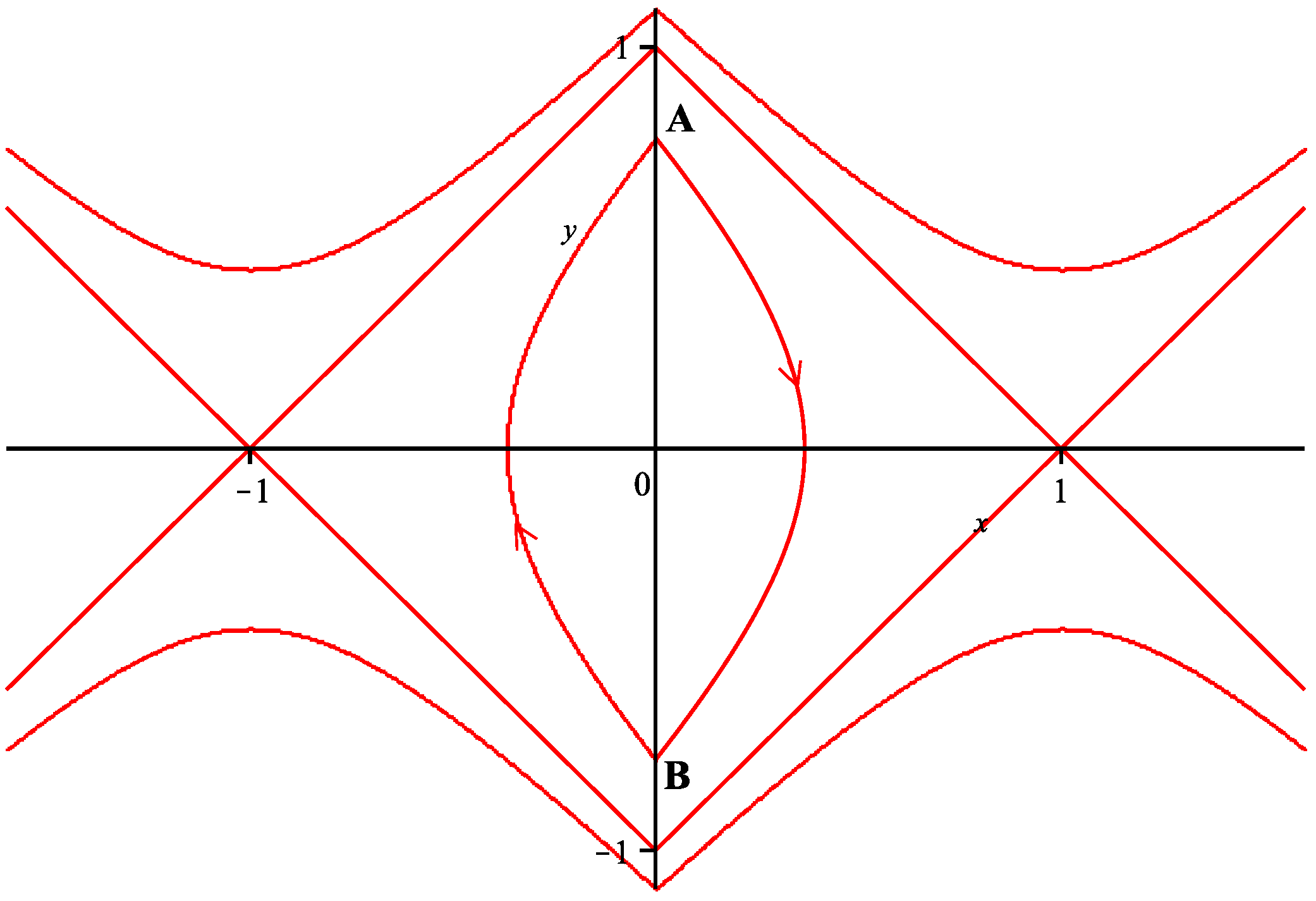
where . The dynamics of the system are characterized by the presence of periodic orbits situated between two key points. Firstly, there is the origin, which serves as an elementary center of the parabolic–parabolic type, see [12,13] for more. Secondly, we observe a generalized heteroclinic loop (HL) encircling the origin, with two saddle points located at . This configuration of periodic orbits is visually represented in Figure 1. Noting that the unperturbed piecewise smooth Hamiltonian [14,15] systems find application in various areas of physics and engineering where dynamical systems exhibit discontinuous behaviors or interactions. These systems can describe physical scenarios where the underlying dynamics switch between different regimes due to certain thresholds or conditions. Examples include mechanical systems with impacts or friction, electrical circuits with switches, and biological systems with abrupt transitions. The unperturbed nature of the system refers to its behavior without any external disturbances, allowing for the study of the inherent dynamics and the effects of the discontinuities or switching on the system’s behavior [16,17]. The system’s behavior is intriguing as it exhibits periodic orbits positioned in a delicate balance between the elementary center at the origin and the encircling generalized HL [18]. At the origin, the dynamics manifest as a parabolic–parabolic type, contributing to the system’s unique characteristics. Meanwhile, the presence of saddle points at within the generalized HL introduces an additional layer of complexity to the system’s behavior. The interplay between these fundamental elements gives rise to the observed periodic orbits, which showcase captivating and intricate trajectories in the phase space. To gain further insights into the system’s dynamics and the significance of these periodic orbits, refer to Figure 1, providing a visual representation of this intriguing phenomenon. Figure 1 encapsulates the captivating phenomenon occurring within the system under study. The figure highlights the existence of periodic orbits that reside in the region between the origin and a generalized HL surrounding the origin. While the origin itself serves as an elementary center of parabolic–parabolic type, the loop features saddle points at , adding a distinct dynamic dimension to the system. As a result, the periodic orbits gracefully navigate this delicate balance between the attractive forces of the origin and the more complex interactions near the saddle points. Understanding the underlying principles governing these orbits is vital for comprehending the system’s overall behavior and offers valuable insights into its practical applications and implications.
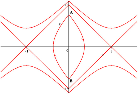
Figure 1.
The phase portrait of (1) in the absence of perturbation (). Choosing for better understanding of the illustration.
By the main results in [19,20], we know that the first order Melnikov function (FOMF) associated with the periodic orbits of (1) as comes next
A fascinating connection exists between the LCs and zeros of the FOMF in the context of system (1). Specifically, the LCs of the system are associated with isolated zeros of the first non-vanishing Melnikov functions (4), see fore more [21,22].
In a related work by Liang and Han [23], they delved into the study of Hopf bifurcation and generalized heteroclinic bifurcation, managing to derive an upper bound for the count of LCs in system (1) up to the first order in . To facilitate their calculations, the authors made simplifications by selecting specific forms for and in each bifurcation case. For the Hopf bifurcation, they used
and set . Noting that in this work , , , and are the perturbation coefficients. On the other hand, for the generalized heteroclinic bifurcation, they employed
and
while .
Li et al. (2016) expanded upon the Melnikov method to address a specific category of perturbed hybrid piecewise smooth systems featuring two switching manifolds in a planar configuration. Their study delved into the continuity of periodic orbits, particularly when the unperturbed system itself possesses such orbits [24]. Other new results about periodic orbits of piecewise smooth systems can be traced in [25,26,27].
In this paper, we take a fresh approach to revisit the problem of LC bifurcation in (1) by considering the more general case of perturbed polynomials and . Unlike the previous study, we do not impose specific constraints on the form of these polynomials, allowing for a more comprehensive exploration of the system’s dynamics.
This paper unfolds with a systematic investigation into the intricate dynamics of the FOMF in Section 2. This section delves into the algebraic properties and underlying structure of , shedding light on its essential characteristics and revealing valuable insights into its behavior. Building upon this foundation, Section 3 embarks on an exploration of the asymptotic expansion (AE) of near pertinent regions of interest. This critical analysis provides a deeper understanding of the function’s behavior and unveils valuable information about its asymptotic properties. More results are obtained because of more general perturbations (general perturbed polynomial differential certain system). Finally, the paper culminates the conclusion in Section 4, summarizing the key findings and implications of the study. Together, these sections present a comprehensive investigation into the intriguing relationship between LCs and the FOMF, contributing to the broader understanding of dynamical systems and bifurcation phenomena.
2. The Algebraic Structure of the FOMF
Our major result consists of the theorem presented below.
Theorem 1.
The count of LCs arising from system (1), originating from the period annulus near the origin and encompassing all valid combinations of and adhering to (2), does not exceed . Additionally, by appropriately selecting the perturbation coefficients , and in the perturbed Equation (1), then (1) can support a total of m LCs.
Toward such a goal, we build several different theoretical findings. Now we investigate the algebraic structure of FOMF for (1). When , we denote
Noting that with respect to the x-axis (s-axis), the orbits are symmetric. Therefore, . The following lemma is now stated and proved.
Lemma 1.
For and when , we have
wherein and are constants and independent of each other. Here, stands for the integer part.
Proof.
Using the Green’s Formula, one has the following
and
By one obtains (7) and (8), one obtains
Hence, can be given by
in view of , where
It is easy to verify that might be chosen as free constants. To continue the proof, we establish the following relations:
where and can be taken as free parameters. Indeed, upon differentiating both sides of with respect to z, one attains
Upon multiplying (11) by the one-form and subsequently integrating, we arrive at the following relation:
Similarly, multiplying both sides by and integrating over , we obtain another relation
Elementary manipulations reduce Equations (12) and (13) to
and
We will now establish the claim using induction on m. To preserve the generality of the argument, we can make the following assumption and move on. We will focus on proving the claim for even values of m (similarly, the claim can be proven for odd values of m). To begin, let us perform a direct computation using the two equalities mentioned above:
Hence, for one has
Indeed, the claim has been verified for . Let us now make the assumption that the claim holds for all values of . Next, by substituting into (2) and into (16), we obtain:
Thus, by leveraging the hypothesis of induction along with (17), one can deduce:
where , , and are constants and (2.6) is proved in view of .
Next, we establish the independence between and . To begin, we utilize the induction hypothesis, which ensures that and are already established as independent. In other words, the determinant of the following Jacobian matrix governs their independence and is not zero
Here, the summation for is less or equal than . This follows directly from the calculations, and we can express the Jacobian matrix as follows:
where is a column vector and is a row vector. We now obtain
which means that and are independent of each other. This completes the proof. □
Before ending this section, it is recalled that the work [28] introduces an extension of the Melnikov function method and the averaging method to study the presence of LCs in piecewise smooth near-integrable systems, even in higher dimensional spaces. Their work demonstrates the equivalence of these methods, which were previously known for planar analytic systems, and establishes their applicability for piecewise systems. That lies in deriving the formula for the second-order Melnikov function in planar piecewise near-Hamiltonian systems.
3. The Asymptotic Expansion of
In this section, our focus shifts towards providing the essential asymptotic expansions of the FOMF in close proximity to both the generalized HL and the origin. These expansions offer valuable insights into the behavior of within these critical regions and lay the groundwork for a deeper understanding of the system’s dynamics.
To begin, let us explore the AE of near the generalized HL . By employing appropriate mathematical techniques, we derive expressions that shed light on the intricate relationship between and . The obtained expansions reveal how the Melnikov function behaves as h approaches and provide valuable information about the system’s response to perturbations in this particular region. Understanding the behavior of near is crucial for comprehending the system’s stability and the emergence of LCs in this vicinity.
Next, we direct our attention to the AE of near the origin. Employing rigorous mathematical analysis, we unveil the behavior of as it approaches the origin. The obtained expansions offer valuable insights into the system’s dynamics in the vicinity of this critical point and provide a deeper understanding of the underlying mechanisms governing LC bifurcations. By unraveling the intricate relationship between and the origin, we gain essential knowledge about the stability and behavior of the system for perturbations close to the origin.
Following the presentation of the asymptotic expansions, we introduce a key lemma that contributes to our understanding of the system’s behavior in the region where . The lemma provides an explicit AE of , a vital component of the Melnikov function, as h approaches the neighborhood of . This expansion, expressed in terms of real constants and , with , illuminates the intricate characteristics of and its relationship with h in this specific region. Such detailed insights into the behavior of contribute significantly to the overall understanding of the Melnikov function and its role in LC bifurcations near .
Lemma 2.
The AE of for are
where , and are real constants.
Proof.
Lemma 3.
For and , the following expansions hold:
wherein and are scalars for and , , ⋯, , , , ⋯, can be taken as free parameters.
Proof.
A direct calculation gives
where
It is possible now to find that , , ⋯, are independent of each other. In view of , one has for
where are constants and for . The independence of , , ⋯, implies that , , ⋯, can be chosen as free constants. Similarly, we can demonstrate that , , ⋯, are also free parameters. The independence of and comes from Lemma 1. This completes the proof. □
Proposition 1.
For , the AE of is
where and are independent of each other, moreover
Proof.
At this moment, we are in a position to establish the major finding of this work using the obtained theoretical findings in what follows.
Proof of Theorem 1
By Proposition 1, we know that and are independent of each other. We can select them in such a way that they read the conditions below:
These conditions imply that in (27) has simple and distinct zeros in . Consequently, system (1) can exhibit m LCs for . Now, our objective is to determine the upper bound for the number of LCs of system (1). To achieve this, we begin with some preliminary considerations.
After performing direct computation, we attain
Thus, we can equivalently write
using the above equality, where are constants. Differentiating (27) times using Lemma 3 furnishes us:
Therefore, has at most zeros on . Observe that , which implies that can have a maximum of zeros on the interval . This conclusion establishes the proof of Theorem 1.
4. Concluding Summaries
In this work, we have investigated the bifurcations and stability of LCs in a general perturbed polynomial differential system (1). Our main focus was on understanding the impact of perturbation parameters on the existence and number of LCs in the system.
In Section 2, we studied the algebraic structure of the FOMF for the system (1). By appropriately selecting the perturbation coefficients, we showed that the number of LCs can be controlled to be m, which represents an exciting result in the study of perturbed polynomial differential systems. We provided a clear theoretical foundation for this result and proved it rigorously.
In Section 3, we analyzed the AE of the FOMF in two critical regions: near the generalized HL and near the origin. These expansions provided valuable insights into the behavior of in these regions and its relation to the underlying dynamics of the system. Additionally, we introduced a key Lemma 2 that presented an explicit AE of , which plays a significant role in the Melnikov function near the value . The obtained results contributed significantly to our understanding of the system’s stability and the emergence of LCs in these critical regions.
In conclusion, our work sheds light on the rich dynamical behavior of perturbed polynomial differential systems and provides a deeper understanding of their stability and bifurcation properties. The findings presented in this work contribute to the existing body of knowledge in the field of dynamical systems theory and can be applied to a wide range of real-world applications, including engineering, physics, and biology.
Future research in this area could explore the behavior of LCs and stability in higher-dimensional perturbed polynomial systems, as well as investigate the effects of other types of perturbations on the system’s dynamics. Additionally, numerical simulations could be conducted to validate and further explore the theoretical findings presented in this paper.
Author Contributions
Conceptualization, E.Z.; formal analysis, E.Z. and S.S.; funding acquisition, S.S.; investigation, E.Z.; methodology, E.Z. and S.S.; supervision, E.Z. and S.S.; validation, E.Z. and S.S.; writing—original draft, E.Z. and S.S.; writing—review and editing, E.Z. and S.S. All authors have read and agreed to the published version of the manuscript.
Funding
This work was supported by NSFC (12161069), the Key Program of Higher Education of Henan (21A110023), Natural Science Foundation of Ningxia (2022AAC05044), The Innovation Studio for Model Workers and Craftsmen Talents of the Education, Science, Culture, Health and Sports of Henan ([2021] No. 21) and The Key Cultivation Project for Academic and Technical Leaders of Zhengzhou College of Finance and Economics (ZCFE[2021] No. 20).
Institutional Review Board Statement
Not applicable.
Informed Consent Statement
Not applicable.
Data Availability Statement
In regard to the data availability statement, we affirm that data sharing is not applicable to this article, as no new data were generated during the course of this study.
Acknowledgments
We would like to thank four anonymous referees for several comments and corrections on an earlier version of this work.
Conflicts of Interest
The authors affirm that they have no known personal relationships or competing financial interests that could have potentially influenced the work reported in this article.
References
- Di Bernardo Laurea, M.; Champneys, A.R.; Budd, C.J.; Kowalczyk, P. Piecewise-Smooth Dynamical Systems. In Theory and Applications; Springer: London, UK, 2008. [Google Scholar]
- Teixeira, M. Perturbation Theory for Non-Smooth Systems. In Encyclopedia of Complexity and Systems Science; Springer: New York, NY, USA, 2009; Volume 22. [Google Scholar]
- Yang, J.; Zhao, L. Bounding the number of limit cycles of discontinuous differential systems by using Picard-Fuchs equations. J. Differ. Equ. 2018, 264, 5734–5757. [Google Scholar] [CrossRef]
- Yang, J.; Zhao, L. Limit cycle bifurcations for piecewise smooth Hamiltonian systems with a generalized eye-figure loop. Int. J. Bif. Chaos 2016, 26, 1650204. [Google Scholar] [CrossRef]
- Yang, J.; Zhao, L. Bifurcation of limit cycles of a piecewise smooth Hamiltonian system. Qual. Theo. Dyn. Sys. 2022, 21, 142. [Google Scholar] [CrossRef]
- Chen, J.; Han, M. Bifurcation of limit cycles by perturbing a piecewise linear Hamiltonian system. Qual. Theory Dyn. Syst. 2022, 21, 34. [Google Scholar] [CrossRef]
- Llibre, J.; Mereu, A.; Novaes, D. Averaging theory for discontinuous piecewise differential systems. J. Diff. Equ. 2015, 258, 4007–4032. [Google Scholar] [CrossRef]
- Ramirez, O.; Alves, A. Bifurcation of limit cycles by perturbing piecewise non-Hamiltonian systems with nonlinear switching manifold. Nonl. Anal. Real World Appl. 2021, 57, 103188. [Google Scholar] [CrossRef]
- Xiong, Y.; Hu, J. A class of reversible quadratic systems with piecewise polynomial perturbations. Appl. Math. Comput. 2019, 362, 124527. [Google Scholar] [CrossRef]
- Sui, S.; Yang, J.; Zhao, L. On the number of limit cycles for generic Lotka-Volterra system and Bogdanov-Takens system under perturbations of piecewise smooth polynomials. Nonl. Anal. Real World Appl. 2019, 49, 137–158. [Google Scholar] [CrossRef]
- Yang, J.; Zhang, E.; Liu, M. Limit cycle bifurcations of a piecewise smooth Hamiltonian system with a generalized heteroclinic loop through a cusp. Comm. Pure Appl. Anal. 2017, 16, 2321–2336. [Google Scholar] [CrossRef]
- Han, M.; Liu, S. Further studies on limit cycle bifurcations for piecewise smooth near-Hamiltonian systems with multiple parameters. J. Appl. Anal. Comput. 2020, 10, 816–829. [Google Scholar]
- Yang, J.; Zhang, E.; Liu, M. Bifurcation analysis and chaos control in a modified finance system with delayed feedback. Int. J. Bifur. Chaos 2016, 26, 1650105. [Google Scholar] [CrossRef]
- Han, M.; Sun, H.; Balanov, Z. Upper estimates for the number of periodic solutions to multi-dimensional systems. J. Diff. Equ. 2019, 266, 8281–8293. [Google Scholar] [CrossRef]
- Archid, A.; Bentbib, A.H. Global symplectic Lanczos method with application to matrix exponential approximation. J. Math. Model. 2022, 10, 143–160. [Google Scholar]
- Gao, Q.; Zhang, E.; Jin, N. The ultimate ruin probability of a dependent delayed-claim risk model perturbed by diffusion with constant force of interest. Bull. Korean Math. Soc. 2015, 52, 895–906. [Google Scholar] [CrossRef]
- Yang, P.; Yu, J. Melnikov analysis in a cubic system with a multiple line of critical points. Appl. Math. Lett. 2023, 145, 108787. [Google Scholar] [CrossRef]
- Zhang, E.; Li, H.; Huang, J. A simple calculation of the first order Melnikov function for a non-smooth Hamilton system. J. Appl. Math. Comput. 2023, 7, 142–146. [Google Scholar] [CrossRef]
- Liu, X.; Han, M. Bifurcation of limit cycles by perturbing piecewise Hamiltonian systems. Int. J. Bifur. Chaos Appl. Sci. Eng. 2010, 20, 1379–1390. [Google Scholar] [CrossRef]
- Han, M.; Sheng, L. Bifurcation of limit cycles in piecewise smooth systems via Melnikov function. J. Appl. Anal. Comput. 2015, 5, 809–815. [Google Scholar]
- Liang, F.; Han, M. Limit cycles near generalized homoclinic and double homoclinic loops in piecewise smooth systems. Chaos Sol. Frac. 2012, 45, 454–464. [Google Scholar] [CrossRef]
- Liang, F.; Han, M.; Romanovski, V. Bifurcation of limit cycles by perturbing a piecewise linear Hamiltonian system with a homoclinic loop. Nonl. Anal. 2012, 75, 4355–4374. [Google Scholar]
- Liang, F.; Han, M. On the number of limit cycles in small perturbations of a piecewise linear Hamiltonian system with a heteroclinic loop. Chin. Ann. Math. 2016, 37, 267–280. [Google Scholar] [CrossRef]
- Li, S.B.; Ma, W.S.; Zhang, W.; Hao, Y.X. Melnikov method for a three-zonal planar hybrid piecewise-smooth system and application. Int. J. Bif. Chaos 2016, 26, 1650014. [Google Scholar] [CrossRef]
- Xie, S.; Han, M.; Zhao, X. Bifurcation of periodic orbits of a three-dimensional piecewise smooth system. Qual. Theory Dyn. Syst. 2019, 18, 1077–1112. [Google Scholar] [CrossRef]
- Pi, D. Periodic orbits for double regularization of piecewise smooth systems with a switching manifold of codimension two. Disc. Cont. Dyn. Sys. B 2022, 27, 1055–1073. [Google Scholar] [CrossRef]
- Li, J.; Guo, Z.; Zhu, S.; Gao, T. Bifurcation of periodic orbits and its application for high-dimensional piecewise smooth near integrable systems with two switching manifolds. Commun. Nonl. Sci. Numer. Simul. 2023, 116, 106840. [Google Scholar] [CrossRef]
- Liu, S.; Hana, M.; Li, J. Bifurcation methods of periodic orbits for piecewise smooth systems. J. Diff. Equ. 2021, 275, 204–233. [Google Scholar] [CrossRef]
Disclaimer/Publisher’s Note: The statements, opinions and data contained in all publications are solely those of the individual author(s) and contributor(s) and not of MDPI and/or the editor(s). MDPI and/or the editor(s) disclaim responsibility for any injury to people or property resulting from any ideas, methods, instructions or products referred to in the content. |
© 2023 by the authors. Licensee MDPI, Basel, Switzerland. This article is an open access article distributed under the terms and conditions of the Creative Commons Attribution (CC BY) license (https://creativecommons.org/licenses/by/4.0/).