Stochastic Multi-Objective Scheduling of a Hybrid System in a Distribution Network Using a Mathematical Optimization Algorithm Considering Generation and Demand Uncertainties

Abstract

In this paper, stochastic scheduling of a hybrid system (HS) composed of a photovoltaic (PV) array and wind turbines incorporated with a battery storage (HPV/WT/Batt) system in the distribution network was proposed to minimize energy losses, the voltage profile, and the HS cost, and to improve reliability in shape of the energy-not-supplied (ENS) index, considering energy-source generation and network demand uncertainties through the unscented transformation (UT). An improved escaping-bird search algorithm (IEBSA), based on the escape operator from the local optimal, was employed to identify the optimal location of the HS in the network in addition to the optimal quantity of PV panels, wind turbines, and batteries. The deterministic results for three configurations of HPV/WT/Batt, PV/Batt, and WT/Batt were presented, and the results indicate that the HPV/WT/Batt system is the optimal configuration with lower energy losses, voltage deviation, energy not supplied, and a lower HS energy cost than the other configurations. Deterministic scheduling according to the optimal configuration reduced energy losses, ENS, and voltage fluctuation by 33.09%, 53.56%, and 63.02%, respectively, compared to the base network. In addition, the results demonstrated that the integration of battery storage into the HPV/WT enhanced the various objectives. In addition, the superiority of IEBSA over several well-known algorithms was proved in terms of obtaining a faster convergence, better objective value, and lower HS costs. In addition, the stochastic scheduling results based on the UT revealed that the uncertainties increase the power losses, voltage deviations, ENS, and HPV/WT/Batt cost by 2.23%, 5.03%, 2.20%, and 1.91%, respectively, when compared to the deterministic scheduling.

1. Introduction

1.1. Motivation

The application of renewable energies, such as photovoltaic (PV) and wind energy, has always attracted the attention of humans due to their abundance and freedom [1]. Despite issues, such as the unpredictable nature of these sources, their reliance on climate change, and their low reliability, making the use of these sources problematic, the proper configuration of these sources in the form of a hybrid system (HS) can mitigate these issues to a large extent [2]. Although the configuration of these systems reduces the reliability problem to a great extent, it makes the optimal and suitable design of such a system difficult [2]. Various storage devices can be added to hybrid energy systems to provide electrical planning based on renewable energy sources. In other words, the load demand is constantly changing and cannot be met over time. On the other hand, hybrid systems without storage elements are not able to continuously supply the load demand because the output of these units is highly dependent on their fluctuating inputs. Among the most common storage devices that are widely used in hybrid energy systems, a battery is a short-term storage form and a hydrogen-based fuel cell is a long-term storage form. Compared to batteries, the use of hydrogen has a higher cost in addition to the problem of its storage under pressure [3]. The use of battery storage can compensate for fluctuations in the production of renewable energy sources (RES) by managing charge and discharge and provide the ability to produce schedulable energy by improving the flexibility of the system [2]. In addition, in recent years, the use of HS in distribution networks has been considered to improve its performance. By using the HS with PV, a wind turbine (WT), and batteries (HPV/WT/Batt), based on the energy management strategy and reserve power management, dispatchable power can be injected into the network even in peak load conditions, thus improving the network performance [4]. This goal is achieved by optimally determining the location and the size of the RES and the charging and discharging pattern of the battery storage [5,6], which requires the use of powerful meta-heuristic algorithms in early convergence conditions; otherwise, in addition to spending huge costs, it also weakens the network performance [7,8].

1.2. Literature Review

Various studies have been conducted in the design of hybrid energy systems, as well as the allocation and planning of the RESs and HSs in distribution networks with different goals and methods. In [9], the sizing of a stand-alone HPV/Diesel/Batt system was performed to minimize the annual cost considering the energy-not-served constraint using a lightning search algorithm. In [10], a social spider optimizer (SSO) was applied to find the optimal size of an HPV/WT/Diesel/Batt system to minimize the cost of energy (COE) satisfying the loss of power supply probability (LPSP). In [11], designing of an off-grid HPV/WT/Batt energy system was developed to achieve the optimal sizing of the system devices using an improved gradient based-optimizer (IGBO) considering cloud theory. In [12], the sizing of a stand-alone HPV/WT/Diesel/Batt system was evaluated using a supply demand-based optimization (SDO) for minimizing the annualized system cost considering the LPSP. In [13], they designed of an off-grid HPV/WT/Diesel/Batt system for minimizing the net present cost, which satisfied the LPSP using an improved Genetic Algorithm (GA). In [14], the sizing of a stand-alone PV/Fuel cell was carried out using the HOMER software to minimize the cost of energy (COE). In [15], an HPV/WT/Batt energy system was optimized to minimize the energy cost considering battery aging to meet the annual demand using opposition-based learning and a gradient-based optimizer (OLGBO). In [16], the optimization of an energy microgrid system is studied considering power conditioning capability to minimize the power losses. In [17], the placement and sizing of CHP for the minimization of power losses and improving the voltage profile and reliability of a distribution network was developed based on the particle swarm optimization (PSO) algorithm. In [18], the allocation of PVs and WTs in a distribution network was performed to minimize its cost and improve its voltage stability using the Thief and Police Algorithm (TPA). In [19], application of the renewable energy resources is studied in the smart grid considering distributed adjustable demand sources to improve the system revenue. In [20], the allocation of PVs in the networks was performed using an improved human learning optimization algorithm (IHLOA) to minimize power losses and improve its voltage profile and stability considering the generation and load uncertainty. In [21], the optimization of a hybrid photovoltaic/wind/fuel cell was implemented using meta-heuristic techniques to constantly supply three typical demands in Kousseri, Cameroon. The determination of the site and size of the PVs and WTs in the distribution network for minimization of the losses and to improve voltage stability using the moth-flame optimizer (MFO) was presented in [21]. In [22], the scheduling of an HPV/WT/Batt system was presented for minimizing its active losses and enhancing its voltage profile using an improved whale optimizer algorithm (IWOA). In [23], the allocation of PVs and WTs was presented in a distribution network based on a probabilistic method using the turbulent flow of water-based optimization (TFWO) considering uncertainty. In [24], the allocation of the WT/Batt system was developed via a modified bald eagle search to minimize the power losses of the distribution network.

A summary of the literature review is presented in

Table 1. Summary of the literature review.

Ref.	HS * Components			Objective Function				UT	Improved Solver
	PV	WT	Battery	Loss	Voltage	Cost	Reliability
[9]	Yes	No	Yes	No	No	Yes	No	No	No
[10]	Yes	Yes	Yes	No	No	Yes	Yes	No	No
[11]	Yes	Yes	Yes	No	No	Yes	Yes	No	Yes
[12]	Yes	Yes	Yes	No	No	Yes	Yes	No	No
[13]	Yes	Yes	Yes	No	No	Yes	Yes	No	Yes
[14]	Yes	No	No	No	No	Yes	No	No	No
[15]	Yes	Yes	Yes	No	No	Yes	Yes	No	Yes
[16]	Yes	Yes	Yes	No	No	Yes	Yes	No	No
[17]	Yes	Yes	Yes	No	No	Yes	Yes	No	No
[18]	Yes	No	No	Yes	Yes	Yes	No	No	No
[19]	Yes	Yes	No	No	Yes	No	Yes	No	No
[20]	Yes	No	No	Yes	Yes	No	No	No	Yes
[21]	Yes	Yes	No	Yes	No	No	Yes	No	No
[22]	Yes	Yes	Yes	Yes	Yes	No	No	No	Yes
[23]	Yes	Yes	No	Yes	No	Yes	Yes	No	No
[24]	No	Yes	No	Yes	No	No	No	No	Yes
This Paper	Yes	Yes	Yes	Yes	Yes	Yes	Yes	Yes	Yes

* HS: Hybrid system, UT: unscented transformation.

. According to the literature review, the research gaps are listed as follows:

−

The review of previous studies showed that most studies have focused on the optimal allocation of photovoltaic and wind resources alone in the network with optimization goals and methods. Also, some studies have installed HPV/WT systems without considering storage in the electrical network. In a few studies, the scheduling of the HPV/WT system was performed with battery storage in the networks.

−

A comprehensive multi-objective function for scheduling the HS in the distribution network has not been well addressed, considering multi-criteria optimization and also considering losses, voltage, cost, and reliability assessments.

−

It was found in the literature review that the meta-heuristic algorithms play a crucial role in optimizing energy system scheduling. However, a meta-heuristic algorithm may not be suitable for solving all optimization problems. The No Free Lunch (NFL) theory [25] suggests the need for powerful algorithms that do not converge prematurely in complex problems. Improvements in algorithms are being made to strengthen performance and avoid getting trapped in local optimums, aiming for more accurate solutions.

−

Moreover, one of the challenges facing the scheduling of the HS in the distribution network is the uncertainty of renewable production as well as the network load, which has made it difficult for the network operators to accurately evaluate the effectiveness of these types of energy systems, as well as the decision-making process, which, considering the uncertainty, can help to solve this challenge.

−

So, the literature review has shown that there is a need to provide a multi-objective framework in the scheduling of the HS, as multi-objective scheduling of the HPV/WT system integrated with battery storage, by providing a comprehensive objective function including minimizing energy losses, voltage deviations, and HS energy costs, plus reliability improvements due to network line outages, using a new improved meta-heuristic algorithm.

1.3. Contributions

The contributions of the paper are described as follows:

−

In this study, an optimal multi-objective scheduling framework is implemented for different configurations of the HS, including the HPV/WT/Batt, PV/Batt, and WT/Batt system, in the network to minimize the energy losses, voltage profile, and the HS energy generation cost, and also to enhance its reliability.

−

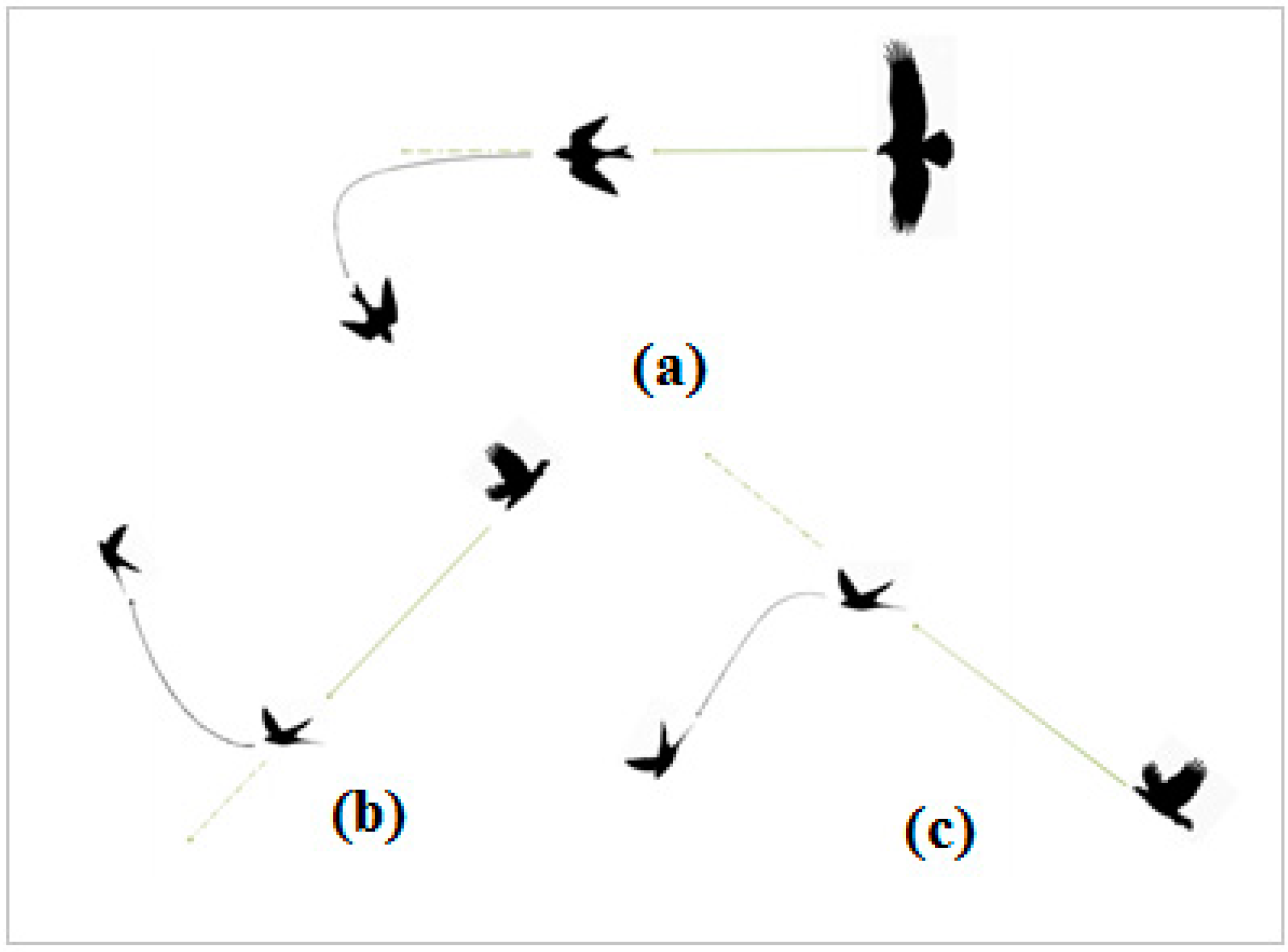
The optimization variables are presented as the site of the HS installation in the distribution network and the size of its components, which are found using a new improved escaping-bird search algorithm (IEBSA). The escape operator from local optimal is used to improve the performance of the conventional escaping-bird search algorithm (EBSA) [26] against premature convergence.

−

The unscented transformation (UT) approach [27] is applied to model the uncertainties, such as renewable generation, and also network load. Compared to the MCS, which is very time consuming, the UT has a low calculation time and no presumptions to simplify the model.

−

The impact of the battery storage considering the reserve energy management and different configurations of the HS is investigated on the scheduling problem and each of the different objectives.

−

The IEBSA performance is compared with traditional EBSA, particle swarm optimization (PSO) [28], and gazelle optimization algorithm (GOA) [29], and its performance in improving each of the objectives is analyzed.

1.4. Paper Structure

The rest of the paper is structured as follows. Objective functions and constraints are presented in Section 2. In Section 3, the HS system modeling is described. The IEBSA and its implementation in scheduling problems are provided in Section 4. The results are given in Section 5 and the findings are presented in conclusion as Section 6.

2. Problem Formulation

The HS system scheduling in the network is formulated in this section.

2.1. Objective Function

The objective function (OF) is presented to minimize the energy losses, voltage deviations, ENS, and HS cost, which is presented as a multi-objective scheduling via the weighted coefficient using the following:

$$\begin{array}{c}{F}_{HS}^{OF}={\psi }_1\times \left(f_{hs1}^{OF}/f_{hs1,\max }^{OF}\right)+{\psi }_2\times \left(f_{hs2}^{OF}/f_{hs2,\max }^{OF}\right)+{\psi }_3\times \left(f_{hs3}^{OF}/f_{hs3,\max }^{OF}\right)\\ +{\psi }_4\times \left(f_{hs4}^{OF}/f_{hs4,\max }^{OF}\right)\end{array}$$

(1)

where, $f_{hs1}^{OF}$, $f_{hs2}^{OF}$, $f_{hs3}^{OF}$ and $f_{hs4}^{OF}$, respectively, indicate the function of energy losses, the voltage deviations, the ENS, and the HS energy generation cost, $f_{hs1,\max }^{OF}$, $f_{hs2,\max }^{OF}$, $f_{hs3,\max }^{OF}$, and $f_{hs4,\max }^{OF}$ are the upper values of energy losses, network voltage deviations, ENS, and HS budget. ${\psi }_1$, ${\psi }_2$, ${\psi }_3$, and ${\psi }_4$ are the weight of objectives such as energy losses, network voltage deviations, the ENS, and the HS cost, and the sum of these coefficients should be 1.

2.1.1. Energy Losses

The first goal of the planning problem is to minimize the energy losses of the network. The energy loss of the network during the study period is calculated by the following [23,24]:

$$f_{hs1}^{OF}={\displaystyle \sum _{t=1}^T{P}_{Loss}(t)}$$

(2)

$$P_{Loss}={\displaystyle \sum _{i=1}^{N_{br}}R{E}_i}\times {\left|\left.C{u}_i\right|\right.}^2$$

(3)

where $R{E}_i$ is ohmic resistance of the line i, and $Cu$ denotes the current of line i.

2.1.2. Voltage Deviation

Minimizing the network voltage fluctuations is the other objective of the scheduling problem. The voltage deviation equation is defined as follows [23,24]:

$$f_{hs2}^{OF}=\sqrt{\frac{1}{N_{bus}}\times {\displaystyle \sum _{i=1}^{N_{bus}}{(Vbu{s}_i-Vbu{s}_p)}^2}}$$

(4)

where Vbus_i denotes ith bus voltage, Vbus_p is the average of buses voltage, and N_bus is the number of buses (here, it was 33).

2.1.3. Reliability

The third objective in solving the HS scheduling problem is to improve the reliability or minimize the energy not supplied (ENS) of the network subscribers due to the lines outage, which is calculated as follows [8]:

$$f_{hs3}^{OF}={\displaystyle \sum _{t=1}^T{\displaystyle \sum _{i=1}^{N_{br}}{\displaystyle \sum _{j=1}^{N_{ld}}{\varphi }_i\times {\partial }_i\times {\Re }_i\times {\Omega }_j}}}$$

(5)

where N_branch is the network line numbers, N_l is load size that is not supplied due to outage of line i, ${\varphi }_i$ is the rate of the ith line outage, ${\partial }_i$ is the length of the ith line, ${\Re }_i$ denotes the repair duration for the fault of the ith line, and ${\Omega }_j$ is the not-provided demand for outage of the ith line.

2.1.4. Cost of HS

The fourth objective is to consider minimizing the cost of the HS including the capital cost and maintenance and operation (O&M) cost, which can be effective in determining the location and component size of the HS in the distribution network, and is calculated as follows [17,24]:

$$f_{hs4}^{OF}=\frac{i{(1+i)}^y}{{(1+i)}^y-1}\times ({\xi }_{PV}^{Cap}+{\xi }_{WT}^{Cap}+{\xi }_{Batt}^{Cap})+({\xi }_{PV}^{O\&M}+{\xi }_{WT}^{O\&M}+{\xi }_{Batt}^{O\&M})$$

(6)

$${\xi }_{PV}^{Cap}=C_{PV,Cap}\times N{u}_{PV}$$

(7)

$${\xi }_{WT}^{Cap}=C_{WT,Cap}\times N{u}_{WT}$$

(8)

$${\xi }_{Batt}^{Cap}=C_{Batt,Cap}\times N{u}_{Batt}$$

(9)

$${\xi }_{PV}^{O\&M}=C_{PV,O\&M}\times N{u}_{PV}$$

(10)

$${\xi }_{WT}^{O\&M}=C_{WT,O\&M}\times N{u}_{WT}$$

(11)

$${\xi }_{Batt}^{O\&M}=C_{Batt,O\&M}\times N{u}_{Batt}$$

(12)

where ${\xi }_{PV}^{Cap}$, ${\xi }_{WT}^{Cap}$ and ${\xi }_{Batt}^{Cap}$ are the capital cost of PVs, WTs and batteries, and ${\xi }_{PV}^{O\&M}$, ${\xi }_{WT}^{O\&M}$ and ${\xi }_{Batt}^{O\&M}$ are the O&M cost of PVs, WTs and batteries, respectively. $C_{PV,Cap}$, $C_{WT,Cap}$, and $C_{Batt,Cap}$ are the cost per PV, WT, and battery unit (with a nominal size of 1 kW, 1 kW, and 1 kAh); $C_{PV,O\&M}$, $C_{WT,O\&M}$, and $C_{Batt,O\&M}$ denote the O&M cost of the PV, WT, and battery unit size (1 kW, 1 kW, and 1 kAh) per year. $N{u}_{PV}$, $N{u}_{WT}$, and $N{u}_{Batt}$ are the number of photovoltaic arrays, wind turbines and batteries, respectively. In Equation (6), $CRF=\frac{i{(1+i)}^y}{{(1+i)}^y-1}$ which CRF is capital recovery factor, i is the annual real interest rate, and y is life span.

2.2. Constraints

The OF is optimized subjected to following equality and inequality constraints [23,24]:

• Power balance constraint

$$\mathrm{A}{\mathrm{P}}_{\mathrm{Post}}+{\displaystyle \sum _{\mathrm{i}=1}^{{\mathrm{N}}_{\mathrm{H}\mathrm{S}}}\mathrm{A}{\mathrm{P}}_{\mathrm{H}\mathrm{S}}(\mathrm{i})=}{\displaystyle \sum _{\mathrm{i}=1}^{{\mathrm{N}}_{\mathrm{b}\mathrm{r}}}\mathrm{A}{\mathrm{P}}_{\mathrm{L}\mathrm{o}\mathrm{s}\mathrm{s}}(\mathrm{i})+{\displaystyle \sum _{\mathrm{q}=1}^{{\mathrm{N}}_{\mathrm{b}\mathrm{u}\mathrm{s}}}\mathrm{A}{\mathrm{P}}_{\mathrm{D}\mathrm{m}\mathrm{d}}(\mathrm{q})}}$$

(13)

$$\mathrm{R}{\mathrm{P}}_{\mathrm{P}\mathrm{o}\mathrm{s}\mathrm{t}}+{\displaystyle \sum _{\mathrm{i}=1}^{{\mathrm{N}}_{\mathrm{H}\mathrm{S}}}\mathrm{R}{\mathrm{P}}_{\mathrm{H}\mathrm{S}}(\mathrm{i})=}{\displaystyle \sum _{\mathrm{i}=1}^{{\mathrm{N}}_{\mathrm{b}\mathrm{r}}}\mathrm{R}{\mathrm{P}}_{\mathrm{L}\mathrm{o}\mathrm{s}\mathrm{s}}(\mathrm{i})+{\displaystyle \sum _{\mathrm{q}=1}^{{\mathrm{N}}_{\mathrm{b}\mathrm{u}\mathrm{s}}}\mathrm{R}{\mathrm{P}}_{\mathrm{D}\mathrm{m}\mathrm{d}}(\mathrm{q})}}$$

(14)

where $\mathrm{A}{\mathrm{P}}_{\mathrm{P}\mathrm{o}\mathrm{s}\mathrm{t}}$ and $\mathrm{R}{\mathrm{P}}_{\mathrm{P}\mathrm{o}\mathrm{s}\mathrm{t}}$ are the injected active and reactive post power to the network, respectively, $\mathrm{A}{\mathrm{P}}_{\mathrm{H}\mathrm{S}}$ and $\mathrm{R}{\mathrm{P}}_{\mathrm{H}\mathrm{S}}$ are the active and reactive HS injected power to the network, $\mathrm{A}{\mathrm{P}}_{\mathrm{L}\mathrm{o}\mathrm{s}\mathrm{s}}$ and $\mathrm{R}{\mathrm{P}}_{\mathrm{L}\mathrm{o}\mathrm{s}\mathrm{s}}$ are network active and reactive losses and $\mathrm{A}{\mathrm{P}}_{\mathrm{D}\mathrm{m}\mathrm{d}}$ and $\mathrm{R}{\mathrm{P}}_{\mathrm{D}\mathrm{m}\mathrm{d}}$ are the active and reactive losses of the network, respectively. N_HS denotes the number of the HS allocated in the network.

• Voltage of the buses

The network buses voltage should be among a certain range [23,24].

$$Vbu{s}_{\min }^i\le Vbu{s}^i\le Vbu{s}_{\max }^i$$

(15)

where $Vbu{s}_{\min }^i$ and $Vbu{s}_{\max }^i$ are the lower and upper value of the buses voltage, respectively. $Vbu{s}_{\min }^i$ and $Vbu{s}_{\max }^i$ for each bus was considered 0.9 p.u, and 1.05 p.u, respectively.

• Maximum current

The current of the network lines must be within a certain range [23,24].

$$Ib{r}_{\min }^i\le Ib{r}^i\le Ib{r}_{\max }^i$$

(16)

where $Ib{r}_{\min }^i$ and $Ib{r}_{\max }^i$ denote the minimum and maximum value of the network line current, respectively.

• Energy resources number

In this study, the maximum capacity of each photovoltaic and wind unit was considered to be 1 kW. The least- and most-used renewable sources in the network were calculated as below:

$$N_{RES,\min }^i<N_{RES}^i<N_{RES,\max }^i$$

(17)

where $N_{RES,\min }^i$ and $N_{RES,\max }^i$ are the lowest and highest number of energy resources that can be allocated in the network. In this study, $N_{RES,\min }^i$ and $N_{RES,\max }^i$ were considered 0, and 1000, respectively.

• Batteries size

The size of the batteries must be within a certain range [17].

$$P_{Batt,\min }^i<P_{Batt}^i<P_{Batt,\max }^i$$

(18)

$$P_{Batt,\min }^i=(1-DOD)\times P_{Batt,\max }^i$$

(19)

where $P_{Batt,\min }^i$ and $P_{Batt,\max }^i$ are the lowest and highest number of batteries and DOD is the depth of discharge of the battery. In this study, the maximum number of each battery with unit capacity (1 kWh) was considered 3000.

3. HS operation and Modeling

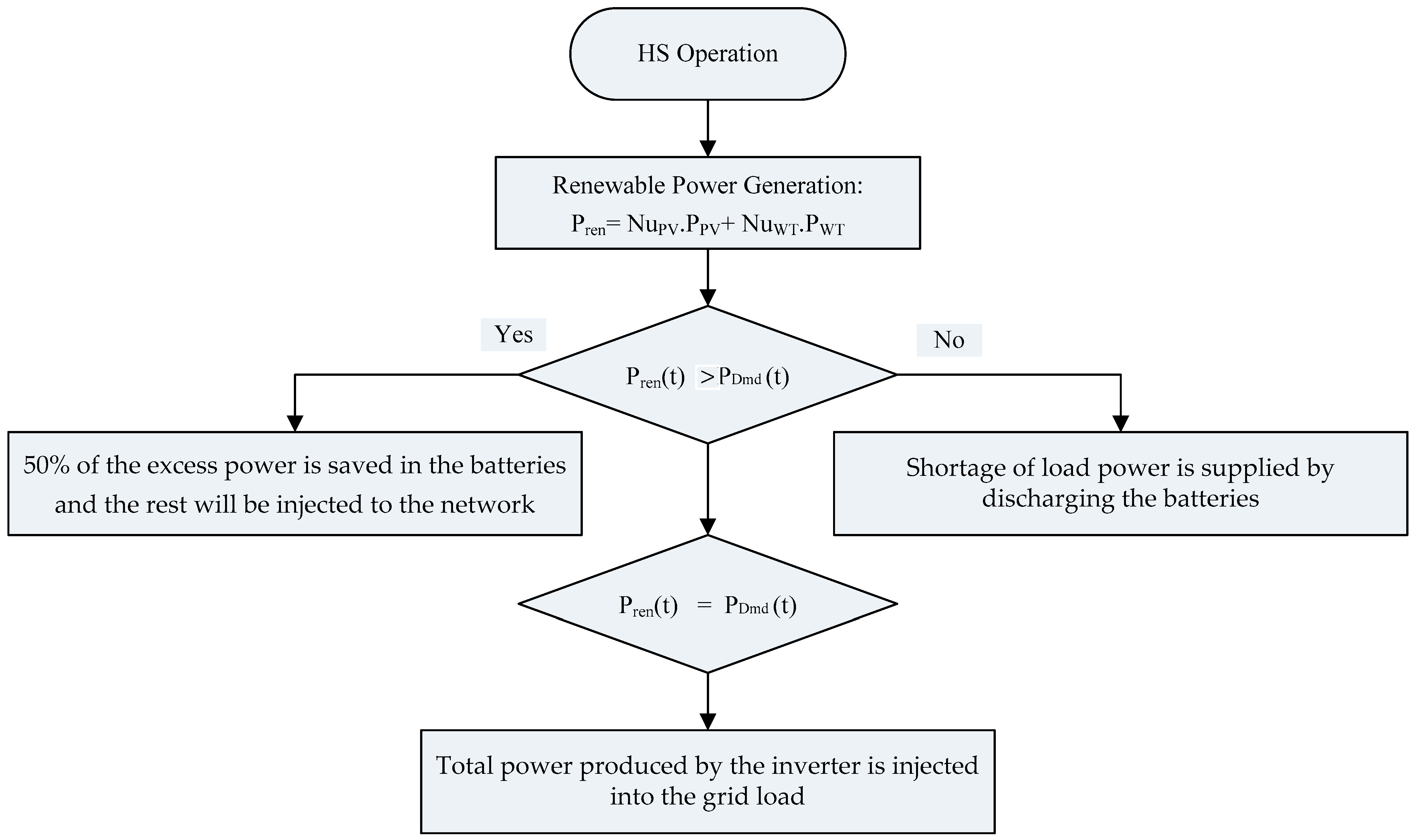
The studied HS included a photovoltaic system, wind turbines, and batteries. The batteries were used to compensate for the power fluctuations of renewable sources and create electrical scheduling and, thus, improve load reliability. The DC/DC converter was applied to boost the PV supply voltage, the AC/DC rectifier to convert wind power to DC power, and the DC/AC converter to convert DC power to AC power and transfer it to the distribution network. In Figure 1, different configurations of the HSs, including HPV/WT/Batt, PV/Batt, and WT/Batt, are shown.

3.1. Operation

The operation of the HS is described below:

• If the renewable generation is equal to the load, then the total power produced by the inverter is injected into the grid load.
• If the renewable generation is greater than the load, then 50% of the excess power is saved in the batteries and the rest will be injected into the network.
• If the renewable generation is less than the demand, then the shortage of load power is supplied by discharging the batteries.

The flowchart for the operation of the HS is presented in Figure 2.

3.2. Modeling

3.2.1. PV Model

The PV-produced power based on the irradiance and temperature is computed by [5,6]

$$P_{PV}(t)=P_{PV-No\min al}\times \frac{SI}{S{I}_{ref}}\times (1+{\rho }_T(Te{m}_c-Te{m}_{ref}))$$

(20)

where SI is radiation radiated to the PV panel (W/m²), $P_{PV-No\min al}$ denotes PV rated power, SI_ref is standard irradiance (1000 W/m²), ${\rho }_T$ is the coefficient of the PV temperature (−0.00371/°C), Tem_ref is the temperature of the PV in the standard condition and Tem_c denotes the temperature of the PV.

3.2.2. WT Model

The power of each WT based on the cut-in, nominal, and cut-out wind speed is computed as follows [5,6]:

$$P_{WT}^{}=\left\{\begin{array}{ll}0& ;v\le v_{ci},v_{}\ge v_{cout}\\ P_{WT-No\min al}\times {\left(\frac{v_{}-v_{cin}}{v_r-v_{cin}}\right)}^{}& ;v_{cin}\le v_{}\le v_r\\ P_{WT-No\min al}\stackrel{}{}& ;v_r\le v_{}\le v_{cout}\end{array}\right.$$

(21)

where v refers to the wind speed, v_cin and v_cout and v_r are the cut-in, cut-out and nominal wind speed, and P_WT-Nominal is the nominal power of each wind turbine. Wind data were collected at a 40 m wind-tower height; also, the height of the installation was 15 m. The wind speed in this condition was defined using $V_H=V_{Href}\times {\left.\left(\frac{\mathrm{H}}{H_{ref}}\right.\right)}^{\alpha }$, where $V_H$ is the wind speed with a height of H, $V_{Href}$ is the wind speed with height $H_{ref}$, and α is a value between 0.14 and 0.25 due to the ground roughness [15,16].

3.2.3. Batt Model

In hybrid energy systems, the role of the battery is to manage the charge and discharge of the power sources and compensate for their power fluctuations to create a continuous output power to supply the load and improve its reliability. The batteries’ charge and discharge modes in the HS are presented as follows [5,10]:

−

If renewable energy generation is more than the network load (the demand of a certain bus in the network), the battery is in charge mode (assuming that 50% of the additional power of the sources will be injected into the batteries and the rest will be transferred to the network to supply the specified load). The charge quantity of the battery at time t is computed by

$${\epsilon }_{Batt}(t)={\epsilon }_{Batt}(t-1)+\left[(N{u}_{PV}^{}\times P_{PV}^{}(t)+N{u}_{WT}^{}\times P_{WT}^{}(t))-\frac{P_{Dmd}^{}(t)}{E{f}_{Inv}}\right]\times \Delta t\times {\eta }_{ch}$$

(22)

where ${\epsilon }_{Batt}(t)$ and ${\epsilon }_{Batt}(t-1)$ refer to the battery charge values at time t and t − 1. $N{u}_{PV}^{}$ and $N{u}_{WT}^{}$ are the number of PVs and WTs. $P_{Dmd}^{}(t)$ is the load at time t and $E{f}_{Inv}$ is the inverter efficiency (here 90%).

−

If renewable generation is lower than the network load (The demand of a certain bus in the network), the battery is in discharged mode to provide the network demand. The efficiency of the battery is considered 90%. Therefore, the battery charge quantity at time t is calculated by [22,23]

$${\epsilon }_{Batt}(t)={\epsilon }_{Batt}(t-1)-\left[\frac{P_{Dmd}^{}(t)}{E{f}_{Inv}}-(N{u}_{PV}^{}\times P_{PV}^{}(t)+N{u}_{WT}^{}\times P_{WT}^{}(t))\right]\times \Delta t$$

(23)

4. Unscented Transformation for Stochastic Modeling

Uncertainties in the problem described in Equations (1)–(23) involve the production of solar and wind energy in addition to network consumption. In this study, the unscented transformation (UT) approach [27] was used to model the uncertain parameters. The UT does a good role of simulating decision making risks and uncertainty. It was developed on the principle that approximating a probability distribution is easier than estimating a result or transformation of any given nonlinear function. The core concept of the UT is to approximate the probability distribution function using a set of selected points called sigma points and accompanying weights. Metrics on the mean, variance, and other characteristics of mapping instances can be obtained by weighing these sigma points. The advantages of the UT include its ease of use and minimal sample size necessities. The size of the vector of inputs for uncertainty (U) in this approach is indicated by the parameter n, which was given an amount of three in this study. Furthermore, a probability of 2n + 1 was produced. Although there was no scenario reduction approach employed for this small set of options, the computation time was greatly reduced. The usage of the UT technique was to derive the mean and covariance values of the final results [27]. The steps to this approach are as follows:

−

Step 1: Choose 2n + 1 samples as the initial data for the parameters with uncertainty:

$$x_0={\mu }_x$$

(24)

$$x_s={\mu }_x\pm \sqrt{\frac{n}{1-W^0}\times {\sigma }_X},\forall s=1,2,\dots ,n$$

(25)

where $x\in R^n$ is the uncertain input vector, ${\mu }_x$ is the mean, ${\sigma }_x$ is the covariance of x, and W₀ is the weighted value of the mean quantity of x, which is equal to r.

−

Step 2: Compute each sample’s weightings:

$$W_0=W_0$$

(26)

$$W_s=\frac{1-W^0}{2n},\forall s=1,2,\dots ,n$$

(27)

$$W_{s+n}=\frac{1-W^0}{2n},\forall s+n=n+1,n+2,\dots ,2n$$

(28)

$${\displaystyle \sum _{s=1}^n{W}_s}=1$$

(29)

−

Step 3: Sample 2n + 1 indicates the nonlinear function for obtaining the outcome samples in accordance with Equation (30):

$$y_S=f(x_s)$$

(30)

where $y\in R^r$ is the uncertainty vector and has r elements.

−

Step 4: Calculate ${\mu }_y$ and ${\sigma }_y$ for variable θ.

$${\mu }_y={\displaystyle \sum _{s=1}^n{W}_s}{\theta }_s$$

(31)

$${\sigma }_y={\displaystyle \sum _{s=1}^n{W}_s(}{\theta }_s-{\mu }_y)-{({\theta }_s-{\mu }_y)}^T$$

(32)

5. Proposed Method

A new optimization algorithm, named the improved escaping-bird search algorithm (IEBSA), is applied to solve the scheduling of different configurations of the HS in distribution networks and, following its formulation, is presented.

5.1. Overview of the EBSA

Different types of living organisms have unique and advanced strategies to avoid predation. Apus Apus (swift) is one of the birds with a smooth and continuous flight that uses surface and vertical maneuvers to escape from predators. The prey bird uses diving behavior against the upward movement of the predator. These two maneuvers are shown in Figure 3. In Figure 3, the dashed line represents the path of the predator after being misled by the prey bird [26].

The situation of the artificial bird is presented as a vector that is modified by the flight of the bird. The maneuverability of the hypothetical bird i (MP_i) depends on the bird’s body area, wing beat rate, and the velocity, which is modeled as follows [26]:

$$M{P}_i=b_i{‖V_i‖}^{\beta }$$

(33)

$$‖V_i‖=\sqrt{{\displaystyle \sum _j{V}_{i,j}^2}}$$

(34)

where the vector of velocity V_i represents the current and last position differences related to the i-th bird.

The body coefficient (b_i) also presents the impact of body area (cost) in the form of the below equation [26]:

$$b_i=\frac{C_{\max }-C_i}{C_{\max }-C_{\min }+\epsilon }$$

(35)

where C_i is the cost of the agent i; C_max and C_min are the lowest and highest costs of the current population; and ε is a very small constant (provided to avoid the division by zero).

According to the maneuverability of the bird of prey (AB) and the bird of prey (EB), the escape rate (ER) is modeled as follows [26]:

$$ER=\frac{M{P}_{EB}}{M{P}_{AB}+M{P}_{EB}}$$

(36)

where MP_AB and MP_EB refer to the maneuverability of the predator bird and the prey bird.

The presented artificial flight is modeled as follows [26]:

$$X_{EB}=X_{EB}+r\times ER\times (Opp(X_{AB})-X_{EB})$$

(37)

where X_AB and X_EB represent the positions of the predator and prey birds, r refers to a random value created with a uniform distribution between 0 and 1, and ER represents the escape rate. The Opp(.) function expresses the vector’s opposite value in the search space and is presented by [26]:

$$Opp(X_{AB})=X_L+X_U-X_{AB}$$

(38)

In the condition of small ER, the prey bird executes the surface maneuver by changing the direction of its current position. This maneuver is modeled as follows [26]:

$$X_{EB}=X_L+R\otimes (X_U-X_L)$$

(39)

where X_L and X_U are the low and high values of the vector of variables, the sign $\otimes$ points to the element-wise product, and R denotes a random vector of values between 0 and 1.

In the process of evolution of the simulation, the flight towards the best experience of the preys (X_Gbest) is added; thus, the bird-of-prey maneuver is presented as follows [26]:

$$X_{AB}^{Candidate}=X_{AB}+r_1\times CR\times (X_{EB}-X_{AB})+r_2\times (X_{Gbest}-X_{EB})$$

(40)

where r₁ and r₂ are randomly produced in the range of 0 and 1, and the capturing rate (CR) is presented as follows [26]:

$$CR=1-ER$$

(41)

In the condition of a high ER value, the value of the capturing rate (CR) is zero and vice versa.

The steps of the EBSA based on the simulated maneuvers of the hypothetical birds of prey and predators are presented as follows:

Step (1) population generation of N artificial birds, randomly. The ith bird is produced as follows according to the lower and upper range of the design variables [26].

$$X_i=X_L+R\otimes (X_U-X_L)$$

(42)

Step (2) the amount of maneuvering power of each bird is calculated based on Equation (33) and the normalized cost values in Equation (34).

Step (3) the above main loop is executed until the convergence conditions are satisfied (as follows). For i, from 1 to N artificial birds, this operation should be performed.

▪

Calculate the $X_{AB}^{Candidate}$ cost.

▪

Under the condition that the cost of $X_{AB}^{Candidate}$ is less compared to X_AB, X_AB replaces it.

▪

Exit the loop after completing the number of evaluations of the cost function relative to the default value (NFE_max).

−

For EB based on either the surface maneuver or vertical maneuver, a candidate solution is generated. The transition between the described maneuvers is modeled as follows [26]:

$$X_{EB}^{Candidate}=\left\{\begin{array}{l}{X}_L+R\otimes (X_U-X_L)ifER<1/N\\ X_{EB}+r\times ER\times (Opp(X_{AB})-X_{EB})otherwise\end{array}\right.$$

(43)

-

Calculate the cost of $X_{AB}^{Candidate}$.

-

In the case of a lower cost of $X_{AB}^{Candidate}$ compared to X_EB, X_EB replaces it.

-

Exit from the main loop as soon as NFE reaches NFEmax.

-

Update X_Gbest.

-

Under the the condition that i = N and NFE < MNFE_max, go to Step three; otherwise, leave the loop and go to Step four.

Step (4) in this step, the updated X_best (optimal solution) is saved.

5.2. Overview of the IEBSA

In this study, the escape from the local optimum (EOLO) operator was used as a local search algorithm in the gradient-based optimizer to strengthen the algorithm’s discovery power and discover new areas in the search space. By strengthening the convergence behavior of the traditional EBSA algorithm, EOLO prevents its premature convergence [30,31]. In other words, it prevents the algorithm from getting stuck in the local optimum and improves the convergence performance of the algorithm.

EBSA generates solutions based on randomly generated solutions and the current best obtained solution. If a random number is smaller than the threshold number pr, the new position of x_EOLO is defined as follows [30,31]:

$$\begin{array}{ll}{x}_{EOLO}& =x_i+f_1(u_1\times x_{best}-u_2\times x_k)+f_2\phi (x_{2R}-x_{1R})\\ & +u_2\phi (x_{r1}-x_{r2})/2\end{array}$$

(44)

If the random number is greater than the limit of pr, then the new position of x_EOLO is presented as follows [30,31]:

$$\begin{array}{ll}{x}_{EOLO}& =x_{best}+f_1(u_1\times X_{best}-u_2\times x_k)+f_2\phi (u_3(x_{2R}-x_{1R}))\\ & +u_2(x_{r1}-x_{r2})/2\end{array}$$

(45)

where x_i represents the current position of individual i, x_best is the current best solution, f₁ and f₂ are random numbers with a uniform distribution in the range [−1, 1], and x_r1 and x_r2 are random solutions selected from the population. x_1R and x_2R represent stochastic solutions in the lower and upper bounds. Also, the random variables u₁, u₂ and u₃ are defined by

$$\begin{array}{l}{u}_1=L_1\times 2\times rand+(1-L_1)\\ u_2=L_1\times rand+(1-L_1)\\ u_3=L_1\times rand+(1-L_1)\end{array}$$

(46)

where L₁ represents the binary parameter, rand refers to a random number in the range [0, 1].

To balance the diversity in the search process, the parameter φ is obtained as follows [30,31]:

$$\phi =2\times rand\times \alpha -\alpha$$

(47)

$$\alpha =\left|\beta \times \sin (\frac{3\pi }{2}+\sin (\beta \times \frac{3\pi }{2}))\right|$$

(48)

$$\beta ={\beta }_{\min }+({\beta }_{\max }-{\beta }_{\min })\times {(1-{(\frac{iter}{\max Iter})}^3)}^2$$

(49)

where b_min and b_max are the lower and upper limits of the step-size parameter, which were selected as 0.2 and 1.2, respectively.

The solution x_k is defined as follows:

$$x_k=L_2\times x_{r3}+(1-L_2)\times x_{rand}$$

(50)

where x_rand represents the random solution, x_r3 represents a random selection from the population set, and L₂ represents a binary parameter.

Therefore, based on the presented EOLO, it strengthens the local discovery power of the algorithm and adds to its ability to reach the global solution faster.

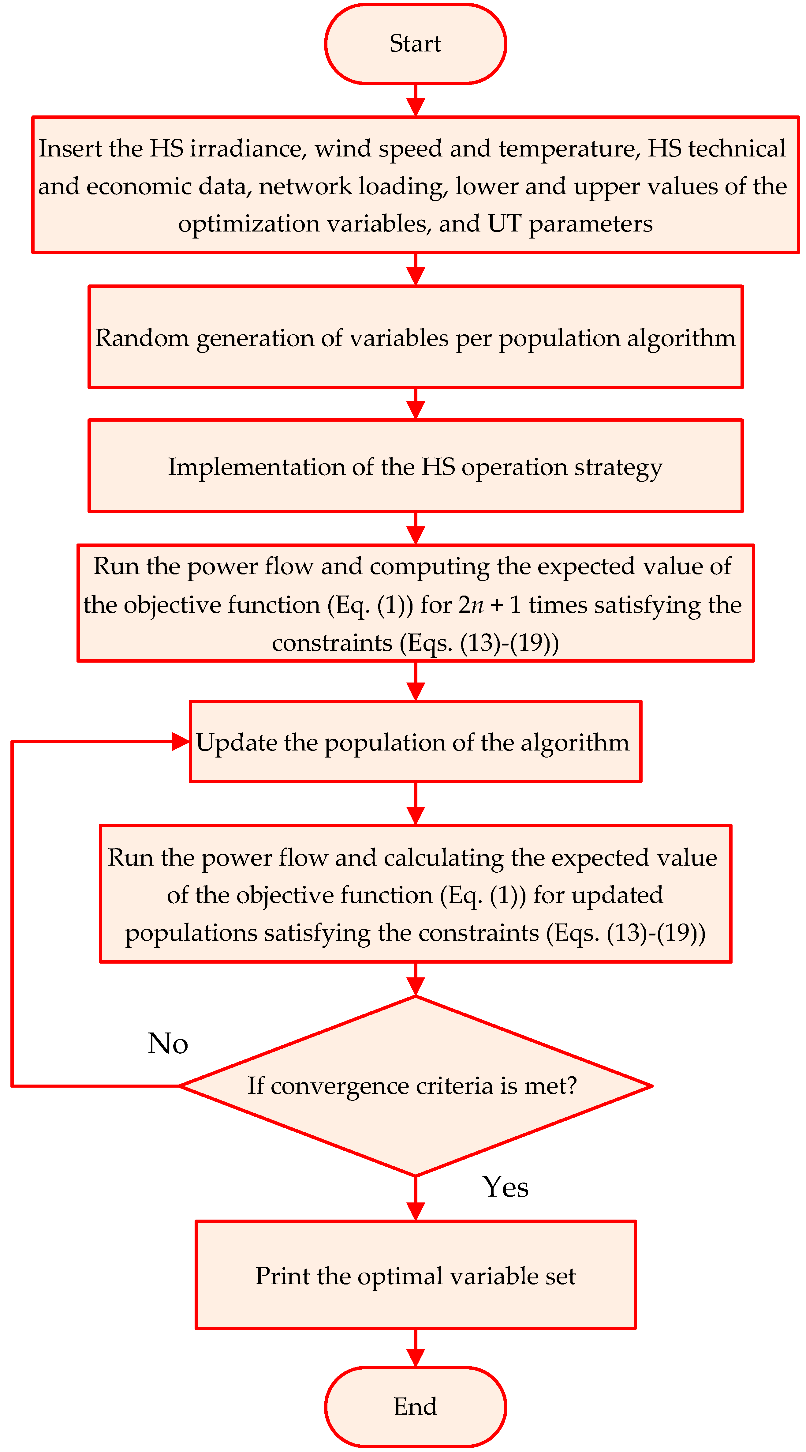
5.3. The Implementation of IEBSA Based on the UT

The following are the deterministic implementation steps of the IEBSA integrated with the UT approach presented in Section 4, used to schedule the HS energy system:

Step 1: Enter the data. The data include load and network line information, economic information about the cost of solar, wind, and battery storage, load demand information, solar radiation, the rated size, and system equipment efficiency. Also, the algorithm’s general parameters like population size, maximum iterations, and repetition were selected as 50, 50, and 25, respectively. The general parameters of the algorithms are determined based on the user experience and repeated runs in achieving a different solution. Moreover, in this step, UT parameters including the number of uncertain parameters and the PDF of the uncertain parameters are initiated.

Step 2: Add the population as a decision factor set, which also includes the amount of PVs and batteries as well as where the HS energy system will be installed in the network. In the search space, the main population is generated at random. The variable set is presented first.

Step 3: Operating the HS. The HS operating plan is put into practice in this part.

Step 4: Calculate the expected value of the OF (Equation (1)) using the UT stochastic method and research the constraint (Equations (13)–(19)) of the challenge. In the UT method, for n random variables, the problem is solved 2n + 1 times. For each solution, the expected value of the OF is calculated 2n + 1 times by the use of UT. At this point, the restrictions connected to the HS system components and network optimum functioning are disclosed to the OF (Equation (1)). The best variable set with the lowest expected value of the OF is chosen at this stage.

Step 5: Update the algorithm population and choose variables at random in accordance with the IEBSA.

Step 6: Determine the problem constraint (Equations (13)–(19)) and compute the expected value of the OF (Equation (1)) for the IEBSA’s revised population. The related variable set is regarded as the best set if the value of the expected value of the OF (Equation (1)) acquired in Step 6 is superior than the expected value of the OF (Equation (1)) obtained in Step 4.

Step 7: Were the convergence requirements—obtaining the lowest expected value of the OF (Equation (1)) and using the most iterations—met? If so, go to Step 8; otherwise, go to Step 5.

Step 8: Stop the algorithm and record the outcomes (using the HS system’s ideal installation location and size as decision variables).

A flowchart of the implementation of the IEBSA to solve the scheduling problem is depicted in Figure 4.

6. Results and Discussion

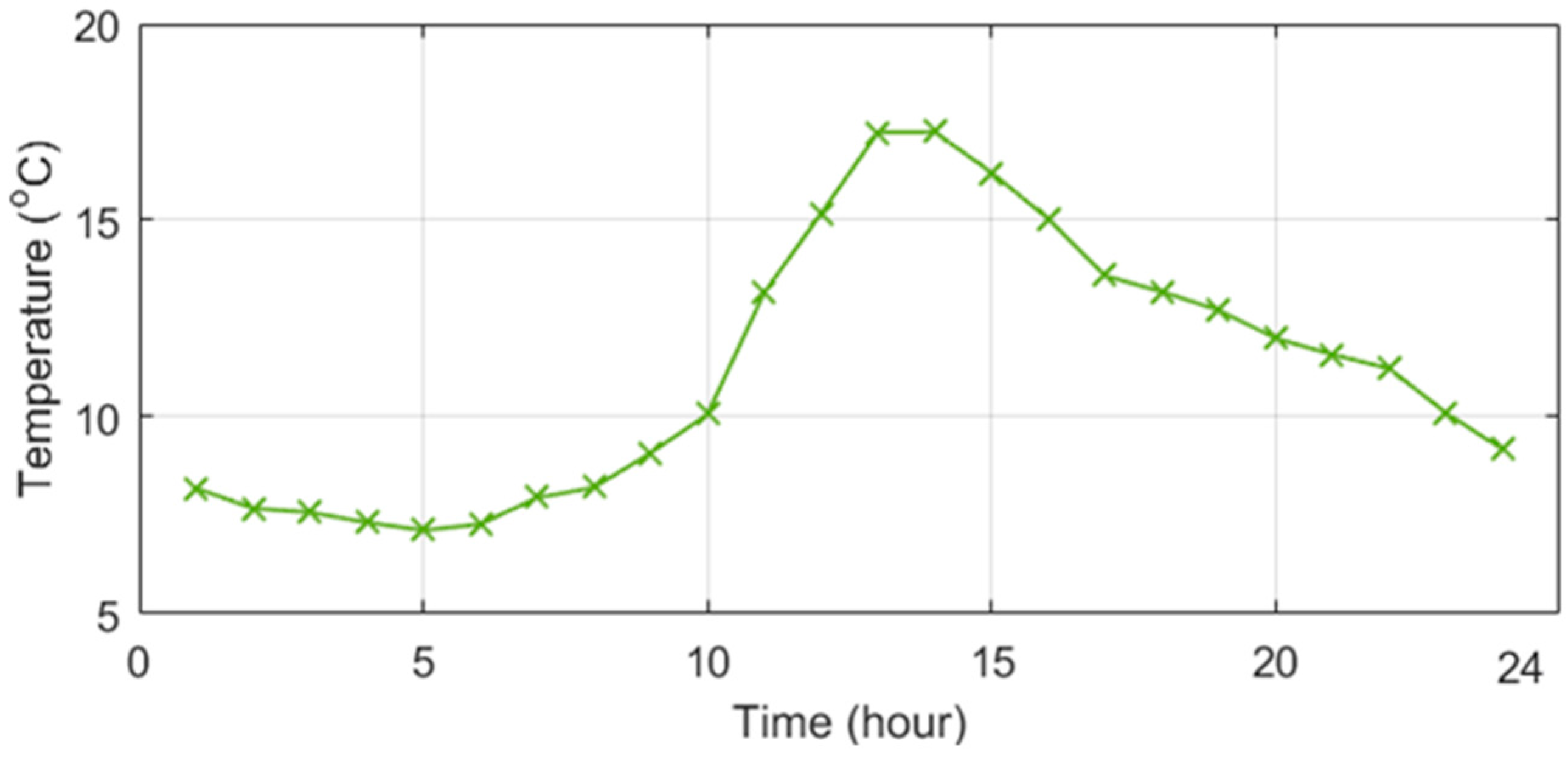
6.1. System Data

The HPV/WT/Batt system’s scheduling results in the 33-bus distribution network are shown in order to observe if the system minimizes energy losses, voltage variations, and ENS, as well as the cost of HS energy production. Figure 5 shows the network diagram for the 33-bus network. The demand and branch data for the 33-bus network were taken from [32]. The overall load in the 33-bus network was 3.72 MW and 2.3 MVAr. The suggested technique was implemented in this research using the MATLAB environment (R2015b) and a personal computer running Windows 7, with a Core i7 processor running at 3.1 GHz, 8 GB of RAM, and a 1 T hard drive. In this study, the optimal value of the weight coefficients of the objective functions, calculated using Equation (1), was determined using the IEBSA. In other words, the lower limit of each coefficient was equal to 0 and the maximum limit of each coefficient was equal to 1. Also, the steps considered for the changes of the weight coefficients were included, with a value of 0.1. The basic simulation was performed using the proposed IEBSA 20 times, and as a result, the values of the weight coefficients of each function were extracted based on the best result. The values of the weight coefficients ${\psi }_1$, ${\psi }_2$, ${\psi }_3$, and ${\psi }_4$ (in Equation (1)) were calculated as 0.29, 0.22, 0.28, and 0.21, respectively.

The PV module, named the KC200GT model, was selected with a peak power voltage, peak power current and peak power equal to 26.3 V, 7.61 A and 200 W, respectively. The open-circuit voltage, and short-circuit current were 32.9 V and 8.21 A, respectively. In this study, the PV array with a unit power of 1 kW was formed by the combination of the modules. The series and shunt resistances were 2 and 100 Ω, respectively. The meteorological data were taken from ref. [33]. The irradiance, wind speed, and temperature data were taken from ref. [34] (located in latitude 37°24′ and longitude 55°15′) for 1 January 2019.

The profiles of irradiance, wind speed, and temperature are depicted in Figure 6, Figure 7 and Figure 8, respectively, for a 24 h period. Also, the network loading was taken from ref. [35] and depicted in Figure 9. The HS component’s technical and economic data are also given in

Table 2. Technical and economic data of photovoltaic array [23,24].

Parameters	Values
Nominal power	1 kW
Lifetime	20 years
Reference irradiance	1000 W/m2
Reference temperature	25 °C
Temperature coefficient	−0.0037
Capital cost	USD 2000
Operation and maintenance cost	33 USD/year

,

Table 3. Technical and economic data of wind turbine [23,24].

Parameters	Values
Nominal power	1 kW
lifetime	20 years
Vcin	3 m/s
Vcout	20 m/s
Vr	13 m/s
Capital cost	USD 3200
Operation and maintenance cost	100 USD/year

and

Table 4. Technical and economic data of battery [23,24].

Parameters	Values
Maximum capacity	1 kAh
Minimum capacity	0.2 kAh
Charge efficiency	0.9
Discharge efficiency	0.9
Depth of discharge	0.8
lifetime	5 years
Capital cost	USD 100
Operation and maintenance cost	5 USD/year

.

6.2. Results of Deterministic Scheduling (without Uncertainty)

The results of HS scheduling incorporated with battery energy storage are presented for the different configurations in the 33-bus distribution network for minimizing the energy losses, voltage deviations, and energy not supplied, as well as the HS energy generation cost using the IEBSA. In other words, the best configuration for a HS consisting of renewable energy sources and battery storage to solve the planning problem, with the most favorable effect on the distribution network, has been determined.

The convergence process obtained from solving the scheduling problem, using the IEBSA for different configurations of the HS, is depicted in Figure 10. The performance of the proposed algorithm in planning the configuration of the HPV/WT/Batt system in the network, with a high convergence speed and low convergence tolerance when achieving the global optimal solution, is clear. Examining the convergence curves shows the better performance of the HPV/WT/Batt configuration in network scheduling, with it achieving a lower OF value.

The results of HS scheduling in the 33-bus network using the IEBSA, considering different configurations, are given in

Table 5. The scheduling results of HS in the 33-bus network using the IEBSA, considering different configurations.

Item/Value	Base Network	With HPV/WT/Batt	With PV/Batt	With WT/Batt
Number of WTs	--	488	606	--
Number of PVs	--	134	--	589
Number of Batts	--	648	11	986
Installation Location (@Bus)	--	@30	@12	@10
Annual Energy Losses (kWh)	1436.17	960.88	1168.66	889.54
Energy Not Supplied (MWh)	9.41	4.37	8.22	6.51
Voltage Deviation (p.u)	0.7602	0.2811	0.5361	0.2824
Energy System cost (USD)	--	1,455,800	455,050	1,628,756
Objective Function	--	0.5628	0.8386	0.6309

. The OF values for HS scheduling in the 33-bus network, using IEBSA considering configurations such as HPV/WT/Batt, PV/Batt, and WT/Batt, were calculated as 0.5628, 0.8386, and 0.6309, respectively, which elucidates the superior performance of the system using PV and WT sources along with battery storage as the optimal HS configuration. The IEBSA in the HPV/WT/Batt system scheduling installed 134 photovoltaic panels, 488 wind turbines, and 648 batteries in bus 4 of the 33-bus network. The results demonstrated that the values of energy losses were reduced from 1436.17 kWh to 960.88 kWh, the energy not supplied declined from 9.41 MWh to 4.37 MWh, the voltage deviations decreased from 0.7602 p.u to 0.2811 p.u, and the annual cost of the HS was USD 1,455,800 for the optimal HPV/WT/Batt configuration. Comparing the results obtained from the HPV/WT/Batt system with other configurations shows that this configuration obtained lower values of energy losses, unsupplied energy, voltage deviations, and energy costs. In addition, it can be seen that the weakest ability to improve each of the objectives of the study was achieved by the PV/Batt configuration; in other words, photovoltaic arrays are not able to enhance the network characteristics in addition to battery storage like other configurations, and it is clear that the improvement in subscriber reliability using this configuration is weak compared to other configurations.

In Figure 11, the power values of the battery bank over 24 h show that the battery storage system with a charging and discharging capability injected schedulable power into the distribution network, and this significantly improved each of the objectives. Also, the reserve power management significantly improved the reliability of the network subscribers from 9.41 MWh to 4.37 MWh (53.56%). It can be seen that the PV/Batt configuration has the lowest level of storage participation, WT/Batt configuration has the highest level of storage contribution and the optimal HPV/WT/Batt configuration has an optimal level of storage.

In Figure 12, the changes in the production power of the photovoltaic array are plotted for the HPV/WT/Batt and PV/Batt systems, in which the maximum power production is from 10:00 to 15:00 h. It is clear that the level of PV power production in the PV/Batt configuration was higher than the HPV/WT/Batt configuration because in the PV/Batt configuration, the photovoltaic sources alone produced power.

The changes in wind power generation for the HPV/WT/Batt and WT/Batt configurations are presented in Figure 13. The WT power generation in the WT/Batt configuration was higher than the WT/Batt system because the only sources of production in this configuration were wind turbines.

Figure 14, Figure 15 and Figure 16 show the change curves of energy losses the energy not supplied by the network subscribers, the voltage deviations of the 33-bus network for the state without the HS, and the different configurations of the HS. The results show that with the optimal scheduling of the different HS configurations, the power loss was reduced in all hours compared to the base network. According to Figure 14, the HPV/WT/Batt configuration obtained lower losses in the most hours compared to the other configurations. Figure 14 shows the weakest performance of the PV/Batt system in reducing losses from 18:00 to 24:00 h.

Based on Figure 15, the optimal HPV/WT/Batt configuration improved the reliability across all hours more than the other configurations. In other words, it obtained the lowest ENS across all hours, which was due to the overlap of the photovoltaic and wind sources with each other, as well as reserve-power management. In addition, the weakest reliability improvement performance was related to the PV/Batt configuration.

Based on Figure 16, the lowest voltage deviations were related to the HPV/WT/Batt and WT/Batt configurations. According to Table 5, the voltage deviation values using the HPV/WT/Batt and WT/Batt configurations were measured as 0.2811 p.u and 0.2824 p.u, respectively; therefore, the HPV/WT/Batt system performance is a little better in improving the voltage profile. However, both configurations performed well in improving the voltage profile of the 33-bus network.

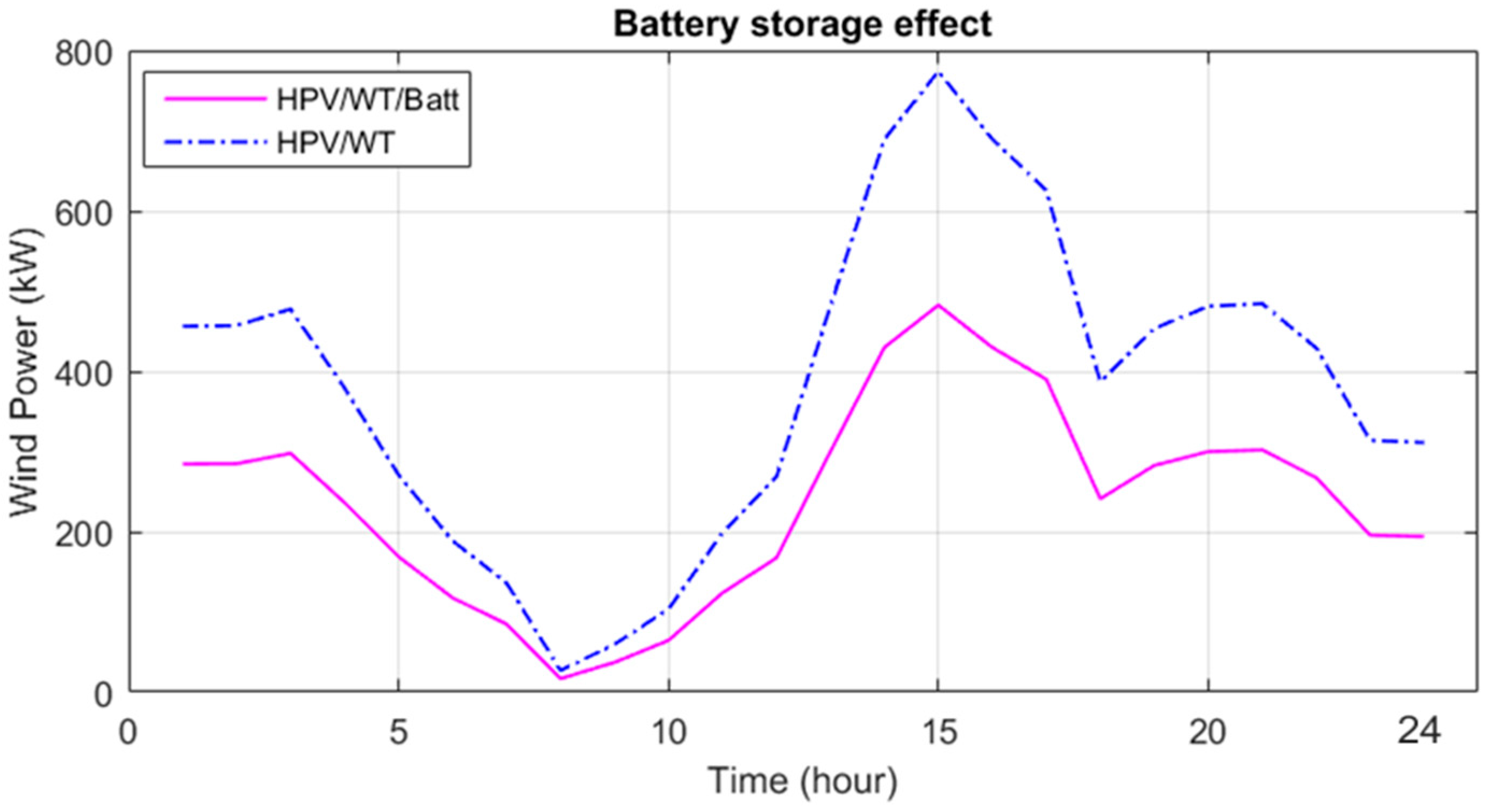
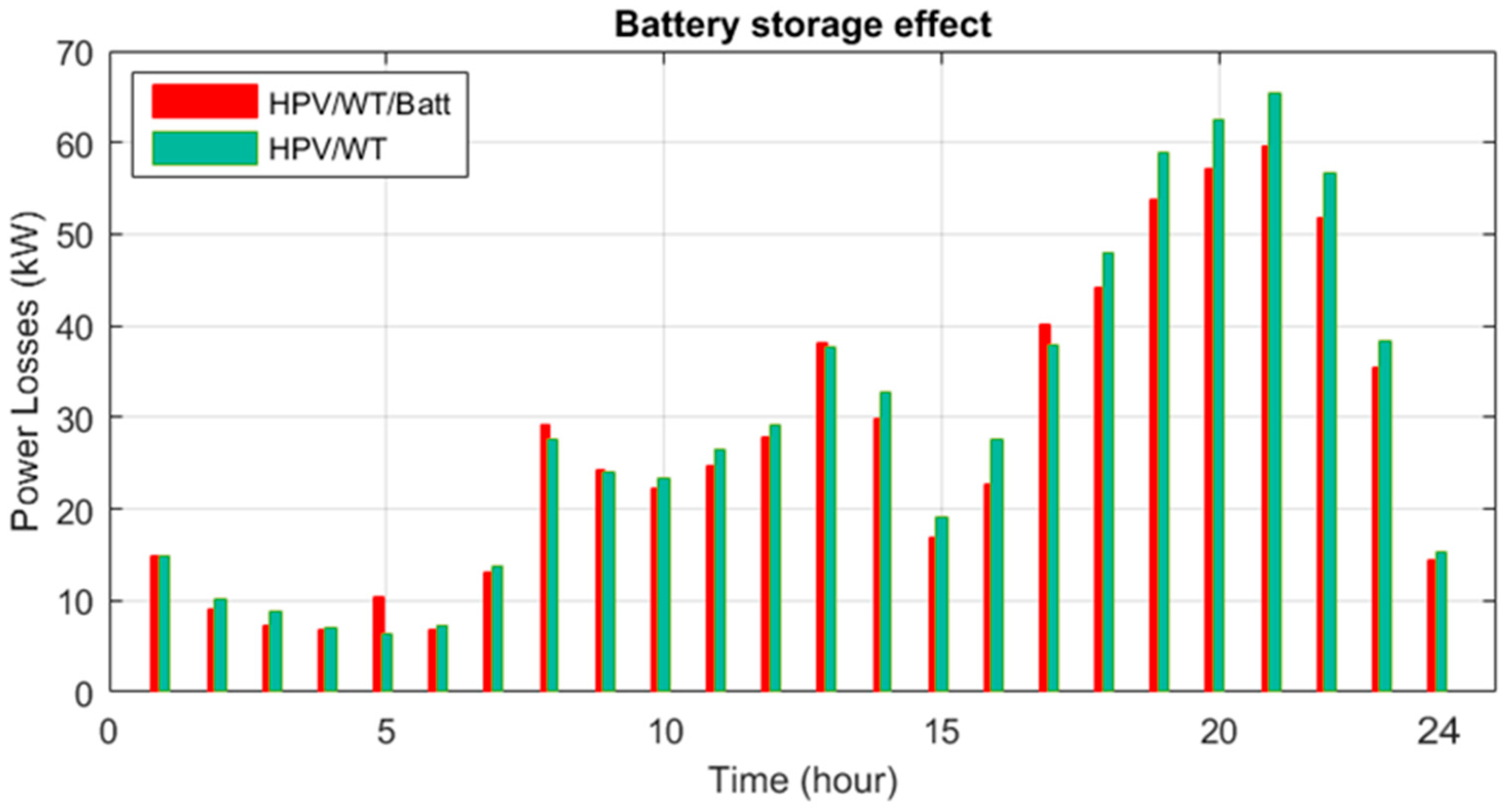
6.2.1. Results of the Battery Storage Effect

The role of the battery storage system in the HPV/WT energy system is to create an electrical schedule and programmable power injection according to the needs of the network over 24 h of the study. The battery storage effect in the HS system’s scheduling was evaluated in the distribution network. The scheduling results with and without battery storage in the 33-bus network, using the IEBSA, are presented in

Table 6. The scheduling results of the HPV/WT system with and without storage in a 33-bus network using the IEBSA.

Item/Value	Base Network	With Battery Storage	Without Battery Storage
Number of WTs	--	488	783
Number of PVs	--	134	229
Number of Batts	--	648	--
Installation Location (@Bus)	--	@30	@10
Annual Energy Losses (kWh)	1436.17	960.88	985.32
Energy Not Supplied (MWh)	9.41	4.37	4.87
Voltage Deviation (p.u)	0.7602	0.2811	0.2812
Energy System cost (USD)	--	1,455,800	2,226,760
Objective Function	--	0.5628	0.6130

. It can be seen that in planning without battery storage, renewable resources are forced to produce more power; thus, the cost of unscheduled power production increased greatly (increase from USD 1,455,800to USD 2,226,760 (52.68% increase)). On the other hand, the energy loss increased by 2.54%, reliability weakened by 11.44%, and the voltage deviations did not change. Therefore, the results confirmed that the storage device significantly reduced energy production costs, as well as reducing losses and improving network reliability.

The power production curves for the photovoltaic and wind turbines are shown in Figure 17 and Figure 18, from which it is clear that the production of these resources increased significantly without considering the battery storage. In other words, the non-schedulable production of renewable resources had to increase to satisfy various objectives.

The curves for energy loss and ENS without and with the battery storage for the HS are shown in Figure 19 and Figure 20. It can be seen that the power loss, as well as the ENS, when using battery storage for most of the hours, was lower than when not using it in the HS scheduling in the network.

6.2.2. The IEBSA Superiority

In this section, the proposed scheduling-based IEBSA performance was compared with the conventional EBSA, PSO, and a gazelle optimization algorithm (GOA). The set parameters of different algorithms are given in

Table A1. Set parameters of the different algorithms [26,28,29].

Parameters	EBSA	PSO	GOA
Constriction factor χ	--	0.80	--
Acceleration control coefficient c1	--	2.00	--
Acceleration control coefficient c2	--	2.00	--
s	--	--	[0, 1]
PSRs	--	--	0.34
Population	50	50	50
Maximum iteration	50	50	50
Repetition	25	25	25

in Appendix A. The convergence curve obtained from different methods in Figure 21 shows that the IEBSA was capable of obtaining a lower OF quantity, in terms of higher convergence speed and accuracy, and a lower convergence tolerance than other methods. It can be seen that the conventional EBSA has premature convergence and is stuck in the local optimum, so its improvement using the escape operator from the local optimal (EOLO) method improved its convergence process (in the form of IEBSA).

The scheduling results using different algorithms are presented in

Table 7. The scheduling results of the HPV/WT/Batt system in a 33-bus network using different algorithms.

Item/Value	IEBSA	EBSA	PSO	GOA
Number of WTs	488	572	478	536
Number of PVs	134	93	155	197
Number of Batts	648	1690	2505	886
Installation Location (@Bus)	@30	@10	@30	@10
Annual Energy Losses (kWh)	960.88	894.24	960.56	906.15
Energy Not Supplied (MWh)	4.37	6.35	4.36	6.30
Voltage Deviation (p.u)	0.2811	0.2724	0.2812	0.2748
Energy System Cost (USD)	1,455,800	1,656,756	1,464,637	1,641,228
Objective Function	0.5628	0.6206	0.5658	0.6197

. According to Table 2, the IEBSA achieved a smaller OF quantity compared with the conventional EBSA, PSO, and GOA algorithms. Also, the energy losses were computed as 960.88 kW, 894.24 kW, 960.56 kW, and 906.15 kW; the ENS values obtained were 4.37 MWh, 6.35 MWh, 4.36 MWh, and 6.30 MWh; the voltage deviation values were 0.2811 p.u, 0.2724 p.u, 0.2812 p.u and 0.2748 p.u; and the HS costs were calculated as USD 1,455,800, USD 1,656,756, USD 1,464,637 and USD 1,641,228 using the IEBSA, conventional EBSA, PSO, and GOA algorithms, respectively. This, along with the results from Table 7 and the obtained statistical analysis results presented in

Table 8. The performance of algorithms in HPV/WT/Batt scheduling in 33-bus network using statistic analysis.

Method	Best	Mean	Worst	STD
IEBSA	0.5628	0.5809	0.5973	0.0531
EBSA	0.6206	0.6395	0.6524	0.0994
PSO	0.5658	0.5910	0.6037	0.06703
GOA	0.6197	0.6284	0.6320	0.0746

with better criteria, prove the superior performance of the proposed methodology based-IESBA.

6.2.3. Validation of the IEBSA Deterministic Results with a Previous Study

The results of the IEBSA in the HPV/WT/Batt system scheduling in the 33-bus network were compared with ref. [33], which studied the scheduling of the a HPV/WT/Batt energy system in the 33-bus distribution network, to minimize the losses and voltage deviations, using a two-objective optimization approach via an improved crow search algorithm. The drawback of ref. In [33], the HS generation cost and reliability of the OF is not considered for solving the scheduling problem. The comparison results in

Table 9. Comparison of the IEBSA performance with ICSA [33].

Item/Value	IEBSA	[33]
Number of WTs	488	672
Number of PVs	134	802
Number of Batts	648	2889
Installation Location (@Bus)	@30	@30
Annual Energy Losses Reduction (%)	33.09	43.80
Energy Not Supplied (MWh)	4.37	--
Voltage Deviation Reduction (%)	63.02	38.51
Energy System cost (USD)	1,455,800	2,438,870

confirm the superior capability of the proposed methodology based-IEBSA to obtain a greater reduction in the percentage of power losses, voltage deviations, and HS energy generation costs, compared with ref. [33].

6.3. Results of Stochastic Scheduling (with Uncertainty)

The results of the HS stochastic scheduling with battery energy storage, considering the uncertainties of the renewable resources generation and the network load, are given for the optimal HPV/WT/Batt configuration in the 33-bus distribution network to minimize the energy losses, voltage deviations, and energy not supplied, as well as the HS energy generation cost, using the IEBSA and UT approach.

In order to use the UT method for modeling the uncertainties of photovoltaic and wind energy resources, as well as the load demand in the proposed optimization problem, the expected value of the objective function was calculated during the optimization process. In the first step, the covariance matrix was constructed using the standard deviation and correlation values as the symmetrical and unsymmetrical elements of the covariance matrix, respectively [27]. The mean value of the uncertain parameters made the μ_x vector in (24). By having covariance matrix_, μ_x and the weighing factor for the uncertain parameters from (15), (16), (17), 2n + 1 sample vectors were generated from (26)–(29). Considering the 2n + 1 vectors, the objective function was calculated 2n + 1 times as shown in (30). Finally, the 2n + 1 values of cost function were aggregated to make a unit expected value for the cost objective function as (32).

The capacity of photovoltaic and battery resources as well as storage capacity and the different objective values for the deterministic models (without uncertainty) and stochastic model (with uncertainty based on the UT approach) are presented in

Table 10. Comparison of the results of stochastic and deterministic scheduling of the HPV/WT/Batt system in a 33-bus network using the IEBSA.

Item/Value	Deterministic	Stochastic
Number of WTs	488	497
Number of PVs	134	131
Number of Batts	648	724
Installation Location (@Bus)	@30	@30
Annual Energy Losses (kWh)	960.88 (33.09%)	982.38 (31.59%)
Energy Not Supplied (MWh)	4.37 (53.56%)	4.59 (51.22%)
Voltage Deviation (p.u)	0.2811 (63.02%)	0.2873 (62.56%)
Energy System Cost (USD)	1,455,800	1,483,659
Objective Function	0.5628	0.5974

. According to this table, in the HS stochastic scheduling, different objectives such as power losses, voltage deviations, the ENS and the energy cost of the optimal HPV/WT/Batt combination increased (weakened) by 2.23%, 5.03%, 2.20%, and 1.91%, respectively, (Figure 22) compared to the deterministic scheduling. The results showed that due to the uncertainty of the production capacity of renewable resources and network load, the cost of energy injected into the network by the HPV/WT/Batt increased. Therefore, until the power fluctuations of renewable resources and load demand are not compensated compared to scheduling with the deterministic model, a higher level of storage should be used in the stochastic planning model than in the deterministic model.

7. Conclusions

In this study, the stochastic scheduling of various configurations of the hybrid energy systems, including HPV/WT/Batt, PV/Batt, and WT/Batt energy systems, in the distribution network was presented to minimize the energy losses, voltage deviations, HS cost, and also the ENS, utilizing the UT. The IEBSA was used to find the installation location of the HS and also the number of PVs, wind turbines, and batteries. The scheduling approach based-IEBSA was optimized using the weighted coefficients method satisfying the HS and network operating constraints. The research findings are presented below:

−

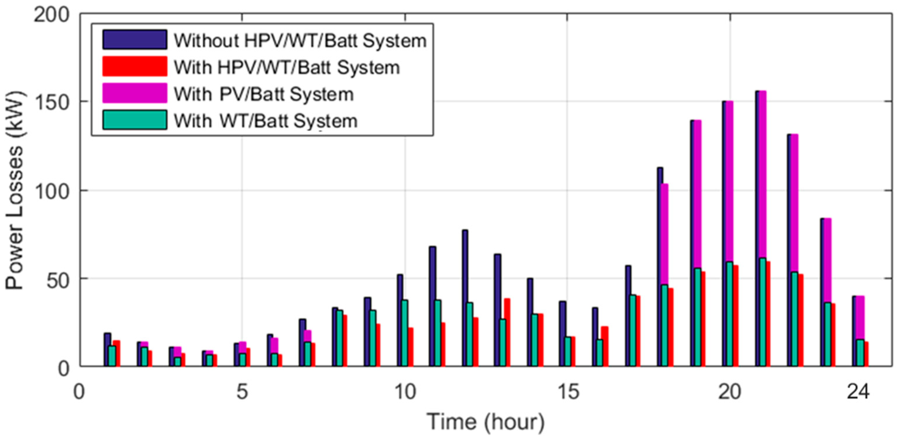
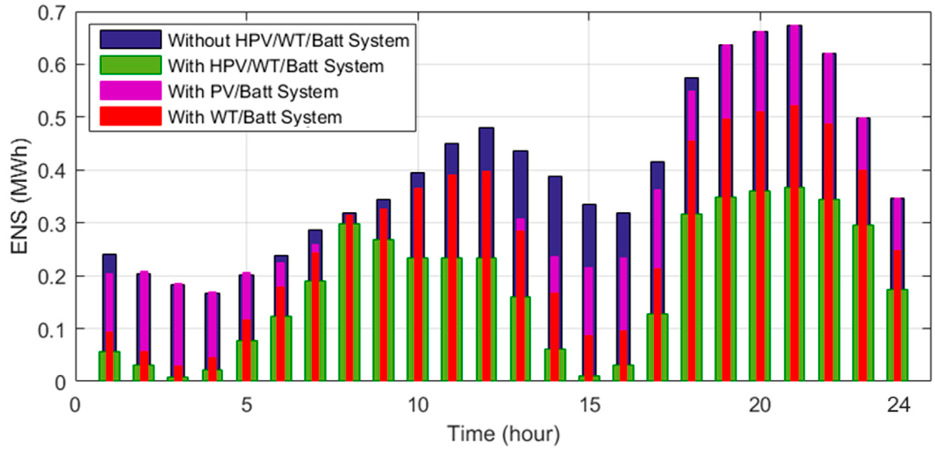
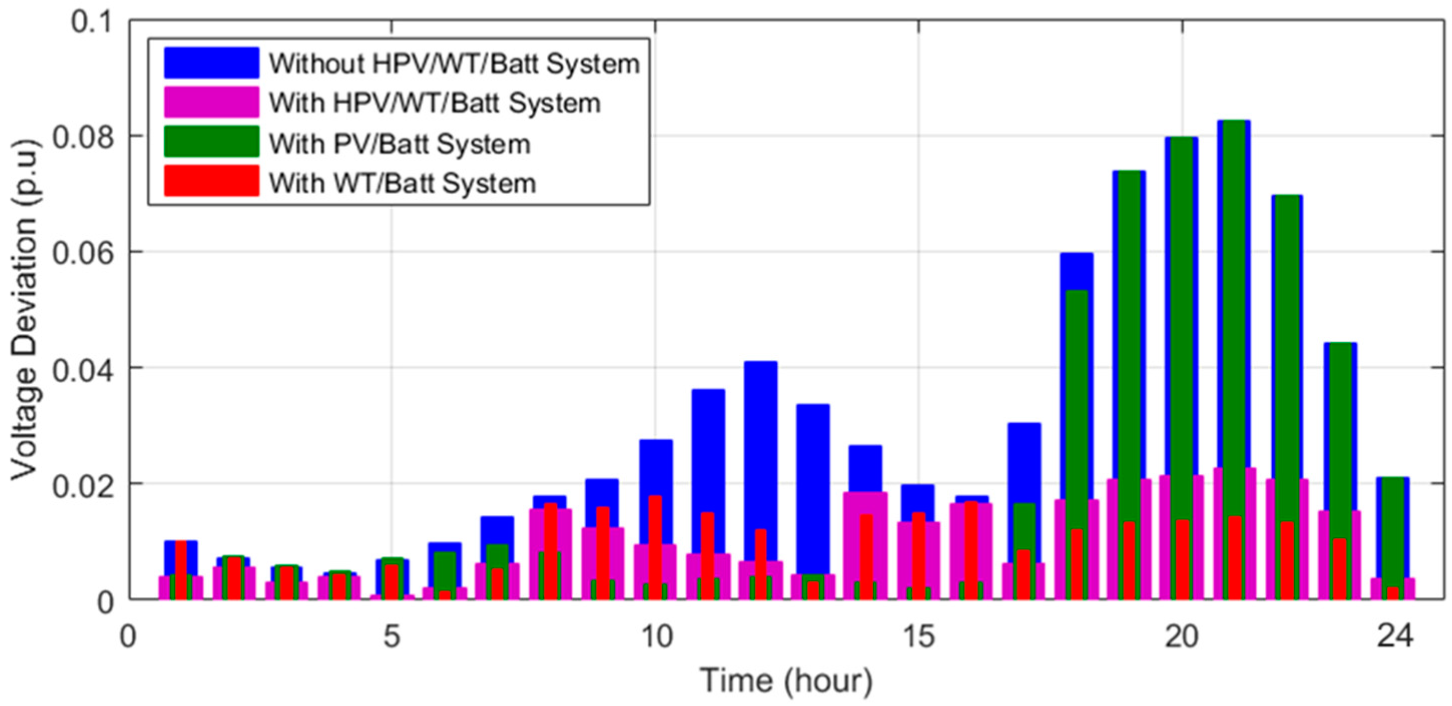
The results showed that the HPV/WT/Batt configuration obtained better objectives than the other combinations such as the lowest values of energy losses, voltage deviations, HS costs, and also the highest reliability levels compared to the other system configurations. The energy losses reduced from 1436.17 kWh to 960.88 kWh, ENS declined from 9.41 MWh to 4.37 MWh, voltage deviations decreased from 0.7602 p.u to 0.2811 p.u and the HS cost obtained was USD 1,455,800. Also, the results showed that the PV/Batt was the weakest configuration in achieving different objectives improvement, especially in hours of network peak load.

−

The results showed that integrating the battery storage with the HPV/WT system scheduling decreases the energy losses, ENS, voltage deviations, and also HPV/WT/Batt cost by 0.26%, 10.26%, 0.03%, and 34.62%, respectively, compared to the absence of the storage system.

−

The comparison of the IEBSA results with the conventional EBSA, PSO, and GOA algorithms show its superiority in overcoming the premature convergence based on the escape operator from the local optimal and achieving lower values for different objectives. Also, the superior performance of the proposed methodology-based IEBSA was proved when compared to the previous study of ref. [33].

−

Results of the stochastic scheduling, based on the UT approach, demonstrated that the energy losses, voltage deviations, and the ENS, and the HPV/WT/Batt energy cost increased due to the consideration of the uncertainties. The low number of sampling points makes this approach an efficient uncertainty model.

−

The robust scheduling of the HPV/WT energy system, using battery hydrogen multi-storage, to improve reliability and power quality indices in a distribution network is suggested for future research.

References

1. Zhang, X.; Wang, Y.; Yuan, X.; Shen, Y.; Lu, Z.; Wang, Z. Adaptive dynamic surface control with disturbance observers for battery/supercapacitor-based hybrid energy sources in electric vehicles. IEEE Trans. Transp. Electrif. 2022, 99, 1–11. [Google Scholar] [CrossRef]
2. Al-Najjar, H.; El-Khozondar, H.J.; Pfeifer, C.; Al Afif, R. Hybrid grid-tie electrification analysis of bio-shared renewable energy systems for domestic application. Sustain. Cities Soc. 2022, 77, 103538. [Google Scholar] [CrossRef]
3. Jiang, J.; Zhang, L.; Wen, X.; Valipour, E.; Nojavan, S. Risk-based performance of power-to-gas storage technology integrated with energy hub system regarding downside risk constrained approach. Int. J. Hydrogen Energy 2022, 47, 39429–39442. [Google Scholar] [CrossRef]
4. Dini, A.; Pirouzi, S.; Norouzi, M.; Lehtonen, M. Grid-connected energy hubs in the coordinated multi-energy management based on day-ahead market framework. Energy 2019, 188, 116055. [Google Scholar] [CrossRef]
5. Zhang, X.; Lu, Z.; Yuan, X.; Wang, Y.; Shen, X. L2-gain adaptive robust control for hybrid energy storage system in electric vehicles. IEEE Trans. Power Electron. 2020, 36, 7319–7332. [Google Scholar] [CrossRef]
6. Kilic, M.; Altun, A.F. Dynamic modelling and multi-objective optimization of off-grid hybrid energy systems by using battery or hydrogen storage for different climates. Int. J. Hydrogen Energy 2023, 48, 22834–22854. [Google Scholar] [CrossRef]
7. Wang, Z.; Zhao, D.; Guan, Y. Flexible-constrained time-variant hybrid reliability-based design optimization. Struct. Multidiscip. Optim. 2023, 66, 89. [Google Scholar] [CrossRef]
8. Nowdeh, S.A.; Davoudkhani, I.F.; Moghaddam, M.H.; Najmi, E.S.; Abdelaziz, A.Y.; Ahmadi, A.; Razavi, S.E.; Gandoman, F.H. Fuzzy multi-objective placement of renewable energy sources in distribution system with objective of loss reduction and reliability improvement using a novel hybrid method. Appl. Soft Comput. 2019, 77, 761–779. [Google Scholar] [CrossRef]
9. Hamanah, W.M.; Abido, M.A.; Alhems, L.M. Optimum sizing of hybrid pv, wind, battery and diesel system using lightning search algorithm. Arab. J. Sci. Eng. 2020, 45, 1871–1883. [Google Scholar] [CrossRef]
10. Fathy, A.; Kaaniche, K.; Alanazi, T.M. Recent approach based social spider optimizer for optimal sizing of hybrid PV/wind/battery/diesel integrated microgrid in Aljouf region. IEEE Access 2020, 8, 57630–57645. [Google Scholar] [CrossRef]
11. Diab, A.A.Z.; Sultan, H.M.; Kuznetsov, O.N. Optimal sizing of hybrid solar/wind/hydroelectric pumped storage energy system in Egypt based on different meta-heuristic techniques. Environ. Sci. Pollut. Res. 2020, 27, 32318–32340. [Google Scholar] [CrossRef] [PubMed]
12. Davoudkhani, I.F.; Dejamkhooy, A.; Nowdeh, S.A. A novel cloud-based framework for optimal design of stand-alone hybrid renewable energy system considering uncertainty and battery aging. Appl. Energy 2023, 344, 121257. [Google Scholar] [CrossRef]
13. Suresh, M.; Meenakumari, R. An improved genetic algorithm-based optimal sizing of solar photovoltaic/wind turbine generator/diesel generator/battery connected hybrid energy systems for standalone applications. Int. J. Ambient Energy 2021, 42, 1136–1143. [Google Scholar] [CrossRef]
14. Das, B.K.; Hasan, M.; Rashid, F. Optimal sizing of a grid-independent PV/diesel/pump-hydro hybrid system: A case study in Bangladesh. Sustain. Energy Technol. Assess. 2021, 44, 100997. [Google Scholar] [CrossRef]
15. Okundamiya, M.S. Size optimization of a hybrid photovoltaic/fuel cell grid connected power system including hydrogen storage. Int. J. Hydrogen Energy 2021, 46, 30539–30546. [Google Scholar] [CrossRef]
16. Deng, W.; Zhang, Y.; Tang, Y.; Li, Q.; Yi, Y. A neural network-based adaptive power-sharing strategy for hybrid frame inverters in a microgrid. Front. Energy Res. 2023, 10, 1082948. [Google Scholar] [CrossRef]
17. Arabi Nowdeh, S.; Nasri, S.; Saftjani, P.B.; Naderipour, A.; Abdul-Malek, Z.; Kamyab, H.; Jafar-Nowdeh, A. Multi-criteria optimal design of hybrid clean energy system with battery storage considering off-and on-grid application. J. Clean. Prod. 2021, 290, 125808. [Google Scholar] [CrossRef]
18. Naderipour, A.; Abdul-Malek, Z.; Nowdeh, S.A.; Ramachandaramurthy, V.K.; Kalam, A.; Guerrero, J.M. Optimal allocation for combined heat and power system with respect to maximum allowable capacity for reduced losses and improved voltage profile and reliability of microgrids considering loading condition. Energy 2020, 196, 117124. [Google Scholar] [CrossRef]
19. Cai, T.; Dong, M.; Chen, K.; Gong, T. Methods of participating power spot market bidding and settlement for renewable energy systems. Energy Rep. 2022, 8, 7764–7772. [Google Scholar]
20. Ali, Z.M.; Diaaeldin, I.M.; El-Rafei, A.; Hasanien, H.M.; Aleem, S.H.A.; Abdelaziz, A.Y. A novel distributed generation planning algorithm via graphically-based network reconfiguration and soft open points placement using Archimedes optimization algorithm. Ain Shams Eng. J. 2021, 12, 1923–1941. [Google Scholar] [CrossRef]
21. Alanazi, A.; Alanazi, M.; Abdelaziz, A.Y.; Kotb, H.; Milyani, A.H.; Azhari, A.A. Stochastic Allocation of Photovoltaic Energy Resources in Distribution Systems Considering Uncertainties Using New Improved Meta-Heuristic Algorithm. Processes 2022, 10, 2179. [Google Scholar] [CrossRef]
22. Ngouleu, C.A.W.; Koholé, Y.W.; Fohagui, F.C.V.; Tchuen, G. Techno-economic analysis and optimal sizing of a battery-based and hydrogen-based standalone photovoltaic/wind hybrid system for rural electrification in Cameroon based on meta-heuristic techniques. Energy Convers. Manag. 2023, 280, 116794. [Google Scholar] [CrossRef]
23. Arasteh, A.; Alemi, P.; Beiraghi, M. Optimal allocation of photovoltaic/wind energy system in distribution network using meta-heuristic algorithm. Appl. Soft Comput. 2021, 109, 107594. [Google Scholar] [CrossRef]
24. Feng, L.; Liu, J.; Lu, H.; Liu, B.; Chen, Y.; Wu, S. Robust operation of distribution network based on photovoltaic/wind energy resources in condition of COVID-19 pandemic considering deterministic and probabilistic approaches. Energy 2022, 261, 125322. [Google Scholar] [CrossRef]
25. Kamel, S.; Abdel-Mawgoud, H.; Alrashed, M.M.; Nasrat, L.; Elnaggar, M.F. Optimal allocation of a wind turbine and battery energy storage systems in distribution networks based on the modified BES-optimizer. Front. Energy Res. 2023, 11, 1100456. [Google Scholar] [CrossRef]
26. Wolpert, D.H.; Macready, W.G. No free lunch theorems for optimization. IEEE Trans. Evol. Comput. 1997, 1, 67–82. [Google Scholar] [CrossRef]
27. Shahrouzi, M.; Kaveh, A. An efficient derivative-free optimization algorithm inspired by avian life-saving manoeuvres. J. Comput. Sci. 2022, 57, 101483. [Google Scholar] [CrossRef]
28. Nowdeh, S.A.; Naderipour, A.; Davoudkhani, I.F.; Guerrero, J.M. Stochastic optimization–based economic design for a hybrid sustainable system of wind turbine, combined heat, and power generation, and electric and thermal storages considering uncertainty: A case study of Espoo, Finland. Renew. Sustain. Energy Rev. 2023, 183, 113440. [Google Scholar] [CrossRef]
29. Kennedy, J.; Eberhart, R. Particle swarm optimization. In Proceedings of the ICNN’95-International Conference on Neural Networks, Perth, WA, Australia, 27 November–1 December 1995; Volume 4, pp. 1942–1948. [Google Scholar]
30. Agushaka, J.O.; Ezugwu, A.E.; Abualigah, L. Gazelle Optimization Algorithm: A novel nature-inspired metaheuristic optimizer. Neural Comput. Appl. 2023, 35, 4099–4131. [Google Scholar] [CrossRef]
31. Qaraad, M.; Amjad, S.; Hussein, N.K.; Elhosseini, M.A. An innovative quadratic interpolation salp swarm-based local escape operator for large-scale global optimization problems and feature selection. Neural Comput. Appl. 2022, 34, 17663–17721. [Google Scholar] [CrossRef]
32. Qaraad, M.; Amjad, S.; Hussein, N.K.; Badawy, M.; Mirjalili, S.; Elhosseini, M.A. Photovoltaic parameter estimation using improved moth flame algorithms with local escape operators. Comput. Electr. Eng. 2023, 106, 108603. [Google Scholar] [CrossRef]
33. Baran, M.E.; Wu, F.F. Network reconfiguration in distribution systems for loss reduction and load balancing. IEEE Trans. Power Deliv. 1989, 4, 1401–1407. [Google Scholar] [CrossRef]
34. Javad Aliabadi, M.; Radmehr, M. Optimization of hybrid renewable energy system in radial distribution networks considering uncertainty using meta-heuristic crow search algorithm. Appl. Soft Comput. 2021, 107, 107384. [Google Scholar] [CrossRef]
35. Rahiminejad, A.; Vahidi, B.; Hejazi, M.A.; Shahrooyan, S. Optimal scheduling of dispatchable distributed generation in smart environment with the aim of energy loss minimization. Energy 2016, 116, 190–201. [Google Scholar] [CrossRef]
Figure 1. Configurations of the energy system: (a) HPV/WT/Batt, (b) PV/Batt, and (c) WT/Batt.
Mathematics 11 03962 g001
Figure 2. Flowchart for operation of the HS.
Mathematics 11 03962 g002
Figure 3. Escape maneuvers of the prey bird from the predator: (a) turn maneuver, (b) vertical maneuver and upward movement of the prey bird, and (c) vertical maneuver and diving movement of the prey bird [26].
Mathematics 11 03962 g003
Figure 4. Flowchart of the IEBSA’s implementation based on the UT to solve the stochastic scheduling problem.
Mathematics 11 03962 g004
Figure 5. Diagram of 33-bus distribution network.
Mathematics 11 03962 g005
Figure 6. Profile of irradiance for 24 h [34].
Mathematics 11 03962 g006
Figure 7. Profile of wind speed for 24 h [34].
Mathematics 11 03962 g007
Figure 8. Profile of temperature for 24 h [34].
Mathematics 11 03962 g008
Figure 9. Profile of distribution network loading [35].
Mathematics 11 03962 g009
Figure 10. Convergence process of IEBSA to solve the HS scheduling for (a) HPV/WT/Batt, (b) PV/Batt, and (c) WT/Batt.
Mathematics 11 03962 g010
Figure 11. The changes in battery-bank power using the IEBSA for different HS configurations for 24 h.
Mathematics 11 03962 g011
Figure 12. The changes in photovoltaic power using the IEBSA for 24 h: (a) HPV/WT/Batt, and (b) PV/Batt.
Mathematics 11 03962 g012aMathematics 11 03962 g012b
Figure 13. The changes in wind power using the IEBSA for 24 h: (a) HPV/WT/Batt, and (b) WT/Batt.
Mathematics 11 03962 g013
Figure 14. The network power loss using the IEBSA for different HS configurations for 24 h.
Mathematics 11 03962 g014
Figure 15. The energy not supplied using the IEBSA for different HS configurations for 24 h.
Mathematics 11 03962 g015
Figure 16. The network voltage deviation using the IEBSA for different HS configurations for 24 h.
Mathematics 11 03962 g016
Figure 17. The photovoltaic power in the scheduling of the HPV/WT system with and without battery storage.
Mathematics 11 03962 g017
Figure 18. The wind power in the scheduling of the HPV/WT system with and without battery storage.
Mathematics 11 03962 g018
Figure 19. The network power loss in the scheduling of the HPV/WT system with and without battery storage.
Mathematics 11 03962 g019
Figure 20. The network energy not supplied in the scheduling of the HPV/WT system with and without battery storage.
Mathematics 11 03962 g020
Figure 21. Convergence process of HPV/WT/Batt scheduling in 33-bus network using different algorithms.
Mathematics 11 03962 g021
Figure 22. Percentage of increase of the different objectives in stochastic scheduling compared with deterministic scheduling.
Mathematics 11 03962 g022