Abstract
This paper introduces a new approach to controlling Pressure Swing Adsorption (PSA) using a neural network controller based on a Model Predictive Control (MPC) process. We use a Hammerstein–Wiener (HW) model representing the real PSA process data. Then, we design an MPC-controlled model based on the HW model to maintain the bioethanol purity near molar fraction. This work proposes an Artificial Neural Network (ANN) that captures the dynamics of the PSA model controlled by the MPC strategy. Both controllers are validated using the HW model of the PSA process, showing great performance and robustness against disturbances. The results show that we can follow the desired trajectory and attenuate disturbances, achieving the purity of bioethanol at a molar fraction value of 0.99 using the ANN based on the MPC strategy with of fit in the control signal and a fit in the purity signal, so we can conclude that our ANN can be used to attenuate disturbances and maintain purity in the PSA process.
Keywords:
artificial neural networks; pressure swing adsorption; model predictive control; bioethanol MSC:
68T07
1. Introduction
In recent years, there has been a considerable increase in the production of a particular biofuel (bioethanol); the most prominent global producers are the United States (58.03 million liters), Brazil (27.61 million liters), and China (3.19 million liters). It is necessary to consider an increase in world bioethanol production due to the implementation of energy reforms that aim to mitigate the emissions of gases that generate the greenhouse effect [1,2]. For this reason, the study and development of technologies that increase this compound’s octane number and considerably improve the combustion efficiency in automobile motors engines are of great importance.
Intending to produce more bioethanol, some necessary stages or processes (chemical pretreatments, enzymatic hydrolysis, fermentation, distillation, and adsorption) need to be considered to reach a purification of 99.5% wt of dehydrated ethanol (bioethanol) [3,4,5,6]. Obtaining dehydrated bioethanol presents specific difficulties due to the percentage of water in this biofuel. The separation of the ethanol–water mixture has become a great field of study and development of research because it is a scientific and technological problem affecting the production of this compound. Some of the methods that have been used for the separation of this mixture are azeotropic or extractive distillation with salts. Still, these methods have a significant disadvantage as they require a lot of energy. Therefore, further research and development are necessary to implement more efficient and profitable separation methods. The best-performing process using shorter production and recovery times compared to other distillation processes or technologies is the Pressure Swing Adsorption (PSA) process [7,8]. PSA is a novel process in which molecules, atoms, or ions of a gas or liquid diffuse on the surface of a solid. These molecules are linked or retained through weak intermolecular forces. The PSA implements two columns filled with adsorbents, and these can be molecular sieves, zeolites, clays, activated carbon, silica gels, etc. [9]. To achieve efficient adsorption of water molecules, specific parameters must be considered, such as internal porous structure, pore size, surface area, species of the exchanged cation, and chemical composition. The PSA process consists of two stages, which are adsorption and regeneration. In the adsorption stage, the water molecules are retained, and the ethanol molecules pass through the adsorbent to produce high concentrations of ethanol, which is achieved under high pressure. In the regeneration stage, a low pressure close to vacuum pressure is used, which causes the water molecules to detach from the adsorbent, freeing the site in the adsorbent. It is essential to mention that the PSA process model is represented by Partial Differential Equations (PDEs), and this makes it a complex system due to its high non-linearity [10,11]. Due to the complexity of the process explained by its cyclical nature and produce bioethanol, advanced studies are required to obtain purities greater than 99% wt of ethanol. Implementing Machine Learning (ML) techniques has been essential for predicting the desired purity. One of the works presented in [12] demonstrates that machine learning algorithms can estimate the parameters or non-linear data of the Hammerstein–Wiener model in two-dimensional and three-dimensional subsystems; the methods used are an oscillation and fuzzy particle swarm optimization(OFPSO) and chaotic optimization mechanism to gravitational search (CGSA).
Likewise, in [13], a predictive model of supervised machine learning was presented based on artificial neural networks (ANN), in which the authors evaluated the optimal operating conditions, achieving a distillate flow of 4.9 kg h, with 50.6% wt of enriched ethanol and a recovery of 84.9%; however, they presented a layer with ten neurons to achieve this objective, and this requires a certain computational capacity, generating slow response times. Great advances have been made with neural networks; one of the works illistrtating this is [14], in which the authors implemented an ANN to improve the adjustment of nominal startup parameters. The ANN significantly contributed to the research since it improved the final concentration of the compound obtained in the simulation. However, the computational cost generated by the ANN is too large to estimate future predictions. Short response times must be considered in experimental pilot plants to predict the future concentrations obtained. Another work is [15], in which an ANN with the capacity to predict the purity of bioethanol using only four neurons was presented; however, in comparison with the Hammerstein–Wiener model, it does not have a 99% adjustment as in other works that have been developed. Later, in [16], work composed of offline artificial neural networks called the Quasi-Virtual Analyzer (Q-VOA) system was presented, which evaluates the efficiency of a bed system. Through these networks, the authors managed to reduce the errors of the bed process and obtain a close approximation to the experimental responses; nevertheless, when disturbances occur in the system, the network cannot capture the dynamics of these unwanted inputs. One of the discovered works is [17], in which the authors used learning methods such as ANN and RF to predict the results of biotechnological processes. They obtained good approximate results from the real data on the production of bioethanol from lignocellulose [18]. There are some works related to the PSA process and the production of oxygen and methane, but only few consider bioethanol. However, each of them dramatically contributes to enriching this scientific article.
One of the works found on PSA using ANN was presented in [19]; the research focused on different learning methods to implement an optimal model of a PSA plant. An improvement of the automatic learning model was explored to optimize the purity and recovery parameters of CO. Another work found on the ANN on the PSA on capturing the CO compound was presented in [20], in which the authors proposed and carried out tests with approaches based on first-order reduced models. The models were obtained from ANN. Each model can predict each adsorption of the CO compound in each step of the PSA process. The results determined that ANN techniques on the PSA process are very feasible and have an outstanding contribution in optimizing and synthesizing the cycles of a PSA plant. Continuing with the ANN work on PSA for CO capture, in [21], a PSA used to reduce CO was modeled; this work included ANN and a Response Surface Methodology (RSM). The adsorption of the CO compound with activated carbon was developed experimentally using ANN to predict its behavior. The algorithm implemented to carry out the ANN showed that it has a close approximation to the experimental data in the case of predicting the adsorption of CO.
Likewise, a related work on PSA and ANNs to predict methane production was developed in [22]; the authors proposed a neural network (NN) that predicts the methane compound’s adsorption isotherm on MOF structures with excellent approximation. The speed at which the isotherm parameters are predicted was derived from the optimization algorithm to find the appropriate values. Consideration of restrictions and cost function was integrated to achieve this operation to find the proper adsorption isotherm parameters. Continuing with the related investigations on PSA involving ANNs, in [23], an ANN was implemented to optimize an experimental vacuum swing adsorption (VSA) plant. The ANN was used to predict the performance of the VSA plant. The results are outstanding and show a high precision in determining the purity of the product, recovery, and productivity—the optimization of the VSA plant improved by 9%.
Another work found was [24]; in this work, the authors used an ANN to predict the behavior of the process in the Cyclic Steady State (CSS) to produce bioethanol. The ANN had an approximation greater than 90% compared to the prediction of a reduced Hammerstein–Wiener model that obtained an approximation of 80%. The results are outstanding, but it is necessary to carry out more tests and conduct more profound work related to the ANN applied to the PSA process to produce bioethanol.
On the other hand, ref. [25] was found; the authors used different ANNs to optimize the PSA process to produce and purify hydrogen. The different ANNs were implemented on the cost function to obtain a better performance and be able to predict the highest production of hydrogen. The results of this development are helpful since they achieve a production of 99.99% hydrogen, capturing 90% CO. Because of the complexity of the process, it was necessary to implement these ANNs to find an optimization of the PSA process.
This article aims to introduce an ANN that can work as well as an MPC controller, so we show the method to train and learn an ANN model that keeps the purity of the product, responding to the international standards of biofuel, with a molar fraction of bioethanol, also attenuating disturbances in the input of the PSA process. Our ANN simulated the behavior of an MPC with five predictors in the input–output signs connected to the PSA process and maintaining the purity of the biofuel. The constructed ANN needs reference, disturbance, and output signals, as does the MPC controller. The differences exist in the control signal where the MPC is more smoothed than the ANN. Still, the prediction of our ANN needs only one present value instead of five past values to control the purity and attenuate the disturbances.
This article describes the procedure to obtain the ANN to control the purity of bioethanol. Section 2 describes the simulation of the PSA process where the data were obtained. Section 3 describes the methodology, step by step, from data to the ANN to the control of the PSA process, passing through the preprocessing of signals, designing the MPC controller, the learning phase of the ANN, and analyzing the controllers. Section 4 presents the results obtained using the MPC and ANN controllers for maintaining the purity when disturbances are presented, and the conclusions in Section 5 .
2. Simulation Using the Fundamental Model of the PSA Plant
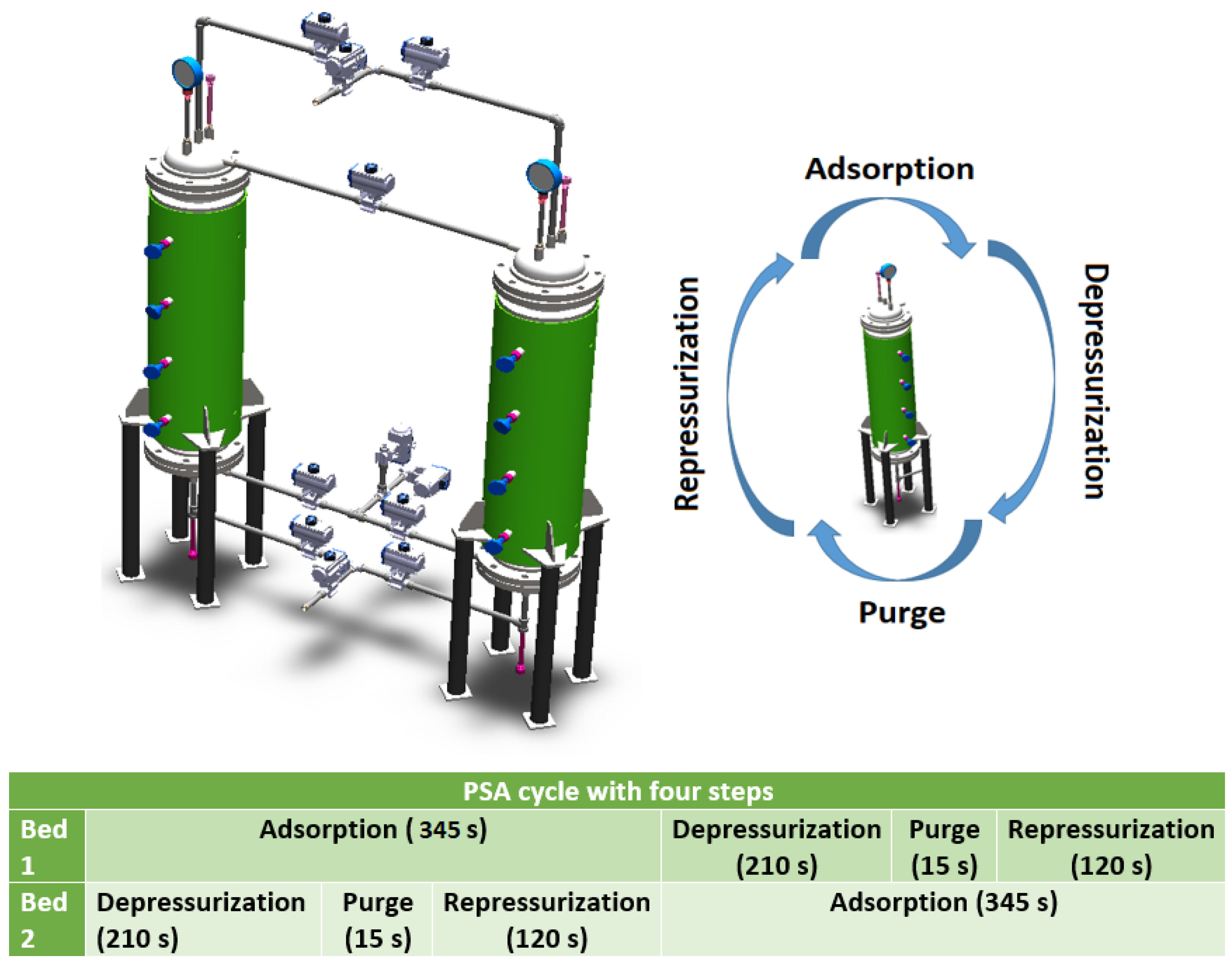
The PSA plant consists of two columns; its dimensioning and characteristics can be seen in Table 1 and Figure 1. The columns are connected through ten proportional valves; to achieve the operation of this process, it is necessary to define the nominal conditions of the startup. These data are shown in Table 2.

Table 1.
Characteristics and sizing of the packed bed.

Figure 1.
Steps and cycle time of the PSA plant.
Table 2.
Parameters of nominal starting conditions.
The PSA process is configured with four steps: adsorption, depressurization, purge, and repressurization. In this article, the PSA steps are simulated from a set of PDEs. These equations describe the matter, energy, momentum, and adsorption quantity equilibria within the adsorbent-packed bed. The following assumptions were considered in the PDEs:
- The gas phase behaves ideally.
- The gas phase instantaneously reaches thermal equilibrium with the adsorbent (solid).
- The Ergun equation can be used to describe the rolling moment.
- There is mass transfer between the gas and adsorbed phases.
- The rate at which the packed bed adsorbs is modeled using a Linear Driving Force approximation.
The adsorbent used for this innovative work is zeolite type 3A, and the Langmuir mathematical model (1) describes the adsorption isotherm.
where is the saturation charge for compounds i, are the Langmuir parameters, is the partial pressure and T is the temperature in the adsorption charge.
The isotherm parameters for the type 3A zeolite were obtained from [26]. Table 3 shows the isotherm parameters for zeolite.
Table 3.
Parameters of the Langmuir isotherm.
The mass balance for each component in the solid phase is given by Equation (2):
Flow over the solid surface is
The energy balance in the solid phase is given by Equation (4):
The Ergun equation is represented as follows (Equation (5)):
The mass transfer rate in the solid phase is described by the Linear Driving Force (LDF) model and is represented by Equation (6):
where
is the parameter in the Glueckauf expression.
The complete model considering the abovementioned assumptions is shown in Table A3, as well as its initial and boundary conditions for the sequence of steps established in Figure 1.
The PSA plant used in this work was taken from reference [26]. It is considered an experimental plant with operational conditions allowing greater bioethanol production.
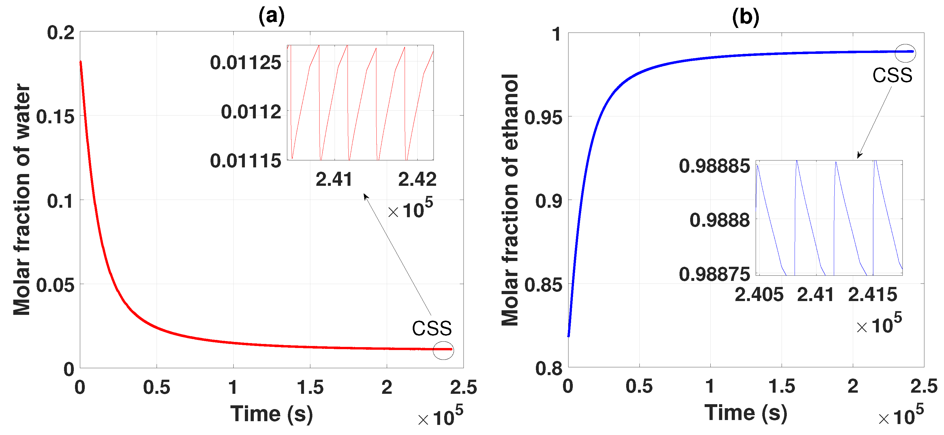
Figure 2 shows the behavior of the two compounds, which, based on the parameters established in Table 1, Table 2 and Table 3, separate and purify the ethanol and water mixture. After several cycles of operation, it is observed that the water begins to have a lower concentration and ethanol concentration increases; these data are collected as products of the two packed columns. After several cycles, the CSS is reached, generating an ethanol purity of 0.985 of molar fraction (99.5% wt). This obtained product meets the criteria and standards for use as biofuel.
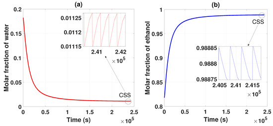
Figure 2.
(a) Separation and purification of water from startup to CSS. (b) Separation and purification of ethanol from startup to CSS.
3. Methodology
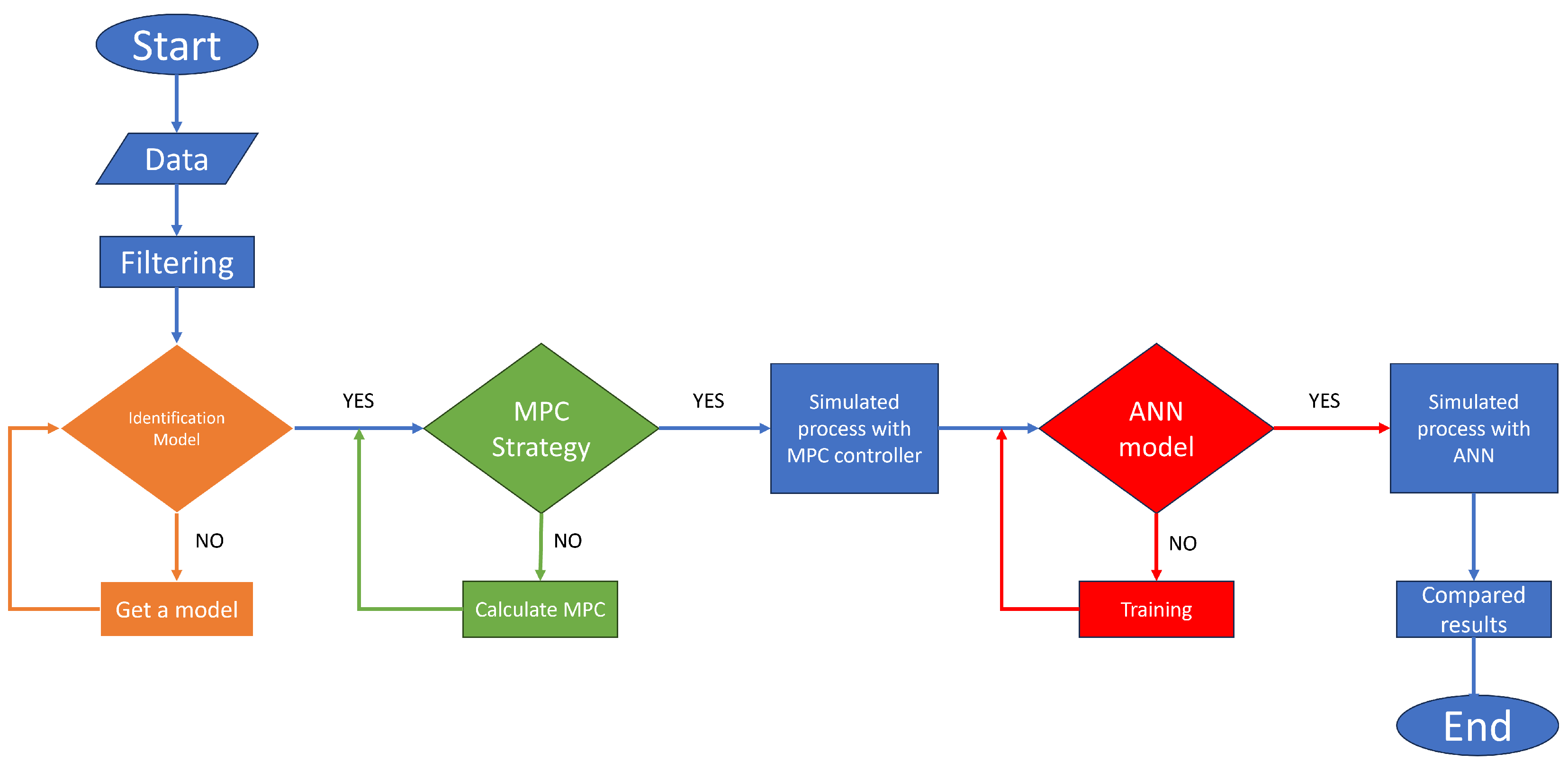
The proposed methodology to create an MPC based on an identified model using the input–output signals of the PSA plant is the following: obtaining the data, pre-treating the signals, obtaining a model using the system identification theory, designing an MPC controller with the identification model, simulating and collecting the signals to train the neural network, and controlling the PSA process using the ANN based on the MPC (see Figure 3).

Figure 3.
General methodology flowchart.
3.1. Data
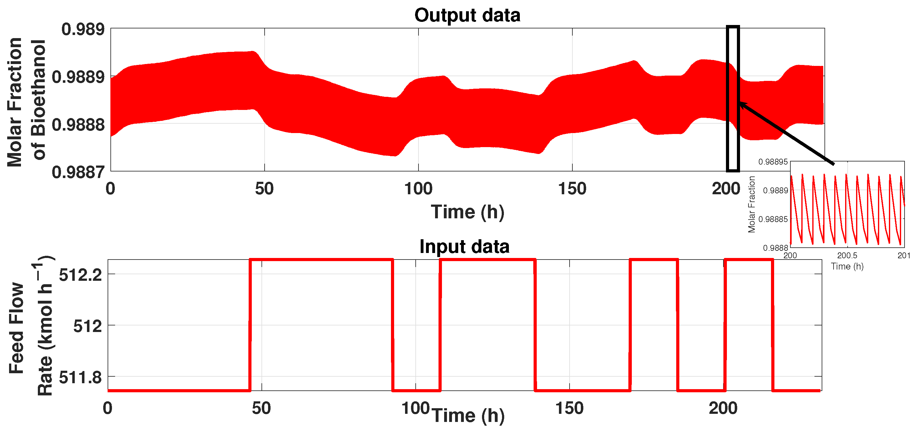
The PSA process has a cycle period and constant behavior, as described in the section before. Therefore, for modeling these patrons, we used the system identification technique described in [27]. First, we have the input–output data signals from the process. The input data represents the system’s flow rate, and the output signal represents the product’s purity, i.e., ethanol’s purity. Figure 4 shows the input and output signals. It can be observed that the purity has a cyclic period state, so designing a simple model that represents the behavior needs to be treated with a tool to maintain the behavior. The input data is a 5-bit PRBS signal (Figure 4), and the time duration pulse of 176,400 s (49 h) allows it reaching the stable state cyclic. The total duration of this signal is 833,176 s (232 h). The output data is the purity of ethanol of the PSA process obtained from the simulation of the input signal generated on Matlab ® and linked with the simulator of the plant in AspenOne ® for co-simulation.
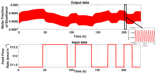
Figure 4.
Input–Output signals of the PSA process.
3.2. Pre-Treatment
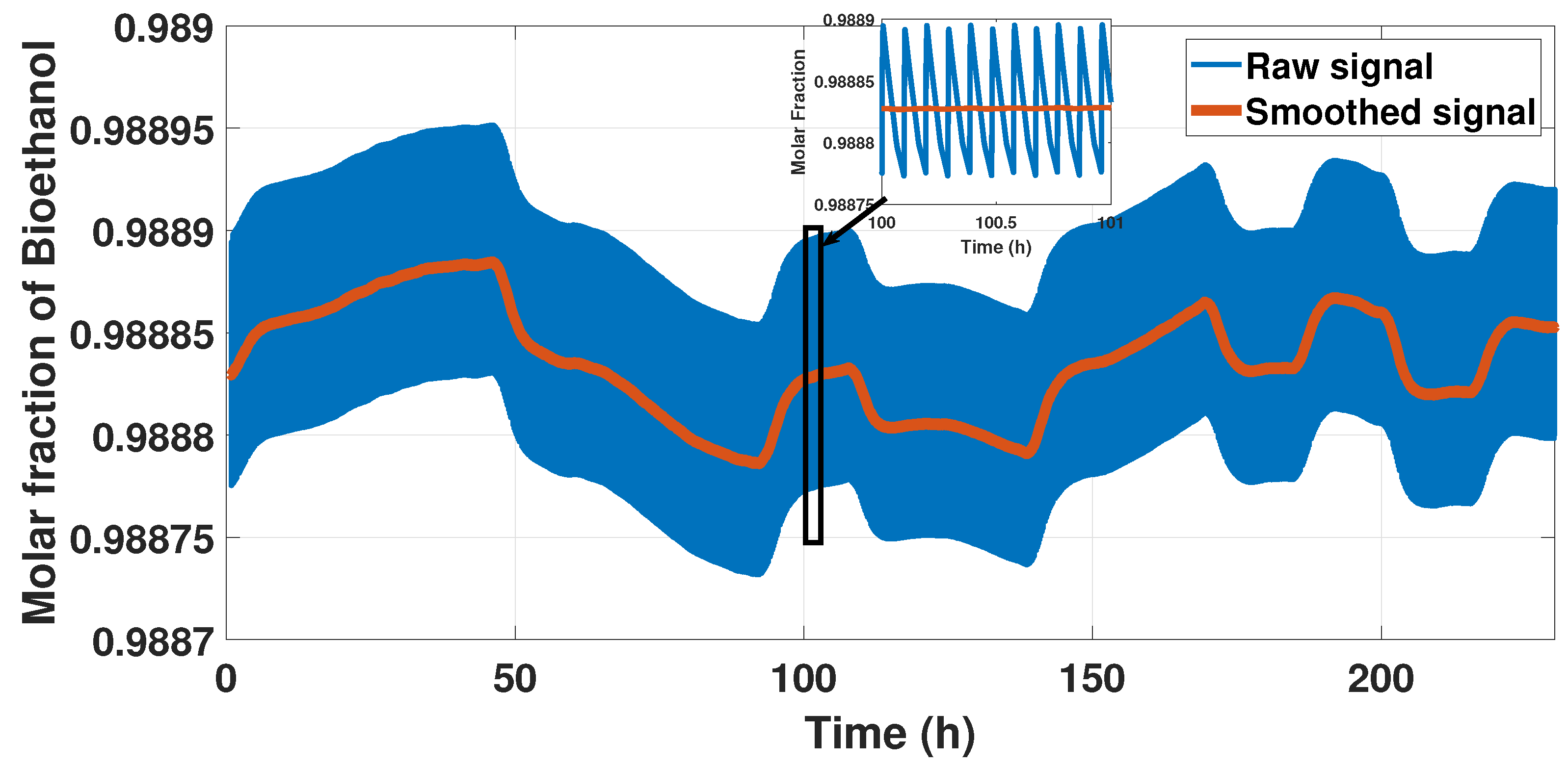
The model displayed a rigorous behavior because of the cycle form of the signal, so we smoothed the sign representing this behavior using a moving average method to reduce the cycle but not lose the behavior. We used the moving average with a windowing size of 100 s to reduce the computational cost and identified a model. Figure 5 shows the results of this pre-treatment.

Figure 5.
Output signal and smooth signal.
The identified model obtained with the input and output data of the PSA process is a Hammerstein–Wiener model, which was obtained with the MatLab toolbox. The input and output data used are shown in Figure 4.
To identify a reduced model, the Matlab ToolBox was used; the data entered into this tool were the feed flow (input) and the ethanol purity concentration (output). The output data were acquired from a PRBS that varies the flow with a ±5% described in [28]. When using the Matlab ToolBox, linear models were identified as a transfer function and state space; however, the approximation of the models obtained was less than 50% of the actual response of the PSA plant. For this reason, a non-linear model such as the Hammerstein–Wiener was used since this model from its input and output blocks (non-linear) allows a better approximation of 74% on the experimental data of the plant PSA. However, this work seeks to improve the approximation to have a prediction of the purity of bioethanol, and that is why Artificial Neural Networks are used.
3.3. Model
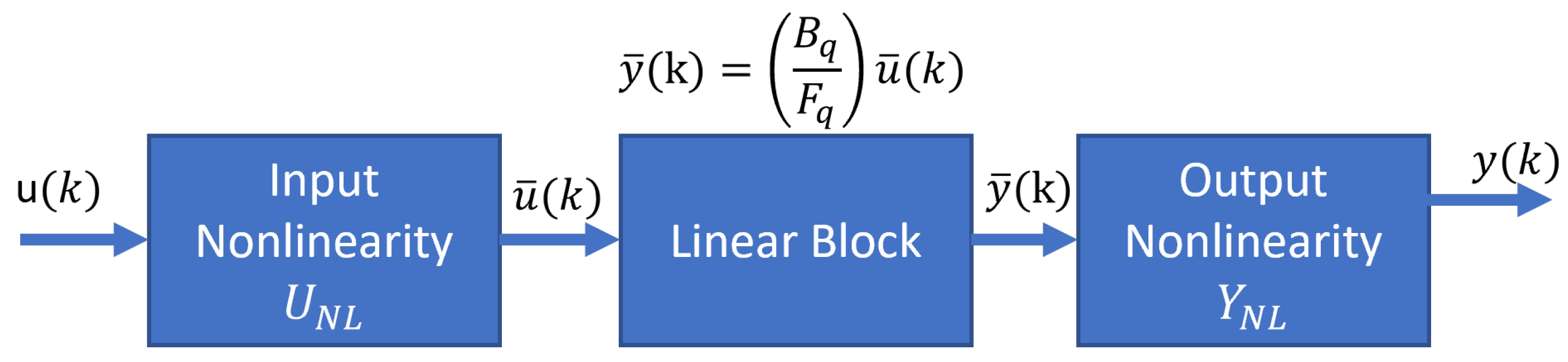
The responses of the PSA plant are nonlinear and display periodic temporal and spatial variations; because of that, we proposed a reduced model using the input and output signals. The system identification theory helps to find a model that relates the input variable (feed flow) and the output variable (ethanol purity) with a good approximation to the rigorous PSA model. In the literature, we found works related to the control of the PSA process using the Hammerstein–Wiener models [29]; however, the identification of the plant using this model poorly matches the plant performance, but we worked with a Hammerstein–Wiener model to predict the dynamics of the PSA for ethanol dehydration. The smoothed PSA process model has a Hammerstein–Wiener block structure composed of three blocks connected in series: a static nonlinear input block, a linear dynamic block, and a static nonlinear output block (Figure 6).
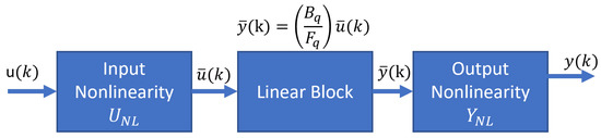
Figure 6.
Hammerstein–Wiener model.
The nonlinear input and output blocks were built with ten linear segments of a piece-wise defined Equations (8) and (10), respectively. The linear model is a transfer function with two zeros and three poles (Equation (9)). The linear model has an Output Error structure with a sampling time of 1 s. The final model is shown in Equations (8)–(10).
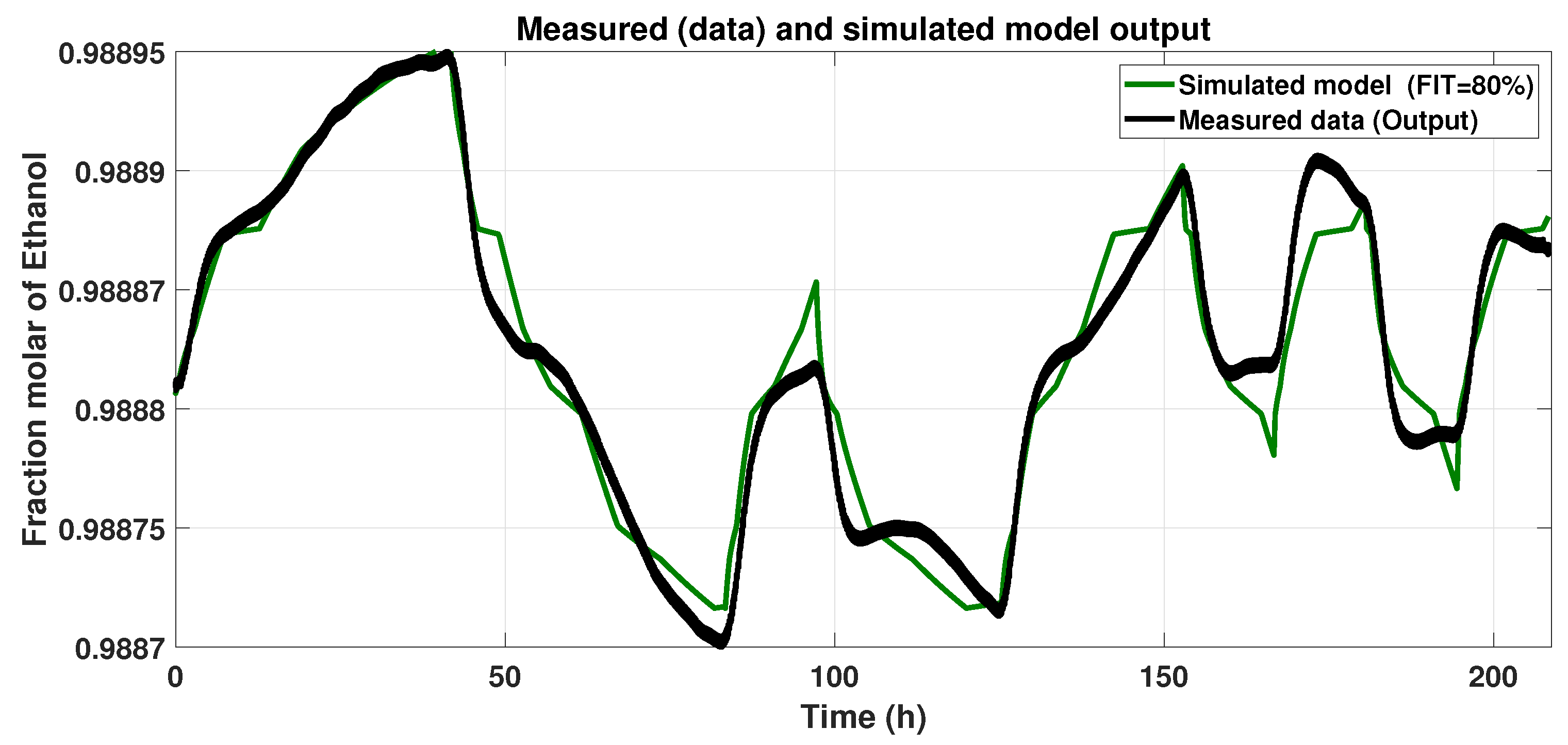
Figure 7 shows the Hammerstein–Wiener model response to the input signal (Figure 4) and the Smoothed Output Data. We assessed the Normalized Root Mean Square Error (NRMSE) (Equation (11)). After varying the numbers of piecewise linear equations in the input and output blocks, we looked for the maximum FIT, and the results with the model described below were 80%.
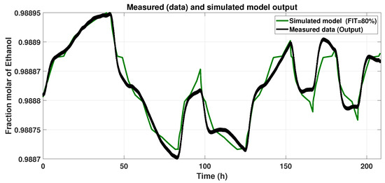
Figure 7.
Response of the Hammerstein–Wiener model to the input signal.
3.4. MPC
We designed an optimal MPC controller to track the reference and reject disturbances at the system input to maintain the purity product based on the dual-mode prediction and the close-loop paradigm [28]. The MPC controller is based on the linear model in the state space form without considering disturbances, in this case, of the form
where , k are the state, the control inputs, the system outputs, and the time instant. Model Equation (12) is obtained from the linear block of the Hammerstein–Wiener model; Equation (9) is converted to the space of states form, as follows:
A control law based on optimal feedback gain type LQ regulates the system and has the form
where and are the steady state values of the system. These values were obtained using Equation (15); in [30], a way to obtain and was explained, which is illustrated below.
where is the reference. The predictions for the control input based on the feedback gain K are
where is a compensation signal added to the control input. This signal is used to satisfy the restrictions of the predictive control. The value is a parameter that represents the controller’s degrees of freedom or the control horizon. is a decision variable that reduces the optimization’s computational load; also, large control horizons are not required with this variable. Thus, the model used for the prediction equations is
where and . This model represents the predictions of the states and control inputs. The prediction equations are given by:
The prediction vectors have the following dimensions: and , where is the prediction horizon.
When it comes to predictive control, one of the key factors to consider is the cost that needs to be optimized. This cost function is derived from the cost function of the infinite horizon. Using gain K, which is the feedback gain of optimal state LQ, we can determine that the cost function is a function of Lyapunov. This helps to ensure that the predictive control is stable, as guaranteed in [31]. The cost function itself is defined in terms of :
where , with . It is possible to suppress the term A in minimizing the cost function Equation (19), as it does not depend on the variable decision. This can help to simplify the optimization process and improve the efficiency of the predictive control system. Therefore, the cost function looks like this:
P is obtained from the solution of the following Lyapunov equation:
Another essential part of the MPC is definition of the restrictions. These can limit the control inputs, increments of the control inputs, the states, and the outputs. In general, the constraints have this form:
We substitute prediction Equations (18) into constraints Equation (22) resulting in the following restrictions:
where is a constant coefficient matrix that is calculated offline. Then, with cost function Equation (19) and constraints Equation (22), we obtain the following quadratic programming problem for optimal centralized predictive control:
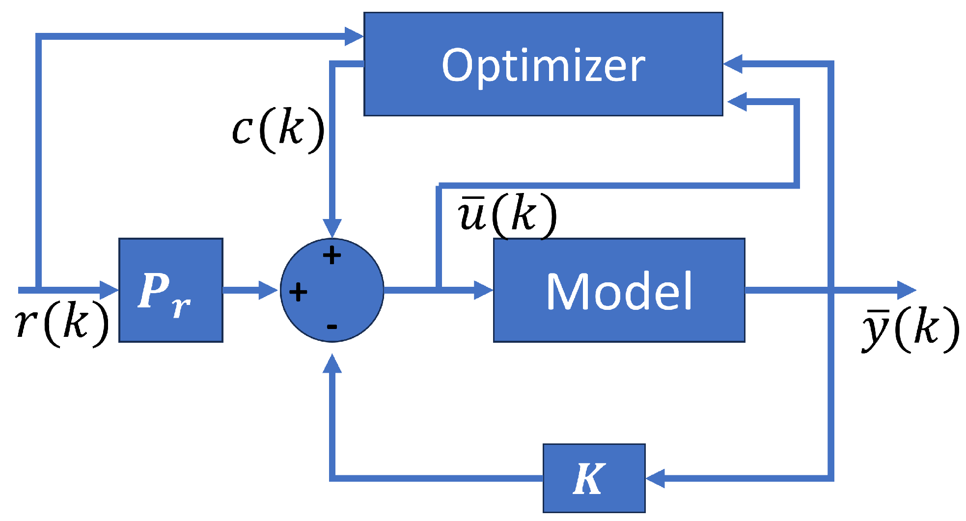
The optimizer of the Optimal MPC depends on the states, the control signal, and the reference. Also, the control signal is
Figure 8 shows the optimal MPC scheme with their components. The optimizer depends on the states, the control signal, and the reference.

Figure 8.
Optimal MPC structure.
As we mentioned before, the MPC uses the state of space of the linear block represented in Equation (13) with sampling time . To adjust the Optimal MPC controller, we use the linear block and the inverse function of the two static nonlinear blocks of the H-W model, as shown in Figure 9. The inverse functions are presented in Table A1 and Table A2.
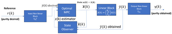
Figure 9.
MPC structure and the connection with the PSA process represented with the Hammerstein–Wiener system identification model.
The signal generated by the controller has constraints:
where is the signal generated by the Optimal MPC, restricted in the interval mentioned above. For generating the real input, i.e., values of the feed flow rate, we introduce the signal generated by the controller to the inverse non-linear block. Therefore, the real input is in the following interval:
Another consideration for the controller is in the output signal, which must be included in this interval:
In the considerations of output system , it is necessary to have restrictions in this way:
where is the output (molar fraction or purity obtained) of the PSA process. The constraint is that purity must not exceed 1.
To ensure optimal performance and achieve the desired purity in fewer cycle times before disturbances, it is important to tune the controller with the right parameters. These tuning parameters include the weight matrix of the states (R), the weight matrix of the control input (Q), the horizon of prediction of the control input (), and the horizon of prediction of the outputs (). There are several methods to tune the parameters of the MPC, like those shown in [32,33], but in our case, we use a heuristic method and observe that with the values of and , the state control signal and evolution are smooth (slow).
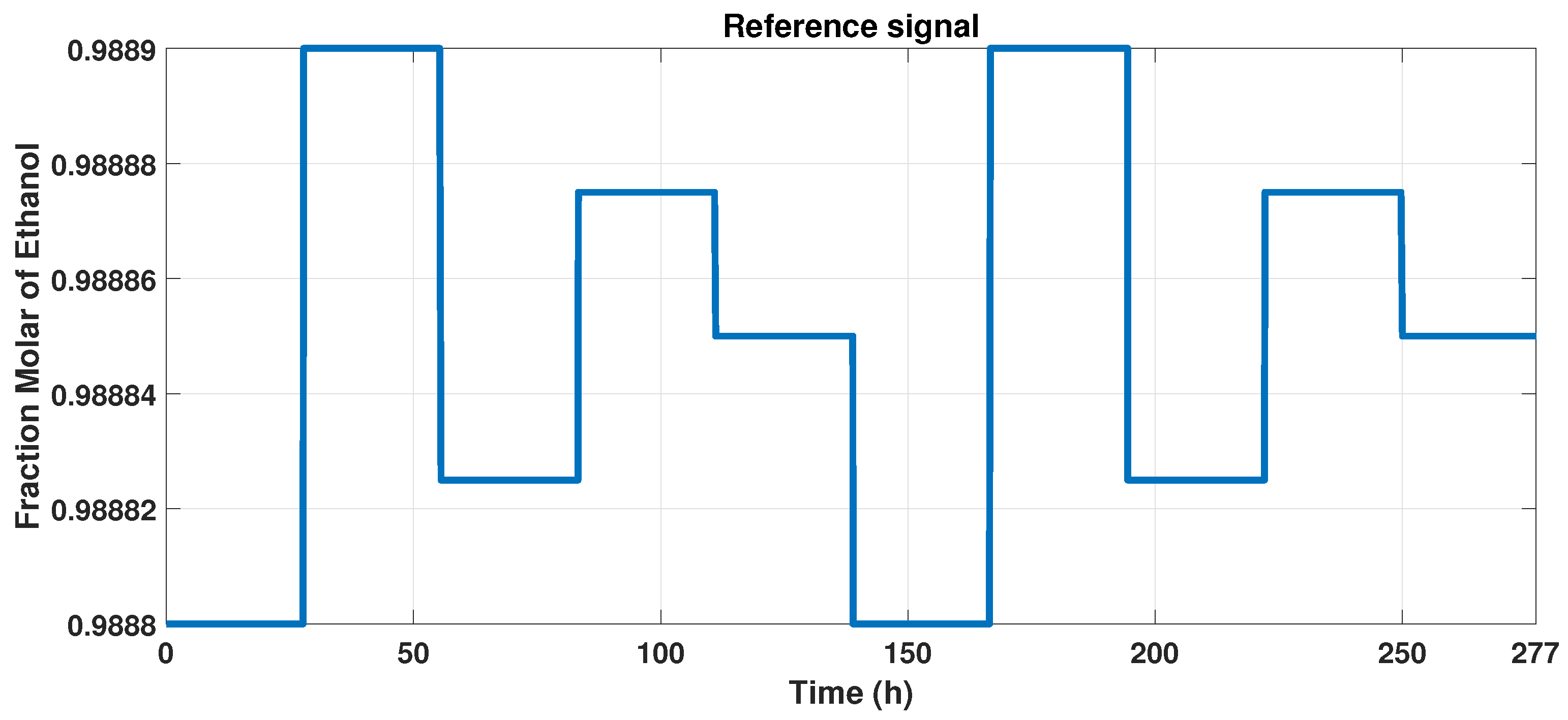
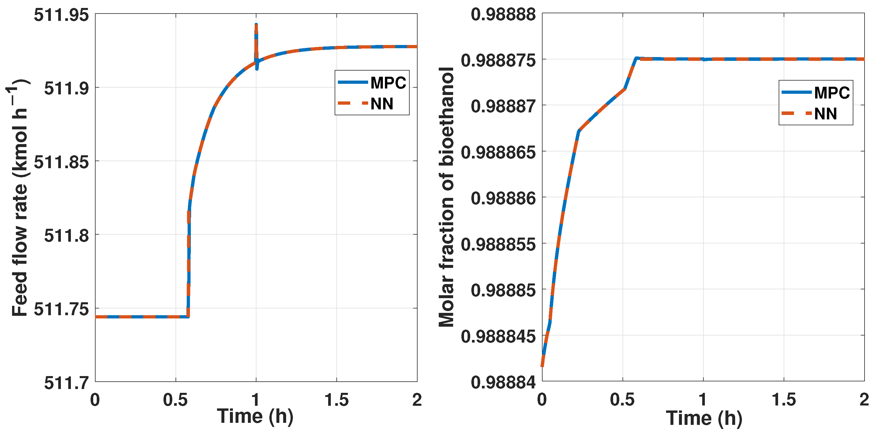
We track the reference output signal with the MPC controller so that we develop an input, varying the reference between the constraints of the observable variable, from 0.9888 to 0.9889 of molar fraction of bioethanol. Due to the purity, we maintain a narrow interval, which is observed in Figure 10.
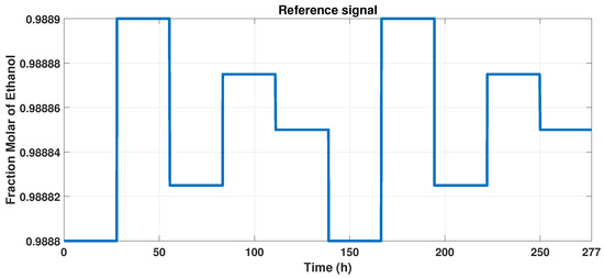
Figure 10.
Reference signal to MPC controller.
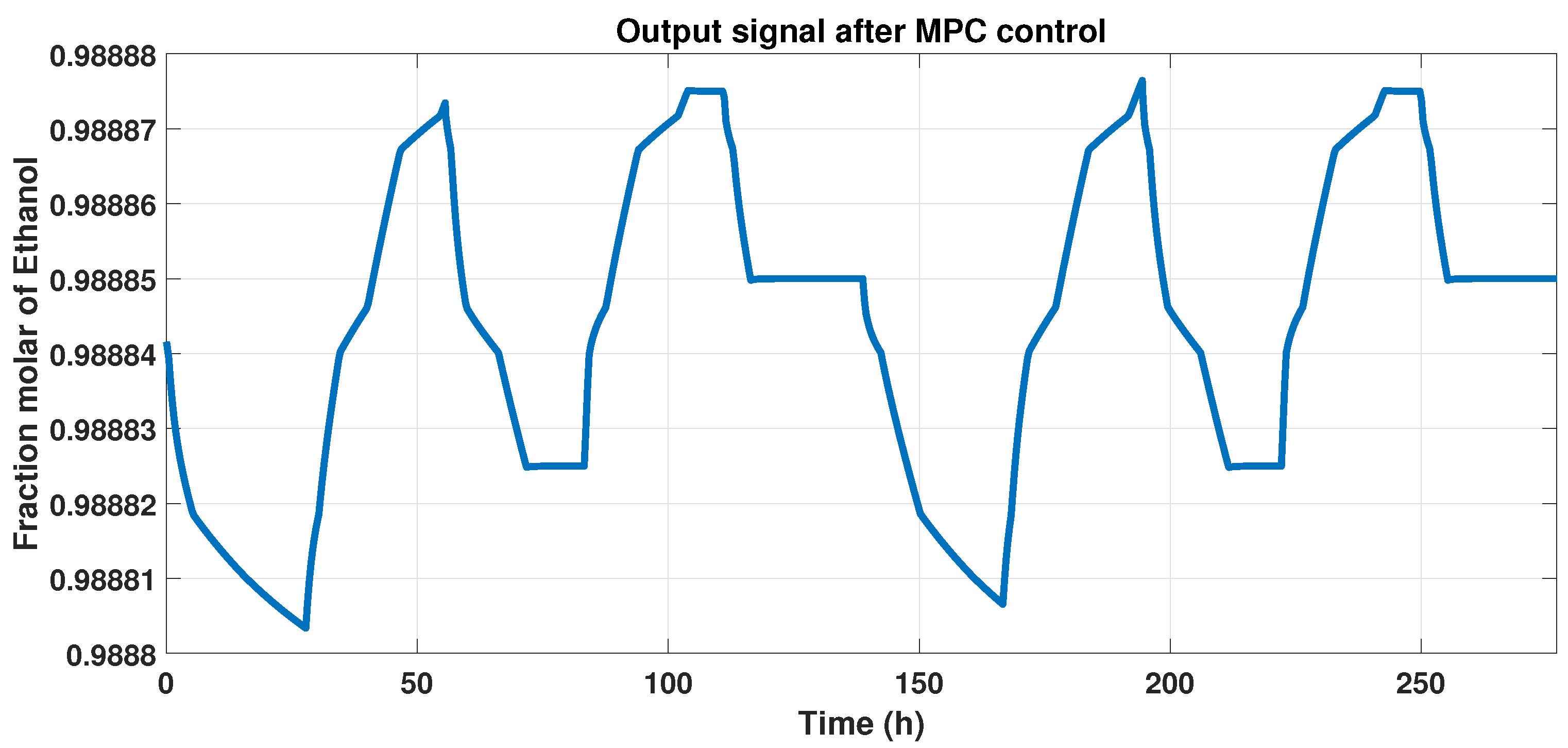
Figure 11 shows the behavior of the plant and the MPC controller, that is, the output signal, and represents the controlled purity of the systems that maintain 99% of ethanol with disturbances.

Figure 11.
Output signal that indicates the controlled purity with disturbances in the system.
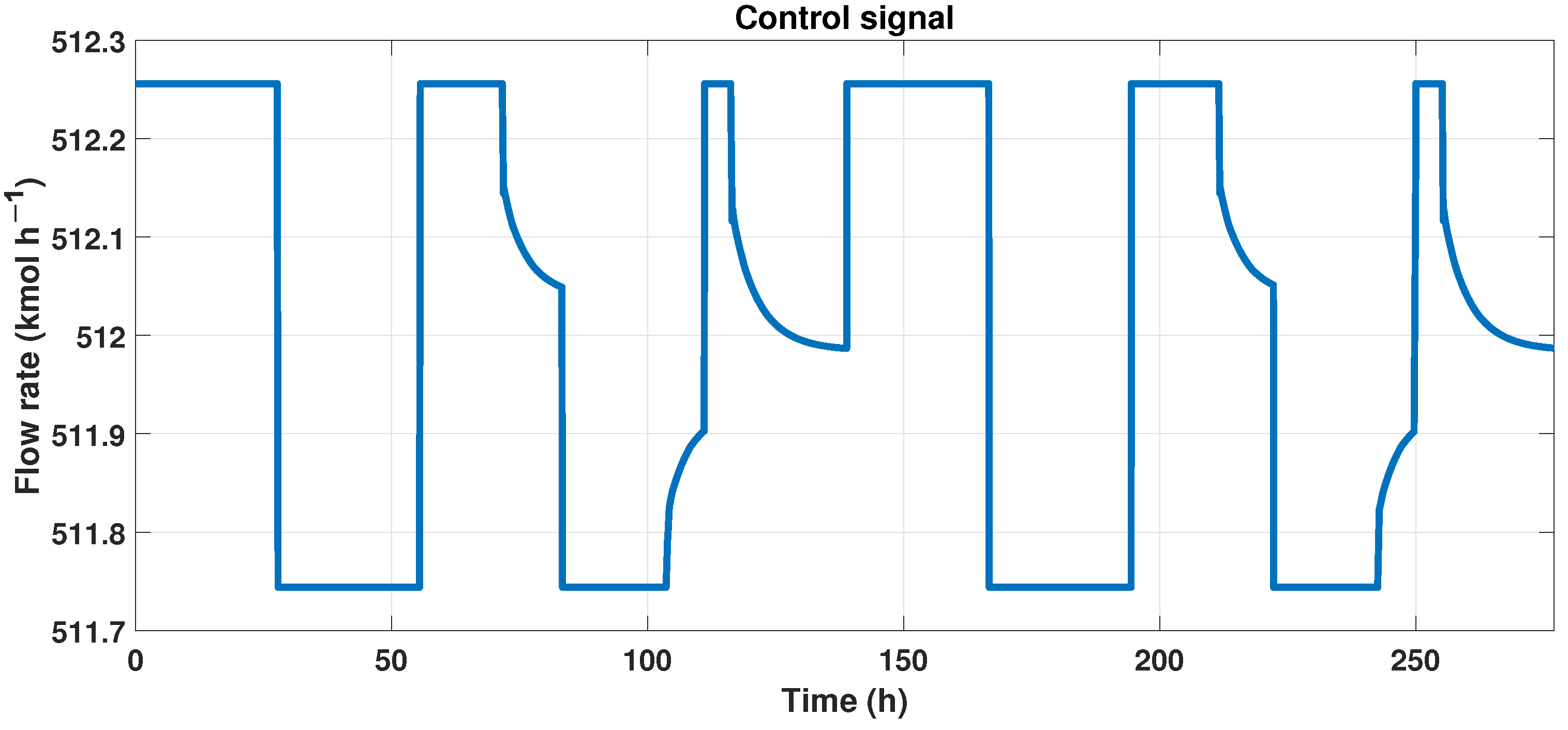
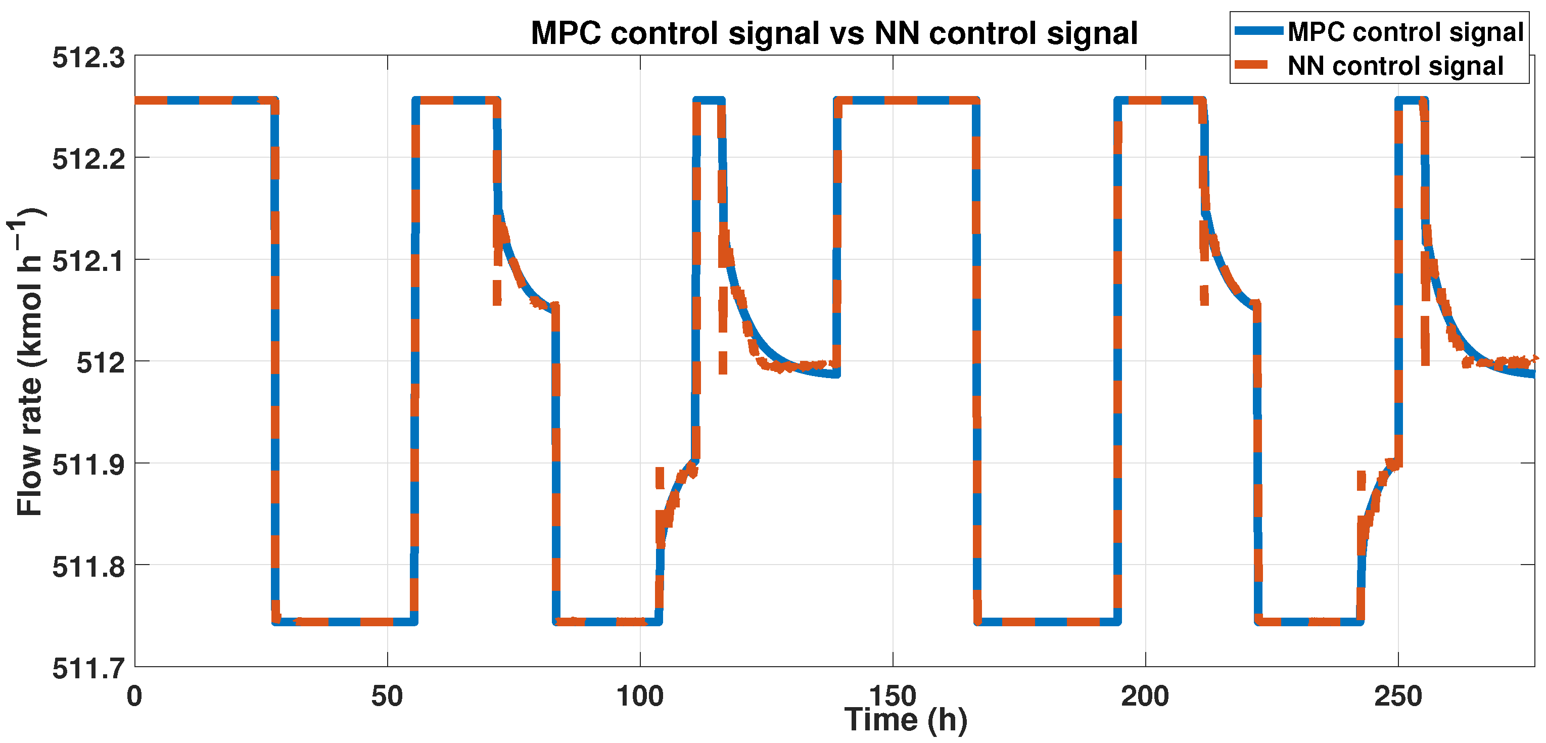
We need another signal to create a neural network that works as the MPC controller and is the control signal, and we observe this signal in Figure 12.
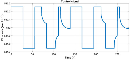
Figure 12.
Control signal (flow rate) of the MPC controller.
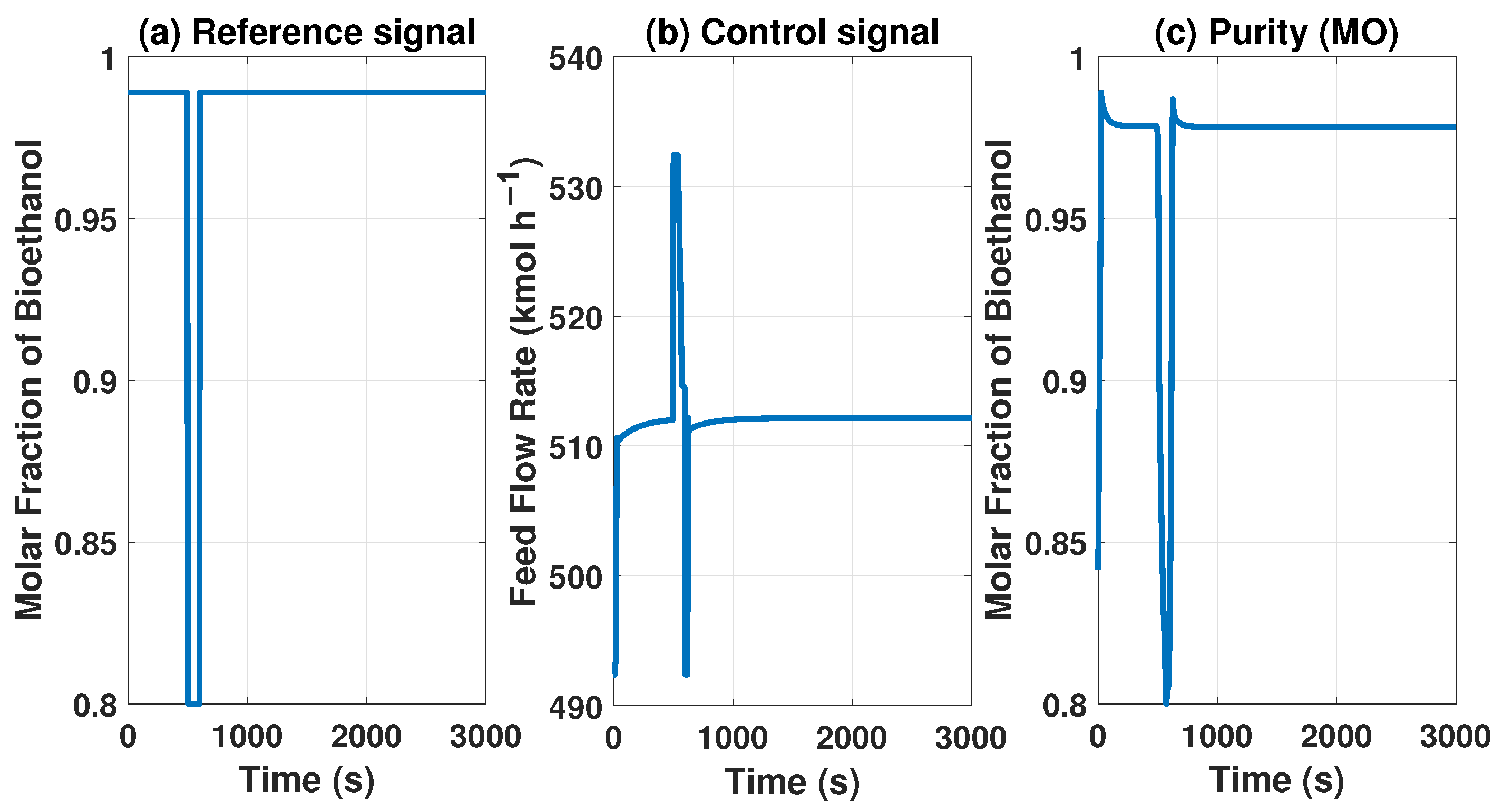
The MPC controller needs to maintain product purity despite disturbances at the inlet or outlet of the system. The model with the MPC controller can reach some uninteresting points because they do not comply with international biofuel standards. However, Figure 13 and Figure 14 show how it works if we need a lower concentration in purity, showing the behavior of our controller.

Figure 13.
Behavior of the control signal of MPC and purity of the product with a reference of 0.8 molar fraction of bioethanol.
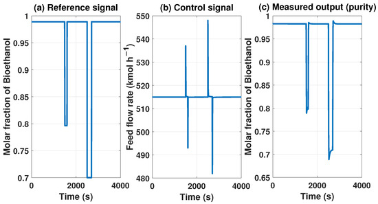
Figure 14.
Behavior of the control signal of MPC and purity of the product with a reference of 0.7 molar fraction of bioethanol.
3.5. Neural Network Based on MPC
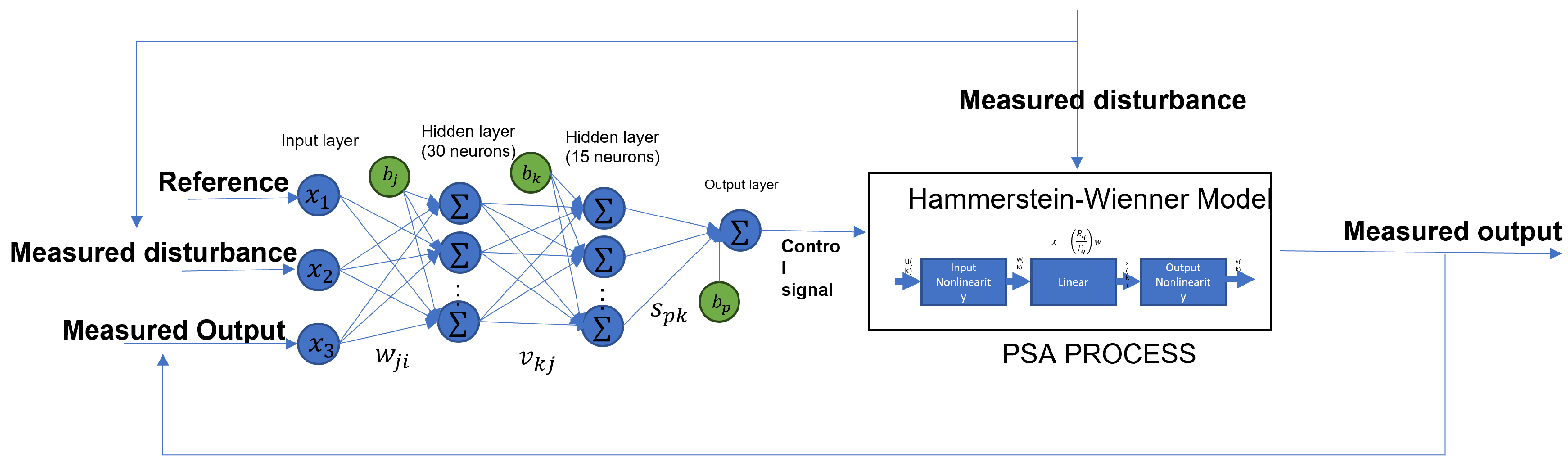
We need three input signals and one output signal to create the neural network based on the MPC controller. The necessary inputs are the reference, which the control needs to track; the disturbances, which, in this case of study, are noise in the input of the flow rate; and the output to feedback to the control. On the other hand, we need the control signal as the target of the ANN. Figure 15 shows the diagram of how the ANN based on the MPC works with the systems. The designed ANN model has an input layer, a hidden layer, and an output layer; the first layer has 30 neurons and uses the hyperbolic tangent sigmoid (tansig) activation function; the second layer has 15 neurons and a tansig activation function; the output layer has only one neuron with a linear transfer function. Also, each hidden layer has a bias. Algorithm 1 shows the steps to follow to get the ANN model.
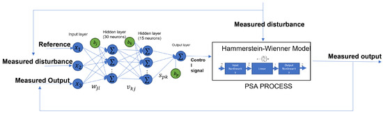
Figure 15.
Neural network based on the behavior of the MPC to control the PSA process.
The ANN represented in the Figure 15 can be expressed as
where is the output of the neural network, and are the weights in each layer, are the inputs of the ANN, are the bias in each layer, and is the activation function.
| Algorithm 1: Algorithm to build the neural network based on the MPC controller |
|
This ANN uses three input signals and one target signal, i.e., we need the reference, disturbance, and output values to approximate the control signal, so we use the signals shown in Figure 10 and Figure 12 that correspond to the reference and the output values. The disturbances are applied to the flow rate as white noise with . Figure 16 shows the trained ANN results that reach the fit of and a 0.0214 error using the RMSE formula.
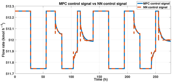
Figure 16.
Control signal of both controllers.
A neural network exhibits stability through its ability to maintain consistent and reliable predictions despite various inputs or perturbations. This stability is attributed to several factors in the network’s architecture and training process. Firstly, the use of activation functions with bounded outputs, such as the sigmoid or tanh functions, ensures that the network’s responses remain within a specific range, preventing wild oscillations or extreme values [34]. Utilizing large and diverse training datasets also contributes to stability by comprehensively representing the problem domain. Lastly, the iterative optimization process through stochastic gradient descent fine-tunes the network’s parameters, improving stability by gradually minimizing errors and converging toward an optimal solution [35]. These collective mechanisms fortify neural networks against variations and disturbances, enabling them to deliver consistent and dependable outputs.
We can mention that our neural network model is stable because of the following aspects:
- The dataset used for the training contains about 4,000,000 datapoints; is used for training, for validating, and for testing. Using large and diverse amounts of data contributes to the stability of the model.
- The Levenberg–Marquardt algorithm is efficient and strongly recommended. The main objective is to approximate the parameters to the optimal solution to resolve a quadratic function with small steps that take a long time to achieve convergence so that the gradient descent proves stability to the algorithm.
- The tansig activation function bounds the output. If we have a very deep neural network and bounded activation functions like this, the amount of error decreases dramatically after it is backpropagated through each hidden layer.
- Usign the small gain theorem [36],we guarantee uniformly ultimate boundedness stability, using the values of the weights of the NN; the result is 0.0082.
Also, we add disturbances in the input and output of the system to check the stability of the system. These tests are shown in the Results section.
4. Results and Discussion
This article’s primary purpose was to prove that a neural network can imitate the behavior of an MPC controller. For this objective, we obtained the targets of a ANN as the controller’s output, i.e., the controlled variable and its behavior after the MPC controller.
This work aimed to generate a neural network learned from an MPC controller behavior. How can the MPC control the purity of the product to control bioethanol purity in a PSA process that maintains the international standards to be used as biofuel? The MPC needs three signals:
- The feedback signal is the purity of the bioethanol.
- The disturbances are in the feed flow rate.
- The reference signal (purity desired).
We used several methods to verify the model’s performance index; in the first place, we applied the normalized root mean squared error (NRMSE) to the results of the ANN model and compared the data with those of the MPC model. The other index that we used was the root mean square error (RMSE).
These three signals are the inputs of the ANN. In this case, our ANN has three layers: an input layer with 30 neurons and a hyperbolic tangent sigmoid activation function in each one; a hidden layer with 15 neurons and the same activation function as the first layer; and an output layer with one neuron and a linear transfer function.
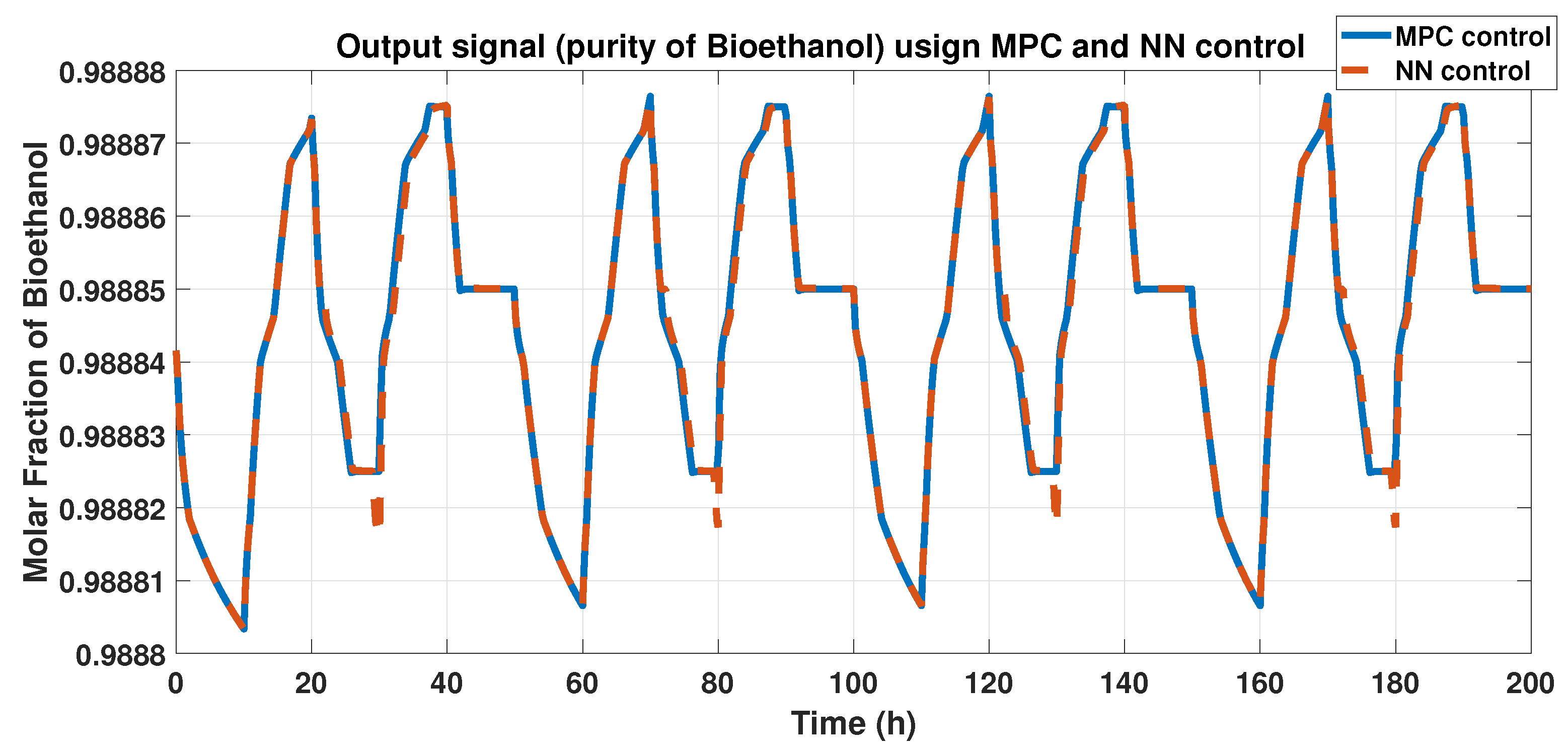
We compared the purity outputs using the MPC controller and the ANN model; we obtained a FIT using Equation (11) and 0.012 using the RMSE equation. Figure 17 shows these results.
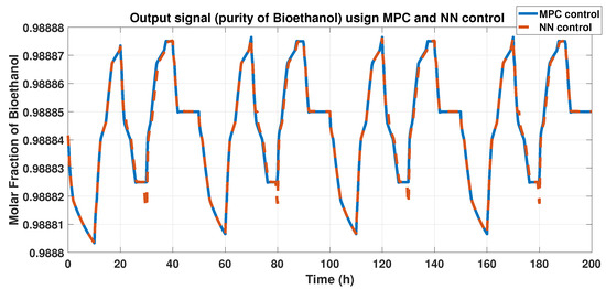
Figure 17.
Purity of bioethanol using the MPC and ANN controllers.
One big difference between the two controllers is that the ANN does not need many predictors, only one, compared with the MPC, which requires five predictors in both needed signals.
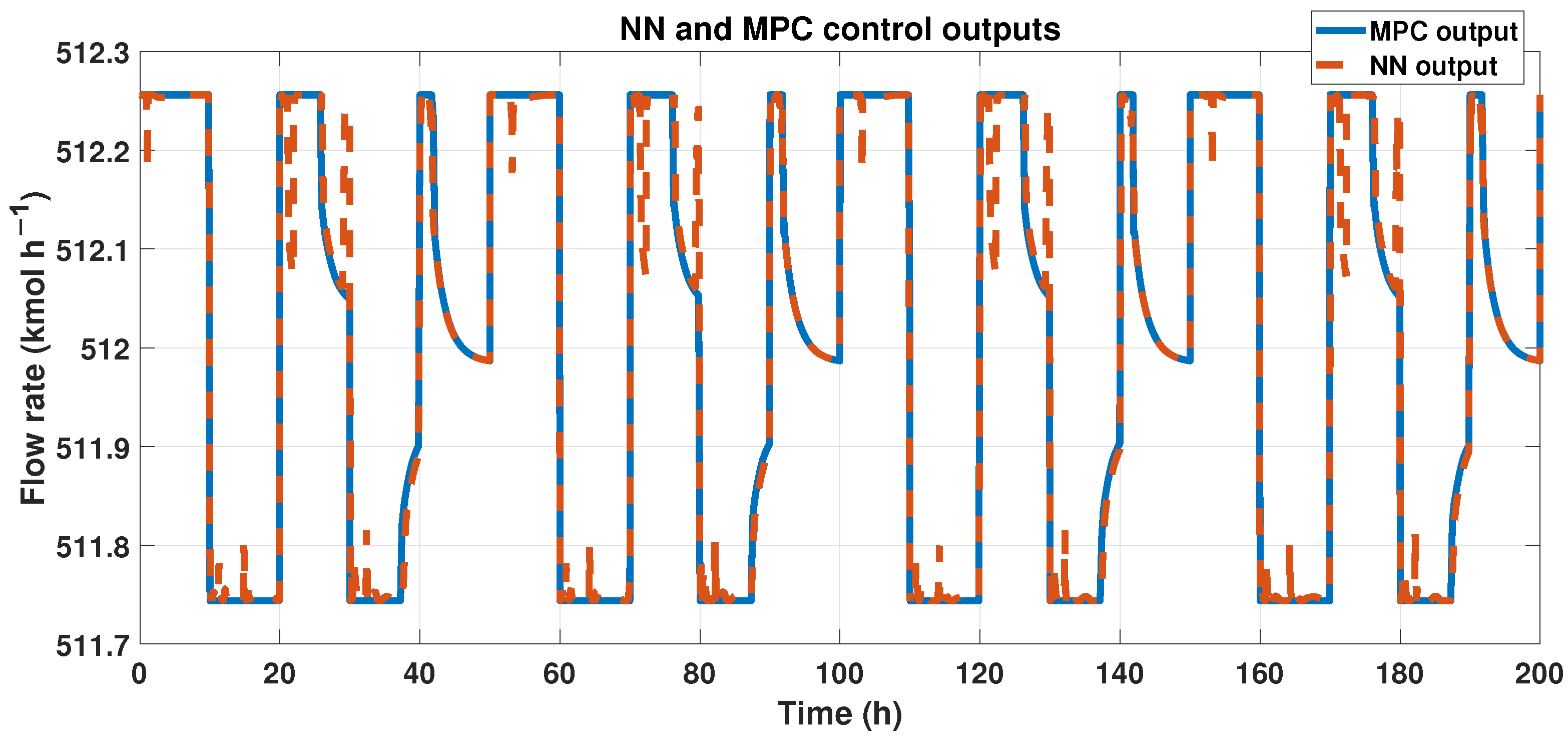
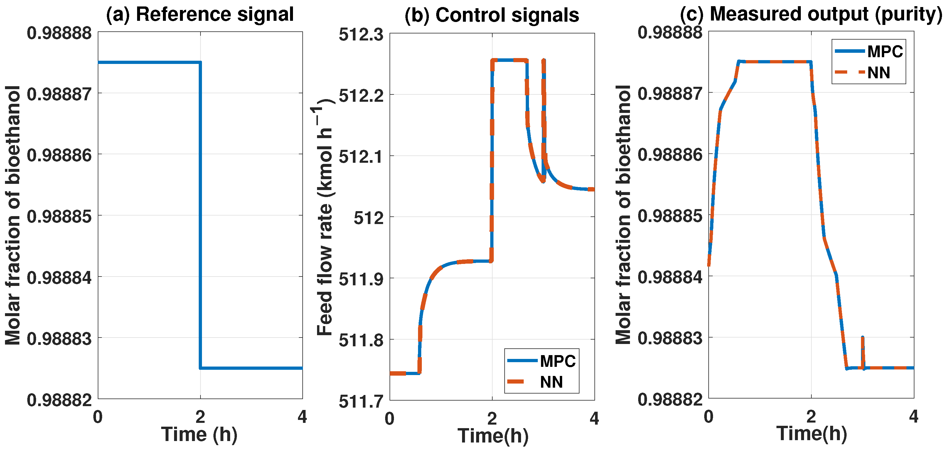
To achieve our goals, outputs from both the ANN and MPC must be similar. We can observe these results in Figure 18, showing the outcomes of ANN and MPC controllers. Also, we analyzed the fit using the corresponding equation. The signals had a 96% similarity, and using the RMSE, we obtained 0.1232 in error.
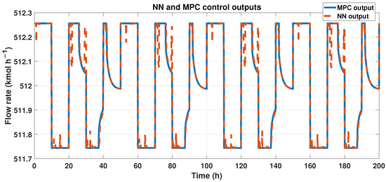
Figure 18.
Output signals from the MPC controller and the ANN-MPC controller.
ANN controller has stability. We probed the application of different disturbances in the plant system, and the measured disturbances applied were in the production temperature. This variable is strongly linked with the purity of the product; in [28], the authors presented a sensitivity analysis that reported that production temperature directly affects purity.
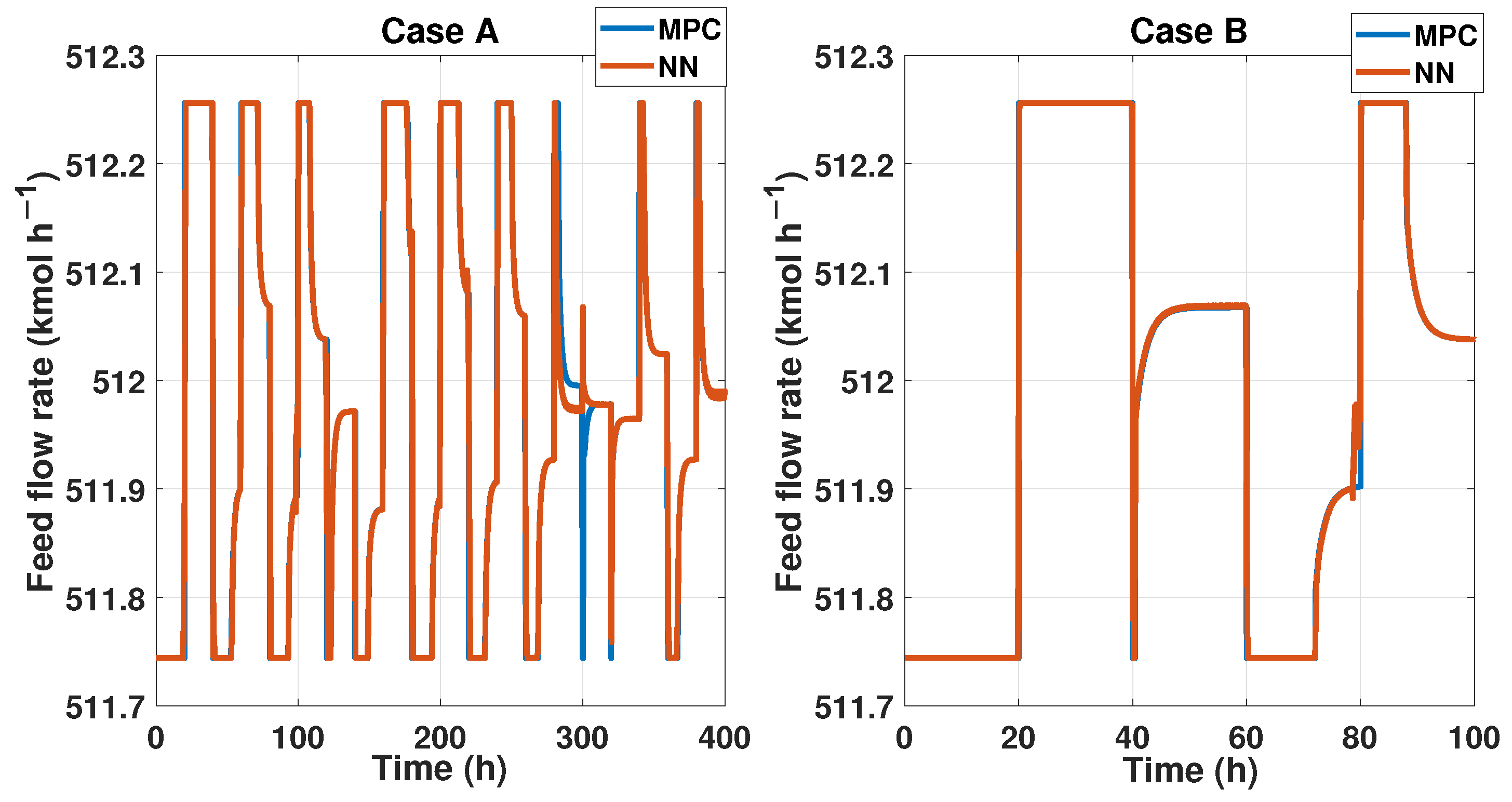
We probed the robustness of our ANN controller using different disturbances. We used a saw-tooth signal and a sine wave signal as a disturbance in the measured disturbance (noisy applied in production temperature). Figure 19 shows the reference signal which was generated using multiple steps; each step displayed about 30 min of difference. Also, we showed the noisy signal; this time, it was a sawtooth signal in the temperature with an amplitude of . Therefore, the purity results of the MPC and ANN controller were shown; using the NRMSE equation, we obtained a fit of , and using RMSE, the result was . Besides the ANN and MPC controller behavior shown in Figure 20 Case A, we obtained an RMSE of 0.0219 and a FIT = 96.72 %.
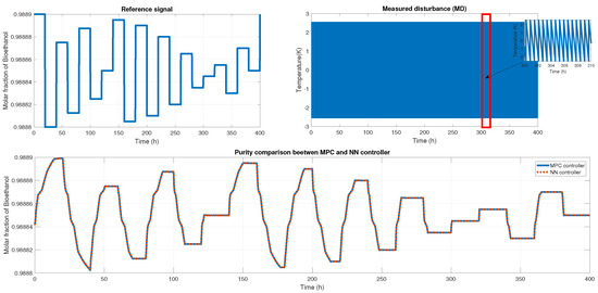
Figure 19.
(Top left) The reference signal; (Top right) the noisy signal that is a sawtooth signal; (Bottom) the comparison of purity from both controllers.
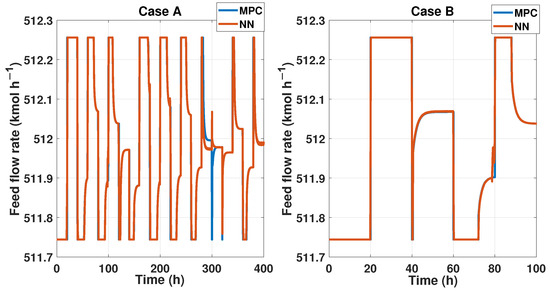
Figure 20.
(Left) The control signal of the controllers when a saw-tooth noisy signal is measured; (Right) the control signal from both controllers when a sine signal as noisy is observed.
Figure 21 shows another reference signal, another measured disturbance; in this case, the MD is a sine wave with an amplitude of 16 K, and both controllers maintain the purity and keep the reference tracking. The fit for this probe is and in RMSE. The MPC and ANN control signal is shown in Figure 20 Case B, where we obtained an RMSE of 0.0151 and FIT = 98.58%.
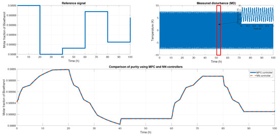
Figure 21.
(Top left) The reference signal; (Top right) The noisy signal that is a sine signal; (Bottom) the comparison of the purity from both controllers.
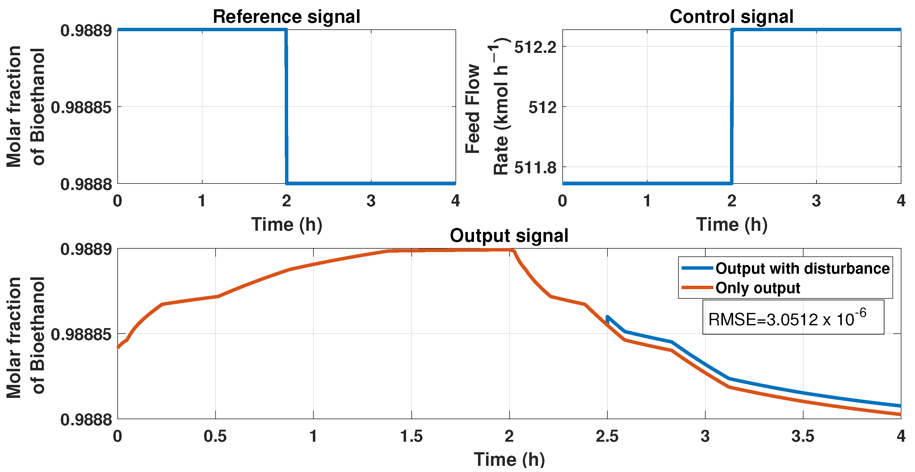
We included some tests to prove the stability of the ANN model by applying disturbances in the input and output of the systems. First, Figure 22 represents a disturbance of 10% in the output at the time 2.5 h. We observed an upset in the signal of the product because of the disturbance. Figure 23 represents the comparison between the output signal (purity of bioethanol) with an additive disturbance of −10% in the output of the process at the 3 h time and the signal without it. The upset observed in the purity caused by the output disturbance has the value of , determined using the RMSE equation.
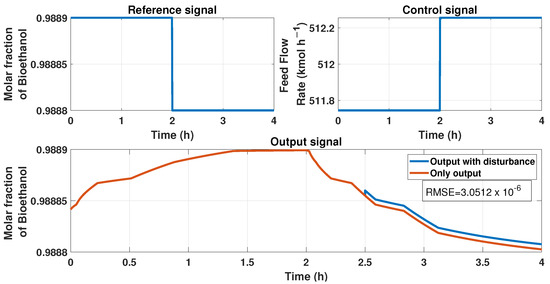
Figure 22.
This figure represents disturbance in the output signal, i.e., the purity signal at the time 2.5 h; the disturbance is about 10%. The top left figure displays the reference signal (purity desired), the top right figure shows the behavior of the ANN controller with and without output disturbance, and the bottom figure shows the purity behavior with and without disturbance.
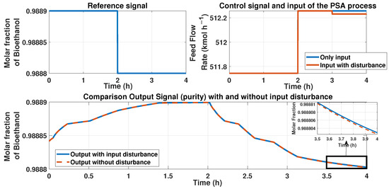
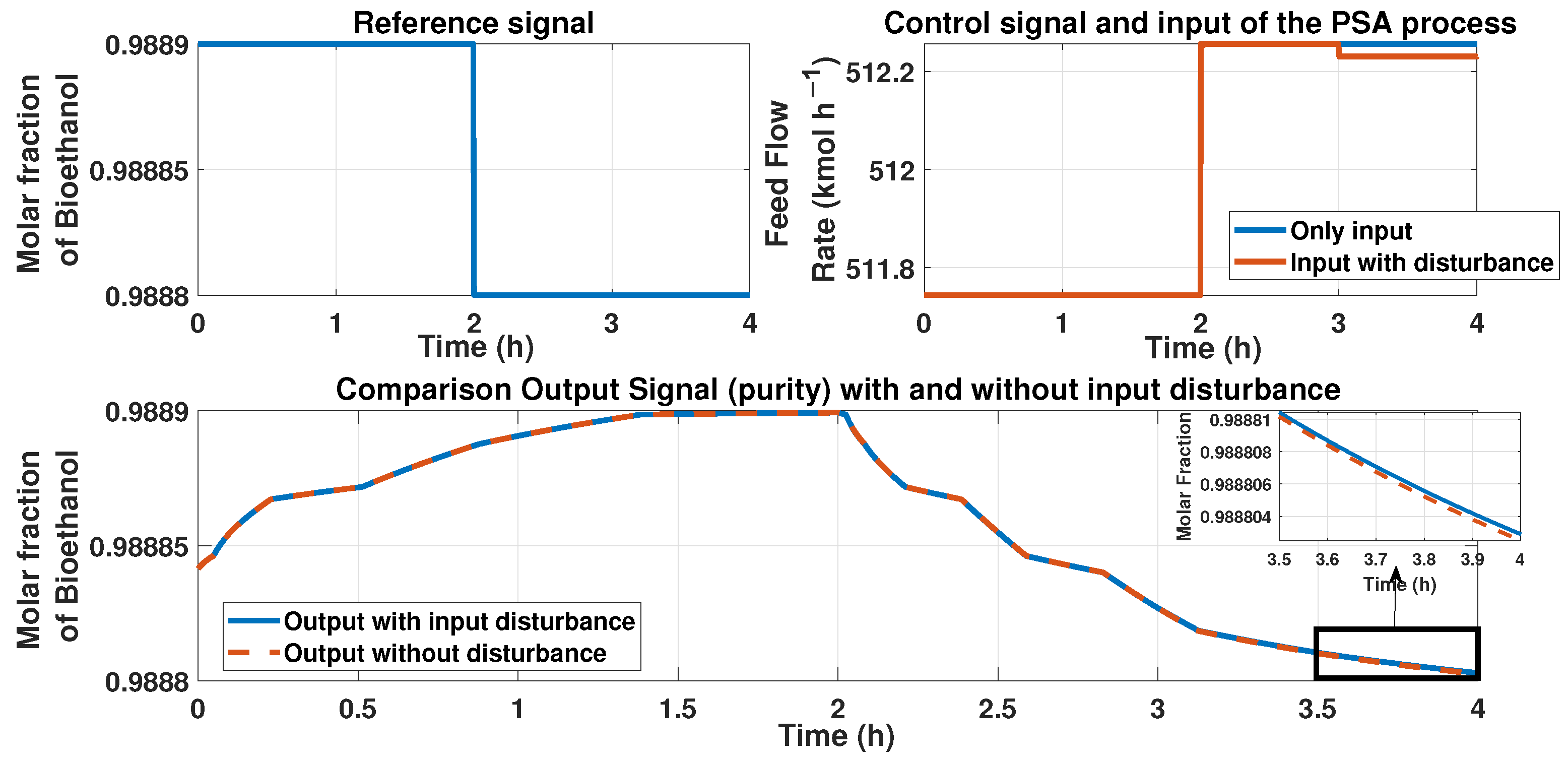
Figure 23.
This figure represents a disturbance in the input signal, i.e., the feed flow rate at the time 3 h; the disturbance is about −10%. The top left figure shows the reference signal (purity desired); the top right figure shows the behavior of the input of the PSA process and the control signal of the ANN controller and the additive disturbance of −10% in the input. The bottom figure shows the behavior of the purity with and without the disturbance. A zoom-in is presented in the 3 to 4 h time to show an error between signals.
The error caused by the disturbance in the feed flow rate has a value of . We used the RMSE equation to calculate this error.
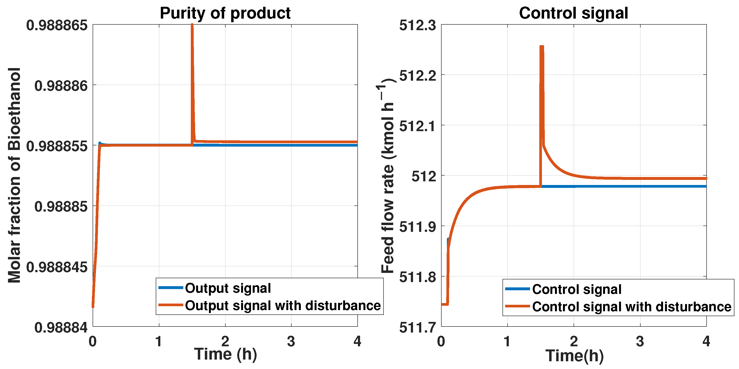
We put a reference signal constant with a 0.9889 molar fraction of bioethanol. Then, we implemented an additive disturbance in the purity product or an output signal of at a time of 1.5 h and observed the control’s behavior using the ANN. The comparison between the state with and without this disturbance is shown in Figure 24 on the left side. The response of the control signal from the ANN controller is shown in Figure 24 on the right side. We can observe that the control signal maintains a peak and then attempts to reach the stable value for tracking the reference after the disturbance at 1.5 h.
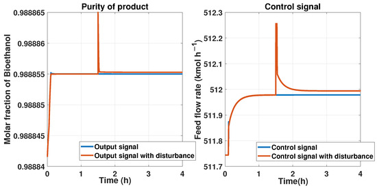
Figure 24.
Comparison between a disturbance in the output signal using the ANN controller and the PSA process and the signal without the disturbance. On the left is the purity of the product, and the disturbance is applied to this output. On the right is the behavior of the ANN controller.
The RMSE from the purity in the last test is about , and for the control signal it is 0.0214.
Comparison of the MPC and ANN Controllers
To compare both controllers, we applied them to the system disturbances in the input and output. Figure 25 compares the controllers with a disturbance in the output of 10%. We can observe similar behavior with the MPC and ANN controllers. The FIT reached by the ANN vs the MPc is about 99%.
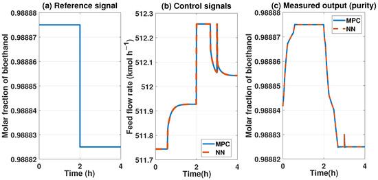
Figure 25.
Comparison between the two controllers, the MPC represented in blue lines and the ANN represented by red lines. The reference signal is the same for both controls, and disturbance is also the same.
We applied a disturbance in the input and control signals using a step of 10% of difference at 1 h time when we had a fixed reference setpoint of a 0.9885 molar fraction of bioethanol. Figure 26 shows this disturbance and the changes in the manipulated variable and the measured output.
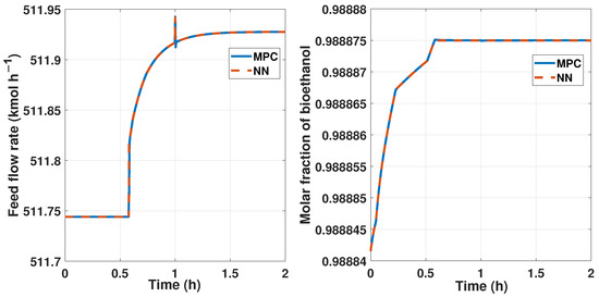
Figure 26.
Comparisonbetween the two controllers, the MPC represented in blue lines and the ANN controller represented by red lines. The reference signal is the same for both controllers. The left figure shows the input/control signal with a disturbance of 10%. The right figure shows the behavior of the purity signal of both controllers.
The ANN controller has some advantages concerning the MPC:
- The ANN does not need the inverse functions to control the system because of the training values.
- As we work in a restricted operating zone, the ANN controller saturates the control signal when the operating point leaves this zone and maintains stability, while with the non-linear MPC, this would not happen; it is entirely unstable.
- The ANN is very flexible because we can train it with new data; if the controller changes, we can train the ANN offline and work in the operating area.
The ANN robustness problem occurs when the process does not work at the operation points. In this case, the ANN controller saturates the control signal. On the other hand, the MPC controller becomes unstable when the optimization problem becomes infeasible due to the PSA process operating point at values near the 0.99 molar fraction of bioethanol needed to reach the international purity standards. Therefore, the ANN cannot present robustness problems because if the process deviates very far from the value of the international purity standard, it must stop completely.
5. Conclusions
In this research work, we showed an artificial neural network that represents the behavior of an MPC controller to maintain the purity of the product in the PSA process. We obtained a Hammerstein–Wiener model that describes the smoothed behavior of the process with a fit of . After that, we designed an MPC controller and then an ANN controller that learned the behavior using the three principal signals for an MPC controller: the reference signal (purity desired), the output signal, and disturbances (purity and feed flow rate variations). The ANN was trained using the Levenberg–Marquart algorithm and obtained a fit of in this step. To obtain the final results, we aborded identification system techniques to obtain the first model from the data of the PSA process.
It can be concluded that the neural network represents the MPC controller so that both controllers maintain the same purity at the 0.99 molar fraction of bioethanol. Also, both controllers attenuate the existing disturbances in the input and output. Furthermore, we can observe some variations in the control signal from the ANN controller. It occurs because the ANN has a similar behavior and not the exact behavior of the MPC controller.
Therefore, we can report substantial variations in the ANN control signal, but we maintain the product’s desired reference and molar fraction with disturbances in the input and output of the system.
We can guarantee the stability of our ANN controller with the following criteria: the activation function and the small gain theorem that allows boundedness, the data sets that are large enough, the algorithm that allows an optimal solution, and the tests with perturbations at the input and output signals of the PSA process.
In conclusion, the neural network control has the same performance and robustness. Both controllers manage to obtain a bioethanol purity of the 0.99 molar fraction, which is a purity that reaches international standards and can mitigate disturbances in that purity value.
For future work, the ANN controller will be implemented for other process control procedures, and new ANN structures to this process to realize more comparisons. Additionally, experimental results will be carried out with ANNs that update.
Author Contributions
Conceptualization, G.O.-T.; Methodology, F.D.J.S.-V.; Formal analysis, R.E.L.-P.; Investigation, M.R.-M.; Writing—original draft, M.R.-M.; Writing—review & editing, C.A.T.-C., H.A.-G., E.M.R.-V. and J.Y.R.-M.; Visualization, R.A.V.-M.; Supervision, J.Y.R.-M.; Funding acquisition, J.Y.R.-M. All authors have read and agreed to the published version of the manuscript.
Funding
This research received no external funding.
Acknowledgments
We want to thank the Centro Universitario de los Valles of the University of Guadalajara for the access and use of the laboratory of sustainable energy processes, in which the PSA pilot plant, the bioreactor, and boilers are located.
Conflicts of Interest
The authors declare no conflict of interest.
Nomenclature
| Particle surface, (m m) | |
| Molar concentration, (kmol m) | |
| Heat capacity of adsorbent, (MJ kmol K) | |
| Molecular diffusivity, (m s) | |
| Phase diffusivity adsorbed, (m s) | |
| Interparticle | |
| Intraparticle | |
| F | Flowrate, (kmol h) |
| Axial dispersion, (m s) | |
| Heat capacity, (MJ kg K) | |
| Heat transfer coefficient, (J s m K) | |
| i | Component index (water o ethanol) |
| Mass transfer rate, (kmol m(bed) s) | |
| K | Langmuir constant, (Pa) |
| M | Molar weight, (kg mol) |
| Isothermal parameters | |
| MTC | Mass transfer coefficient, (s) |
| Axial thermal conductivity, (W m K) | |
| OCFE2 | Orthogonal Collocation on Finite Elements |
| P | Pressure, () |
| Q | Isosteric heat, (J mol) |
| Adsorbed amount, (kmol kg) | |
| Adsorbed equilibrium amount, (kmol kg) | |
| R | Universal gas constant, (J mol K) |
| r | Adsorbent particle radius, (m) |
| t | Time, (s) |
| Gas temperature, (K) | |
| Solid temperature, (K) | |
| T | Temperature, (K) |
| Surface gas velocity, (m s) | |
| Molar fraction | |
| z | Coordinate of axial distance, (m) |
| Parameter in Glueckauf expression | |
| Particle shape factor | |
| Gas phase molar density |
Appendix A
Table A1.
Equations of the inverse function of the input nonlinear block.
Table A1.
Equations of the inverse function of the input nonlinear block.
| Inputs, () | Functions, | ||
|---|---|---|---|
| −0.0755169 | −0.065194044 | ||
| −0.065194 | −0.050708087 | ||
| −0.0507081 | −0.033337101 | ||
| −0.0333371 | −0.014359104 | ||
| −0.0143591 | 0.004947882 | ||
| 0.00494788 | 0.023305837 | ||
| 0.02330584 | 0.039436741 | ||
| 0.03943674 | 0.052062573 | ||
| 0.05206257 | 0.059905314 | ||
| 0.05990531 | 0.067748054 | ||
Table A2.
Equations of the inverse function of the output nonlinear block.
Table A2.
Equations of the inverse function of the output nonlinear block.
| Outputs, () | Functions, | ||
|---|---|---|---|
| −1.510686188 | −1.670584238 | ||
| −1.042026292 | −1.209422537 | ||
| −0.400755314 | −0.831366328 | ||
| 0.110743272 | −0.011239894 | ||
| 0.941357997 | 0.849759543 | ||
| 1.192160933 | 1.162594248 | ||
| 1.821986253 | 1.402923853 | ||
| 3.04779645 | 2.829778259 | ||
| 3.142302773 | 2.824853041 | ||
| 13.56097931 | 15.80409686 | ||
Table A3.
Equations used for the PSA plant: Use of initial and boundary conditions.
Table A3.
Equations used for the PSA plant: Use of initial and boundary conditions.
| Total mass balance | |
| Pressure drop | |
| Energy balance | |
| LDF approximation | |
| Adsorption isotherm | |
| Initial and boundary conditions: | |
| Step I (Adsorption): | Step III (Purge): |
| Step II (Depressurization): | Step IV (Represurization): |
References
- Renewable Fuels Association. 2023 Ethanol Industry Outlook. 2023. Available online: htts://ethanolrfa.org/library/rfa-publications (accessed on 1 August 2023).
- Wooley, R.; Ruth, M.; Sheehan, J.; Ibsen, K.; Majdeski, H.; Galvez, A. Lignocellulosic Biomass to Ethanol Process Design and Economics Utilizing Co-Current Dilute Acid Prehydrolysis and Enzymatic Hydrolysis Current and Futuristic Scenarios; Technical Report No. NREL/TP-580-26157; National Renewable Energy Lab (NREL): Golden, CO, USA, 1999. [Google Scholar] [CrossRef]
- Torres, O.; Morales, R.; Ramos Martinez, J.Y.; Valdez-Martínez, M.; Calixto-Rodriguez, J.S.; Sarmiento-Bustos, M.; Cantero, T.; Buenabad-Arias, C.A.; Active, H.M.; Torres, G.O.; et al. Active Fault-Tolerant Control Applied to a Pressure Swing Adsorption Process for the Production of Bio-Hydrogen. Mathematics 2023, 11, 1129. [Google Scholar] [CrossRef]
- Torres Cantero, C.A.; Pérez Zúñiga, R.; Martínez García, M.; Ramos Cabral, S.; Calixto-Rodriguez, M.; Valdez Martínez, J.S.; Mena Enriquez, M.G.; Pérez Estrada, A.J.; Ortiz Torres, G.; Sorcia Vázquez, F.d.J.; et al. Design and Control Applied to an Extractive Distillation Column with Salt for the Production of Bioethanol. Processes 2022, 10, 1792. [Google Scholar] [CrossRef]
- Singh, A.; da Cunha, S.; Rangaiah, G.P. Heat-pump assisted distillation versus double-effect distillation for bioethanol recovery followed by pressure swing adsorption for bioethanol dehydration. Sep. Purif. Technol. 2019, 210, 574–586. [Google Scholar] [CrossRef]
- Loy, Y.Y.; Lee, X.L.; Rangaiah, G.P. Bioethanol recovery and purification using extractive dividing-wall column and pressure swing adsorption: An economic comparison after heat integration and optimization. Sep. Purif. Technol. 2015, 149, 413–427. [Google Scholar] [CrossRef]
- Rumbo Morales, J.Y.; Ortiz-Torres, G.; García, R.O.D.; Cantero, C.A.T.; Rodriguez, M.C.; Sarmiento-Bustos, E.; Oceguera-Contreras, E.; Hernández, A.A.F.; Cerda, J.C.R.; Molina, Y.A.; et al. Review of the Pressure Swing Adsorption Process for the Production of Biofuels and Medical Oxygen: Separation and Purification Technology. Adsorpt. Sci. Technol. 2022, 2022, 3030519. [Google Scholar] [CrossRef]
- Martínez García, M.; Rumbo Morales, J.Y.; Torres, G.O.; Rodríguez Paredes, S.A.; Vázquez Reyes, S.; Sorcia Vázquez, F.d.J.; Pérez Vidal, A.F.; Valdez Martínez, J.S.; Pérez Zúñiga, R.; Renteria Vargas, E.M. Simulation and State Feedback Control of a Pressure Swing Adsorption Process to Produce Hydrogen. Mathematics 2022, 10, 1762. [Google Scholar] [CrossRef]
- Ullah, A.; Hashim, N.A.; Rabuni, M.F.; Mohd Junaidi, M.U. A Review on Methanol as a Clean Energy Carrier: Roles of Zeolite in Improving Production Efficiency. Energies 2023, 16, 1482. [Google Scholar] [CrossRef]
- Shang, J.F.; Ji, Z.L.; Qiu, M.; Ma, L.M. Multi-objective optimization of high-sulfur natural gas purification plant. Pet. Sci. 2019, 16, 1430–1441. [Google Scholar] [CrossRef]
- Basu, A.; Ali, S.S.; Hossain, S.K.; Asif, M. A Review of the Dynamic Mathematical Modeling of Heavy Metal Removal with the Biosorption Process. Processes 2022, 10, 1154. [Google Scholar] [CrossRef]
- Zong, T.; Li, J.; Lu, G. Identification of Hammerstein–Wiener Systems with State-Space Subsystems Based on the Improved PSO and GSA Algorithm. Circuits Syst. Signal Process. 2022, 42, 2755–2781. [Google Scholar] [CrossRef]
- Battisti, R.; Claumann, C.A.; Manenti, F.; Machado, R.A.F.; Marangoni, C. Machine learning modeling and genetic algorithm-based optimization of a novel pilot-scale thermosyphon-assisted falling film distillation unit. Sep. Purif. Technol. 2021, 259, 118122. [Google Scholar] [CrossRef]
- Karimi, S.; Ghobadian, B.; Najafi, G.; Nikian, A.; Mamat, R. Effect of operating parameters on ethanol-water vacuum separation in an ethanol dehydration apparatus and process modeling with ANN. Chem. Prod. Process. Model. 2014, 9, 179–191. [Google Scholar] [CrossRef]
- Renteria-Vargas, E.M.; Zuniga Aguilar, C.J.; Rumbo Morales, J.Y.; De-La-Torre, M.; Cervantes, J.A.; Lomeli Huerta, J.R.; Torres, G.O.; Vazquez, F.D.J.; Sanchez, R.O. Identification by Recurrent Neural Networks applied to a Pressure Swing Adsorption Process for Ethanol Purification. In Proceedings of the Signal Processing—Algorithms, Architectures, Arrangements, and Applications Conference Proceedings (SPA), Poznan, Poland, 21–22 September 2022; pp. 128–134. [Google Scholar] [CrossRef]
- Nogueira, I.B.; Ribeiro, A.M.; Requião, R.; Pontes, K.V.; Koivisto, H.; Rodrigues, A.E.; Loureiro, J.M. A quasi-virtual online analyser based on an artificial neural networks and offline measurements to predict purities of raffinate/extract in simulated moving bed processes. Appl. Soft Comput. 2018, 67, 29–47. [Google Scholar] [CrossRef]
- Smuga-Kogut, M.; Kogut, T.; Markiewicz, R.; Słowik, A. Use of Machine Learning Methods for Predicting Amount of Bioethanol Obtained from Lignocellulosic Biomass with the Use of Ionic Liquids for Pretreatment. Energies 2021, 14, 243. [Google Scholar] [CrossRef]
- Gopinath, A.; Retnam, B.G.; Muthukkumaran, A.; Aravamudan, K. Swift, versatile and a rigorous kinetic model based artificial neural network surrogate for single and multicomponent batch adsorption processes. J. Mol. Liq. 2020, 297, 111888. [Google Scholar] [CrossRef]
- Richard, K.F.; Azevedo, D.C.; Bastos-Neto, M. Investigation and Improvement of Machine Learning Models Applied to the Optimization of Gas Adsorption Processes. Ind. Eng. Chem. Res. 2023, 62, 7093–7102. [Google Scholar] [CrossRef]
- Leperi, K.T.; Yancy-Caballero, D.; Snurr, R.Q.; You, F. 110th Anniversary: Surrogate Models Based on Artificial Neural Networks to Simulate and Optimize Pressure Swing Adsorption Cycles for CO2 Capture. Ind. Eng. Chem. Res. 2019, 58, 18241–18252. [Google Scholar] [CrossRef]
- Ghaemi, A.; Karimi Dehnavi, M.; Khoshraftar, Z. Exploring artificial neural network approach and RSM modeling in the prediction of CO2 capture using carbon molecular sieves. Case Stud. Chem. Environ. Eng. 2023, 7, 100310. [Google Scholar] [CrossRef]
- Wu, X.; Cao, Z.; Lu, X.; Cai, W. Prediction of methane adsorption isotherms in metal–organic frameworks by neural network synergistic with classical density functional theory. Chem. Eng. J. 2023, 459, 141612. [Google Scholar] [CrossRef]
- Pai, K.N.; Nguyen, T.T.; Prasad, V.; Rajendran, A. Experimental validation of an adsorbent-agnostic artificial neural network (ANN) framework for the design and optimization of cyclic adsorption processes. Sep. Purif. Technol. 2022, 290, 120783. [Google Scholar] [CrossRef]
- Renteria-Vargas, E.M.; Zuniga Aguilar, C.J.; Rumbo Morales, J.Y.; Vazquez, F.D.J.S.; De-La-Torre, M.; Cervantes, J.A.; Bustos, E.S.; Calixto Rodriguez, M. Neural Network-Based Identification of a PSA Process for Production and Purification of Bioethanol. IEEE Access 2022, 10, 27771–27782. [Google Scholar] [CrossRef]
- Vo, N.D.; Kang, J.H.; Oh, D.H.; Jung, M.Y.; Chung, K.; Lee, C.H. Sensitivity analysis and artificial neural network-based optimization for low-carbon H2 production via a sorption-enhanced steam methane reforming (SESMR) process integrated with separation process. Int. J. Hydrog. Energy 2022, 47, 820–847. [Google Scholar] [CrossRef]
- Simo, M.; Brown, C.J.; Hlavacek, V. Simulation of pressure swing adsorption in fuel ethanol production process. Comput. Chem. Eng. 2008, 32, 1635–1649. [Google Scholar] [CrossRef]
- Ljung, L. System Identification: Theory for the User, 2nd ed.; Prentice-Hall PTR: Hoboken, NJ, USA, 1999. [Google Scholar]
- Rumbo Morales, J.Y.; López López, G.; Alvarado Martínez, V.M.; Sorcia Vázquez, F.d.J.; Brizuela Mendoza, J.A.; Martínez García, M. Parametric study and control of a pressure swing adsorption process to separate the water-ethanol mixture under disturbances. Sep. Purif. Technol. 2020, 236, 116214. [Google Scholar] [CrossRef]
- Rumbo Morales, J.Y.; Brizuela Mendoza, J.A.; Ortiz Torres, G.; Sorcia Vázquez, F.d.J.; Rojas, A.C.; Pérez Vidal, A.F. Fault-Tolerant Control implemented to Hammerstein–Wiener model: Application to Bio-ethanol dehydration. Fuel 2022, 308, 121836. [Google Scholar] [CrossRef]
- Muske, K.R.; Rawlings, J.B. Model predictive control with linear models. AIChE J. 1993, 39, 262–287. [Google Scholar] [CrossRef]
- Rossiter, J.A. Model-Based Predictive Control: A Practical Approach; CRC Press: Boca Raton, FL, USA, 2017. [Google Scholar] [CrossRef]
- Moumouh, H.; Langlois, N.; Haddad, M. A Novel Tuning approach for MPC parameters based on Artificial Neural Network. In Proceedings of the 2019 IEEE 15th International Conference on Control and Automation (ICCA), Edinburgh, UK, 16–19 July 2019; pp. 1638–1643. [Google Scholar] [CrossRef]
- Yamashita, A.S.; Martins, W.T.; Pinto, T.V.B.; Raffo, G.V.; Euzébio, T.A.M. Multiobjective Tuning Technique for MPC in Grinding Circuits. IEEE Access 2023, 11, 43041–43054. [Google Scholar] [CrossRef]
- Rasamoelina, A.D.; Adjailia, F.; Sinčák, P. A review of activation function for artificial neural network. In Proceedings of the 2020 IEEE 18th World Symposium on Applied Machine Intelligence and Informatics (SAMI), Herl’any, Slovakia, 23–25 January 2020; pp. 281–286. [Google Scholar] [CrossRef]
- Duchi, J.; Hazan, E.; Singer, Y. Adaptive Subgradient Methods for Online Learning and Stochastic Optimization. J. Mach. Learn. Res. 2011, 12, 2121–2159. [Google Scholar]
- Steil, J.J.; Ritter, H.J. Input-Output Stability of Recurrent Neural Networks with Delays Using Circle Criteria. In Proceedings of the International ICSC/IFAC Symposium on Neural Computation, Vienna, Austria, 23–15 September 1998; Heiss, M., Ed.; ICSC Academic Press: New York, NY, USA, 1998; pp. 519–525. [Google Scholar]


Disclaimer/Publisher’s Note: The statements, opinions and data contained in all publications are solely those of the individual author(s) and contributor(s) and not of MDPI and/or the editor(s). MDPI and/or the editor(s) disclaim responsibility for any injury to people or property resulting from any ideas, methods, instructions or products referred to in the content. |
© 2023 by the authors. Licensee MDPI, Basel, Switzerland. This article is an open access article distributed under the terms and conditions of the Creative Commons Attribution (CC BY) license (https://creativecommons.org/licenses/by/4.0/).