Numerical Investigation of Cavitating Jet Flow Field with Different Turbulence Models

Abstract

In numerous industries such as drilling, peening, cleaning, etc., a cavitating jet is adopted. However, it is challenging to simulate the cavitating flow field numerically with accuracy. The flow field of the organ pipe cavitation nozzle is simulated in this research using the RNG k−ε, DES, and LES turbulence models. The LES model can more accurately predict the periodic shedding of a cavitating cloud, which is basically consistent with the jet morphology captured with a high−speed camera. The flow pattern, cavitating cloud evolution and shedding period of a cavitating jet are analyzed. The findings demonstrate that the LES model produces a cavitating effect inside the nozzle that is superior to those produced by the RNG k−ε and DES models. The vortex rings in the diffusion section are simulated using the LES model, which accelerates cavitation. The cavitating clouds of the organ pipe nozzle show periodic evolutions, with stages of generation, development, shedding and collapse. The periodic shedding of the cavitating clouds exhibits a similar pattern in the vorticities simulated using the LES model, and the vorticities display the small-scale structures where the cavitating bubbles collapse. This study can provide a reference for the simulation of a cavitating jet and the analysis of the cavitating mechanism.

1. Introduction

The cavitation technique has been utilized for many varieties of applications [1]. An organ pipe cavitating nozzle is widely used in the fields of drilling [2,3], peening [4] and cleaning [5,6] because of its good cavitating performances. The internal flow of organ pipe cavitating nozzles is a high-speed complex flow accompanied by a vapor–liquid phase transition. It is difficult to obtain all the information of the cavitating flow field using experimental measurements [7]. Therefore, the numerical simulation method is needed to investigate its internal flow pattern. At present, most scholars carry out numerical simulations of cavitating nozzles using the RANS method. Han et al. [8] conducted a numerical simulation study on the organ pipe nozzle using the RANS method, and the results show that high-frequency pressure oscillations are generated when the jet flows through the organ pipe nozzle, which promotes the generation of cavitation. Wang et al. [9] studied the jet morphology and cavitation performances of self-excited oscillating nozzles adopting the RANS method, and they found that cavitation first occurred in the separation zone of the oscillation cavity, and the area of the cavitation was largest downstream of the nozzle outlet. The RANS approach was used by Yu [10], and Cai [11] et al. to optimize the output section’s shape of the organ pipe cavitating nozzle. They came to the conclusion that the acceptable length of the cylindrical section and the length and angle of the diffuser section may improve the cavitating jet’s performance. Dong et al. [12] numerically simulated the cavitating evolution of the angular nozzle and optimized the shape of the nozzle using the RNG k−ε model. Ran et al. [13] used the modified Reynolds-averaged k−ω model to simulate the cavitating morphologies in the hydrodynamic torque converter for different working conditions. However, due to the restraints of the used model, the RANS method can only simulate the time-averaged flow, and cannot accurately predict the spatial and temporal evolution of a cavitating cloud.

Large-eddy simulation (LES) can simulate the transient turbulent flow well. Researchers chose the LES approach to model the cavitating flow because it calculates large-scale and small-scale vortexes individually. As a result, the transient characteristics of the flow field and turbulent multi-scale flow characteristics may be correctly replicated. A more precise cavitation bubble shape was achieved by Yan et al. [14] implementing the LES to study the cavitation flow in a rotating sphere. Using the LES approach, Cheng et al. [15] quantitatively studied the cavitation flow in the tip leakage vortex (TLV) surrounding a hydrofoil. The numerical results are consistent with the findings of the experiments. The radius of the TLV is significantly impacted by cavitation. Xue et al. [16] adopted the LES model based on the dynamic sub-grid-scale stress model (DSM) to study the cavitation inside a diesel nozzle, and obtained the influence of the nozzle inlet filleting and fluid transition on cavitating inception. Using the RANS, RANS-LES, and LES methods, respectively, under elevated pressures, Yang [17,18] simulated the flow field of a submerged cavitating water jet. A few of the simulation findings and experimental results were compared. It was observed that the simulation results used under the RANS model differed from the actual flow field, and the numerical simulation results achieved via the RANS-LES and LES models agreed with the test results. The cavitating flow of the organ pipe nozzle was simulated by Wang et al. [19] adopting the unsteady DES model. Akira et al. [20] studied the vortex flow generated by the diesel nozzle with the LES method, and found that the LES could simulate the vortex structures better by comparing the results of this with the measured results. Trummler [21] studied the factors influencing the periodic shedding of the stepped nozzle’s cavitating clouds using the implicit LES method, and found that the condensation shock triggered the shedding of cavitating clouds. Ge [22] examined the variables influencing cavitation length and shedding frequency as well as the impact of temperature on cavitating performance.

The RANS method is computationally efficient, and the LES method can better simulate the cavitating flow pattern. However, there are fewer systematic analyses of the flow field and cavitating characteristics using different turbulence models for the organ pipe cavitating nozzle at lower pressures. As a consequence, this research integrates the RNG k−ε, DES, and LES with WALE models to simulate the cavitating jet of the organ pipe nozzle with a lower pressure and assesses the applicability of the various turbulence models for simulating a flow field and the process of a cavitating jet.

2. Numerical Methods

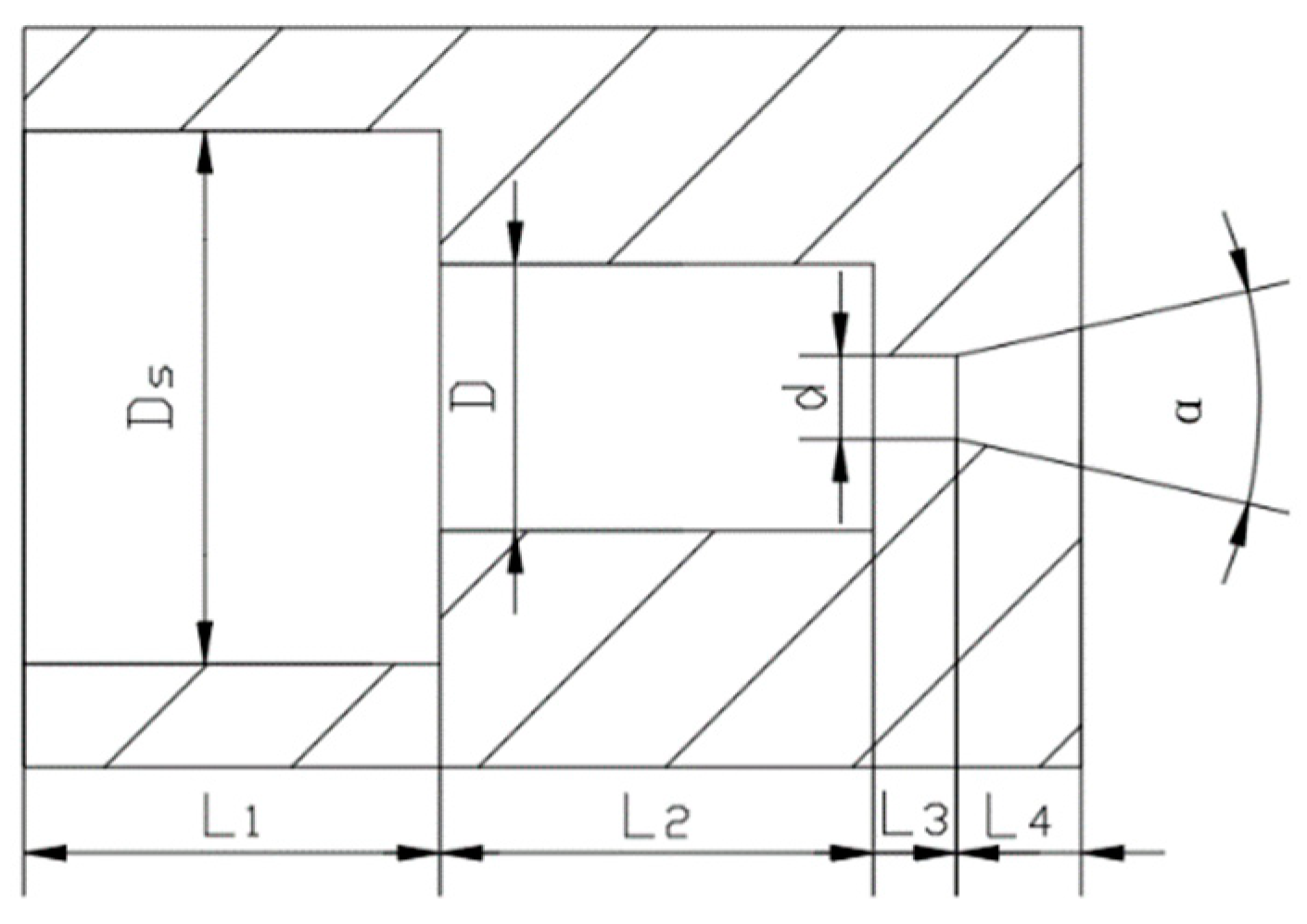
2.1. Geometry of Organ Pipe Nozzle

The geometry of the organ pipe cavitating nozzle is depicted in Figure 1 and is in accordance with that in earlier research [10,23]. The precise geometric specifications are presented in

Table 1. The structure characteristics of the organ pipe nozzle.

Ds (mm)	D (mm)	d (mm)	L1 (mm)	L2 (mm)	L3 (mm)	L4 (mm)	α (°)
6.4	3.2	1	5	5.2	1	1.5	12.5

, and the nozzle diameter, d, is 1 mm.

2.2. Grid and Independence Validation

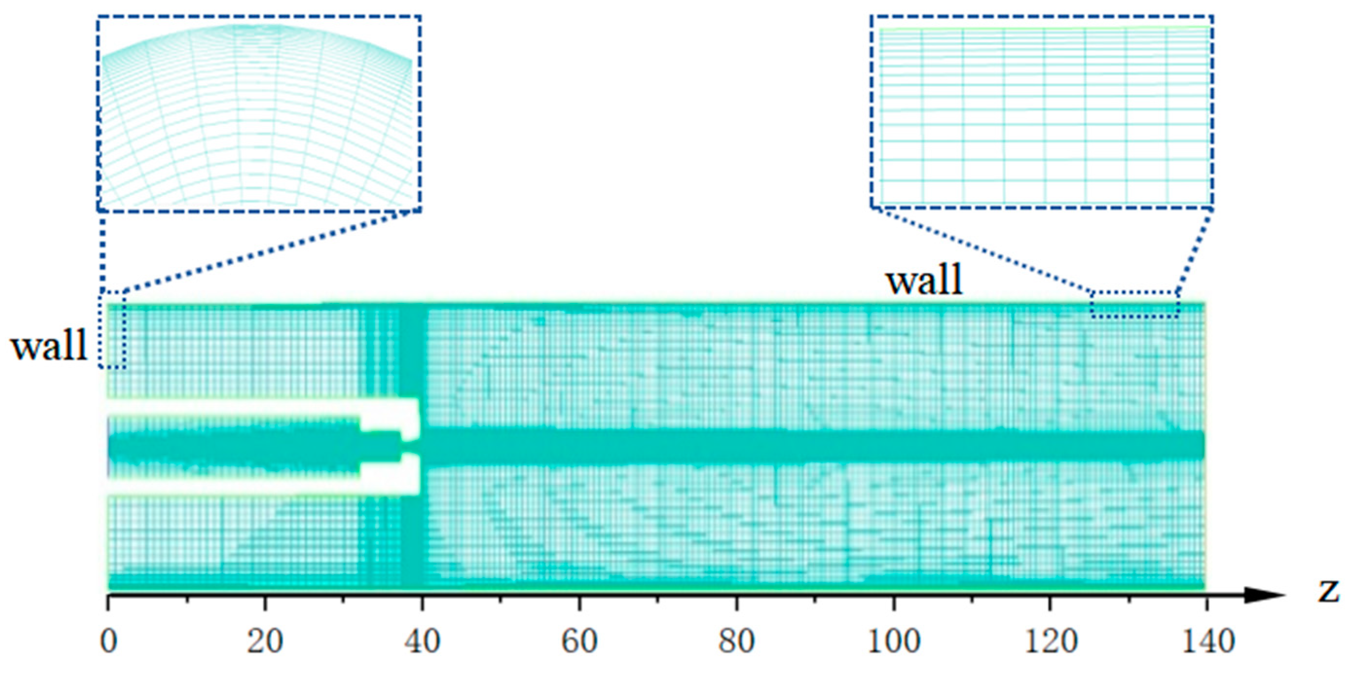
2.2.1. Mesh Generation

The computational boundary must be kept a long way from the nozzle exit in order to reduce the impact of entrainment and reverse the exit flow on the core area of the jet. The literature suggests that the breadth of the computational domain should be more than 100 times the diameter of the nozzle throat. For the fluid computational domain in this investigation, a cylinder with dimensions of 100 mm in length and 30 mm in diameter was chosen, as shown in Figure 2. According to Yun et al. [24], the expected velocity distribution of the improved mesh computation and the experimental results of the cavitation pattern are more consistent. A hexahedral mesh is used to geometrically mesh the flow model in the ICEM program. To make the simulation results better reflect the real cavitation effect, it is necessary to encrypt the mesh of the shear layer and the mesh of the center region of the jet, as shown in Figure 3.

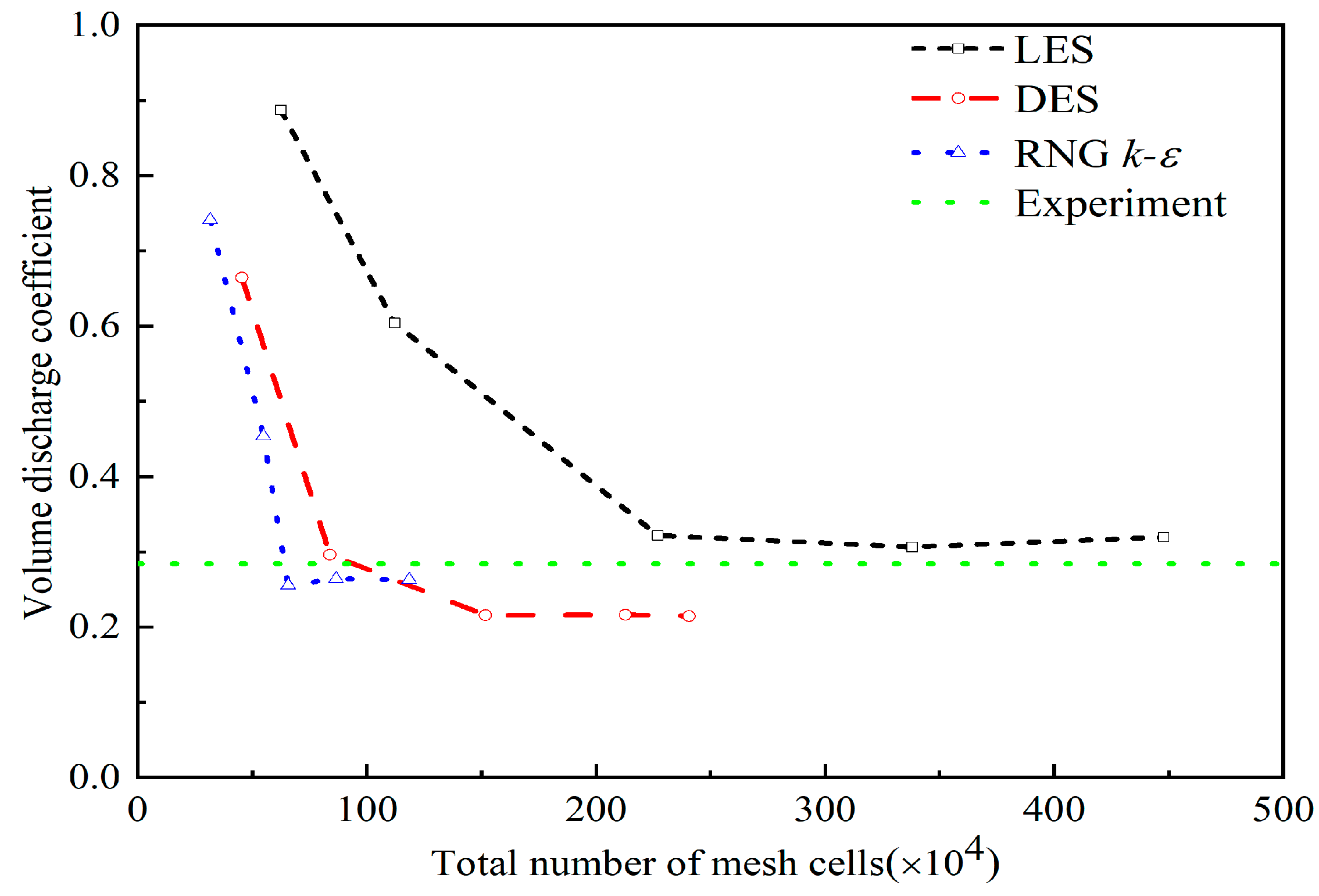
2.2.2. Mesh Independence and Numerical Uncertainty Analysis

The volume discharge coefficient ($C_Q$), which is a useful tool for confirming mesh independence and quantifying uncertainty in numerical simulations, is defined as follows [25]:

$$C_Q=\frac{q_{eff}}{q_{ideal}}$$

(1)

The ideal flow rate through the nozzle derived from the Bernoulli equation is as follows:

$$q_{ideal}=A\sqrt{\frac{2\left(P_1-P_2\right)}{\rho }}$$

(2)

where $A$ is the area of the cross-section, $P_1$ is the inlet pressure, and $P_2$ is the outlet pressure.

The effective flow rate predicted via the simulation is calculated using the following integral equation:

$$q_{eff}={\displaystyle \underset{0}{\overset{\mathrm{R}}{\int }}2\pi \mathrm{r}u\left(r,z\right)}dr$$

(3)

where $r$ is the radial position and $u$ is the local axial velocity at the throat exit of the nozzle.

Figure 4 shows how the volume discharge coefficient changes when the total number of mesh cells rises from 0.307 to 4.636 million. Two fine grids, one medium grid, and two coarse grids make up the array. As the total grid count increases from the first coarse grid to the second coarse grid, the coefficient value ($C_Q$) rapidly decreases. The error value between the middle grid and the second fine grid is less than 2%. Therefore, the number of grid nodes calculated using the RNG k−ε, the DES, the LES models is 0.652, 1.529, and 2.389 million, respectively. A comparison with the experiment reveals that the volume discharge coefficient ($C_Q$) demonstrates a consistent trend of stabilization and converges towards the experimental value as the number of grids increases.

For the grid convergence study, we analyzed the evolution of the mean pressure along the centerline of the jet outlet. Figure 5 illustrates the relationship between the mean pressure along the jet centerline and that for the three models. It is evident from the figure that the mean pressure of the jet at the nozzle exit exhibits greater variability with lower mesh numbers. However, as the mesh number increases, the mean pressure tends to stabilize within the range of the medium grid number and the fine grid number, with a maximum error of less than 5%. Furthermore, while comparing the LES model with the other two models, it is observed that the mean pressures of the latter are consistently smooth inside the cavitation flow field. However, the LES model exhibits a zigzag pattern, which can be attributed to the presence of the cavitation cloud.

2.3. Boundary Conditions and Discretization Methods

The calculations have been carried out while applying ANSYS FLUENT 2021R2 software. The inlet and the outlet are to the pressure boundaries to simulate a 3D flow field with P_in = 7 MPa and P_out = 101.325 kPa. The turbulence intensity is 5%. The inlet and outlet’s hydraulic diameter is 6.4 mm and 30 mm, respectively. The wall boundary condition is used as a no-slip boundary condition. The flow medium is T = 25 °C water with a saturated vapor pressure of 3169 Pa, and the density and viscosity of water is 1000 kg/m³ and 0.89 mPa.s. In this investigation, the onset of cavitation is observed to take place near the nozzle throat, so a Reynolds number of Re = 1.2 × 10⁵ is in this particular area.

For LES with the WALE model, a steady initial flow field is calculated using the SST $k-\omega$ model; the results may then be utilized as the initial flow field. The convergence of the simulation is directly linked to the stability of the flow field in the nozzle exit. In the present investigation, the value of y+ is around 0.479 near the outlet wall of the nozzle.

Table 2. Discrete scheme and accuracy.

Turbulent Model	RNG k−ε Model	LES with WALE Model	DES Model
The coupled pressure–velocity method	Coupled	Coupled	Coupled
The interpolation method with gradient	Least squares cell-based	Least squares cell-based	Least squares cell-based
The interpolation method with pressure	PRESTO!	PRESTO!	PRESTO!
Convection interpolation	2nd-order upwind	Bounded central differencing	Bounded central differencing
Volume fraction interpolation	1st-order upwind	1st-order upwind	1st-order upwind
Time step	1 × 10−5	1 × 10−5	1 × 10−5
Convergence precision	1 × 10−4	1 × 10−4	1 × 10−4
Transient Formulation	Bounded Second-OrderImplicit	First-OrderImplicit	First-OrderImplicit
The Thermal	25 °C	25 °C	25 °C

displays the particular discrete scheme and methodology.

2.4. Control Equations of Mixture Model

A cavitating water jet exhibits characteristics of a vapor–liquid two-phase flow. In order to calculate the flow field, one can opt for either the Euler–Euler or Euler–Lagrangian method. The Euler–Euler technique is frequently used to compute two-phase flows when the motion of the discrete phases is ignored. In this work, the vapor–liquid two-phases flow is simulated using the mixture model based on the Euler–Euler technique.

2.4.1. Continuity Equation

The following is the method to formulate the continuity equation for mixtures [26]:

$$\frac{\partial }{\partial t}\left({\rho }_m\right)+\nabla \cdot \left({\rho }_m{\overrightarrow{v}}_m\right)=0$$

(4)

where ${\overrightarrow{v}}_m$ is the mass-averaged velocity,

$${\overrightarrow{v}}_m=\frac{{\displaystyle \sum _{k=1}^n{\alpha }_k{\rho }_k{\overrightarrow{v}}_k}}{{\rho }_m}$$

(5)

and ${\rho }_m$ is the mixture density,

$${\rho }_m={\displaystyle \sum _{k=1}^n{\alpha }_k{\rho }_k}$$

(6)

while ${\alpha }_k$ represents the volume fraction of phase k.

2.4.2. Momentum Equation

By combining the momentum equations for the gas phase and the liquid phase, the momentum equation for the mixture can be created, which has the following form [27]:

$$\begin{array}{ll}\frac{\partial }{\partial t}\left({\rho }_m{\overrightarrow{v}}_m\right)+\nabla \cdot \left({\rho }_m{\overrightarrow{v}}_m{\overrightarrow{v}}_m\right)& =-\nabla p+\nabla \cdot \left[{\mu }_m\left(\nabla {\overrightarrow{v}}_m+\nabla {\overrightarrow{v}}_m^T\right)\right]\\ & +{\rho }_m\overrightarrow{g}+\overrightarrow{F}-\nabla \cdot \left({\displaystyle \sum _{k=1}^n{\alpha }_k{\rho }_k{\overrightarrow{v}}_{dr,k}{\overrightarrow{v}}_{dr,k}}\right)\end{array}$$

(7)

where n is the number of phases; when simulating the cavitating jets numerically, water and water vapor make up the flow medium, so n = 2. $\overrightarrow{F}$ is defined as a body force, and the effect of the volume forces is ignored here. ${\mu }_m$ is defined as the viscosity of mixtures:

$${\mu }_m={\displaystyle \sum _{k=1}^n{\alpha }_k{\mu }_k}$$

(8)

and ${\overrightarrow{v}}_{dr,k}$ is for the slipping velocity of phase k:

$${\overrightarrow{v}}_{dr,k}={\overrightarrow{v}}_k-{\overrightarrow{v}}_m$$

(9)

2.5. Zwart–Gerber–Belamri (ZGB) Cavitating Model

The vapor–liquid mass transfer is computed using the mixture model, which is used to calculate the two-phase cavitating flow.

$$\frac{\partial }{\partial t}\left(\alpha {\rho }_v\right)+\nabla \cdot \left(\alpha {\rho }_v{\overrightarrow{v}}_v\right)=R_e-R_c$$

(10)

In this equation, the subscript v stands for the vapor phase, while $\alpha$ indicates the vapor phase’s volume fraction. The source terms for the mass transfer associated with the formation and deflation of the cavitation bubbles are $R_e$ and $R_c$, respectively. A Rayleigh–Plesset equation may be employed to calculate them [28]. The mass transition between the phases of water and vapor has been calculated using the ZGB cavitating model, as shown below:

$$\mathrm{If}P\le P_v{R}_e=F_{vap}\frac{3{\alpha }_{nuc}\left(1-{\alpha }_v\right){\rho }_v}{{\Re }_B}\sqrt{\frac{2}{3}\frac{P_v-P}{{\rho }_l}}$$

(11)

$$\mathrm{If}P\ge P_v\mathrm{C}{R}_c=F_{cond}\frac{3{\alpha }_v{\rho }_v}{{\Re }_B}\sqrt{\frac{2}{3}\frac{P-P_v}{{\rho }_l}}$$

(12)

where, $P$ stands for the local far-field pressure, $P_v$ stands for the saturation vapor pressure, ${\Re }_B={10}^{-6}m$ stands for the bubble radius, ${\alpha }_{nuc}=5\times {10}^{-4}$ stands for the volume fraction of the nucleation site, $F_{vap}=0.02$ stands for the evaporation coefficient, $F_{cond}=0.01$ stands for condensation coefficient, and ${\rho }_l$ stands for the density of the liquid phase.

Equation (10) is used to model the threshold pressure taking into account the effects of turbulence. The threshold pressure is calculated from

$$P_v=P_{sat}+\frac{1}{2}c{\rho }_l{k}_l$$

(13)

where, $P_{sat}$ represents the saturation pressure, $k_l$ represents the turbulent kinetic energy of the liquid phase, and the recommended value of the constant, $c$, is 0.39.

2.6. Turbulent Model

For closing the continuity and momentum equations, the different turbulent models are proposed. Here, the flow around the cavitating nozzle of the organ pipe is modeled using the RNG k−ε, LES, and DES models, and the impact of these three cavitation models on the numerical calculation of the cavitation water jet is evaluated [29].

2.6.1. RNG k−ε Model

The time-average theories served as the foundation for the RNG k−ε model. It has better accuracy and reliability for a wider range of flows. The turbulence control equations are as follows:

$$\frac{\partial }{\partial t}\left(\rho k\right)+\frac{\partial }{\partial x_i}\left(\rho k{u}_i\right)=\frac{\partial }{\partial x_j}\left({\alpha }_k{\mu }_{eff}\frac{\partial k}{\partial x_j}\right)+G_k-\rho \epsilon$$

(14)

$$\frac{\partial }{\partial t}\left(\rho \epsilon \right)+\frac{\partial }{\partial x_i}\left(\rho \epsilon u_i\right)=\frac{\partial }{\partial x_j}\left({\alpha }_{\epsilon }{\mu }_{eff}\frac{\partial \epsilon }{\partial x_j}\right)+C_{1\epsilon }\frac{\epsilon }{k}\left(G_k+C_{3\epsilon }{G}_b\right)-C_{2\epsilon }\rho \frac{{\epsilon }^2}{k}-R_{\epsilon }$$

(15)

where, G_k is the turbulence kinetic energy generated via the mean velocity gradients, and α_k and α_ε represent the Prandtl numbers. The constants of C_1ε, C_2ε and C_3ε are detailed in the literature.

2.6.2. LES with the WALE Model

The LES equations are acquired by filtering the time-dependent N-S equations. The sub-grid-scale (SGS) model is used to simulate the small-scale turbulence, whereas the large-scale turbulence is estimated explicitly [25,30]. Therefore, the LES model has a higher computational cost than does the RANS model. The sub-grid-scale turbulent stresses can be calculated as follows:

$${\tau }_{ij}=-2{\mu }_t{\overline{S}}_{ij}+\frac{1}{3}{\tau }_{kk}{\delta }_{ij}$$

(16)

where ${\mu }_t$ represents the SGS turbulent viscosity, and ${\overline{S}}_{ij}$ represents the strain tensor rate at the resolved scale. To compute the cavitating flow, a sub-grid model using the WALE (wall-adapting local eddy-viscosity) model is used. The eddy viscosity was determined using the WALE model, whereby

$${\mu }_t=\rho L_s^2\frac{{\left(S_{ij}^d{S}_{ij}^d\right)}^{\frac{3}{2}}}{{\left({\overline{S}}_{ij}{\overline{S}}_{ij}\right)}^{\frac{5}{2}}+{\left(S_{ij}^d{S}_{ij}^d\right)}^{\frac{5}{4}}}$$

(17)

In this model, $L_s$ and $S_{ij}^d$ are taken by the following equations:

$$L_s=\min \left(Kd,C_w{V}^{\frac{1}{3}}\right)$$

(18)

$$S_{ij}^d=\frac{1}{2}\left({\overline{g}}_{ij}^2+{\overline{g}}_{ji}^2\right)-\frac{1}{3}{\delta }_{ij}{\overline{g}}_{kk}^2,{\overline{g}}_{ij}=\frac{\partial {\overline{u}}_i}{\partial x_j}$$

(19)

where K is the Carmen constant, d denotes the distance from the wall, V denotes the volume of mesh, and $C_w$ = 0.325 denotes the WALE model constant.

2.6.3. DES with the SST k−ω Model

The RANS model was unable to achieve the necessary accuracy. The LES model’s use has been constrained by high calculation costs. In recent years, there has been an increase in interest in the RANS–LES hybrid model. When the DES approach was utilized, the near-wall zone was calculated using the RANS model, and the turbulent separated zone was computed using the LES model. The fully formed turbulent zone, where the flow is mostly large-scale unstable turbulence, is the calculation zone for the LES model.

The control equations of the DES model with the SST model [31] are as follows:

$$\frac{\partial }{\partial t}(\rho k)+\frac{\partial }{\partial x_i}\left(\rho k{u}_i\right)=\frac{\partial }{\partial x_j}\left({\Gamma }_k\frac{\partial k}{\partial x_j}\right)+G_k-Y_k+S_k$$

(20)

$$\frac{\partial }{\partial t}(\rho \omega )+\frac{\partial }{\partial x_i}\left(\rho \omega u_i\right)=\frac{\partial }{\partial x_j}\left({\Gamma }_{\omega }\frac{\partial \omega }{\partial x_j}\right)+G_{\omega }-Y_{\omega }+S_{\omega }$$

(21)

$G_{\omega }$ represents the generation of $\omega$. The symbols ${\Gamma }_k$ and ${\Gamma }_{\omega }$ are used to denote the effective diffusivity of substances $k$ and $\omega$, respectively. The variables $Y_k$ and $Y_{\omega }$ are used to denote the dissipation of energy and the dissipation of momentum caused by turbulence, respectively. $S_k$ and $S_{\omega }$ represent the source term.

$$Y_k=\rho {\beta }^{*}k\omega F_{DES}$$

(22)

$${\beta }^{*}={\beta }_i^{*}\left[1+{\zeta }^{*}F\left(M_t\right)\right]$$

(23)

$${\beta }_i^{*}={\beta }_{\infty }^{*}\left(\frac{4/15+{\left(R{e}_t/R_{\beta }\right)}^4}{1+\left(R{e}_t/R_{\beta }\right)}\right)$$

(24)

$$R{e}_t=\frac{\rho k}{\mu \omega }$$

(25)

where ${\zeta }^{*}=1.5$,$R_{\beta }=8$, ${\beta }_{\infty }^{*}=0.09$, $\omega$ is the specific dissipation rate.

$F_{DES}$ is expressed as follows:

$$F_{DES}=\max \left(\frac{L_t}{C_{des}{\Delta }_{\max }}\left(1-F_{SST}\right),1\right)$$

(26)

where $C_{des}=0.61$ is the constant, ${\Delta }_{\max }$ is the grid spacing, $F_{SST}=0,F_1,F_2$, $F_1$ and $F_2$ represent the hybrid functions. $L_t$ represents the parameter of the turbulent length scale as follows:

$$L_t=\frac{\sqrt{k}}{{\beta }^{*}\omega }$$

(27)

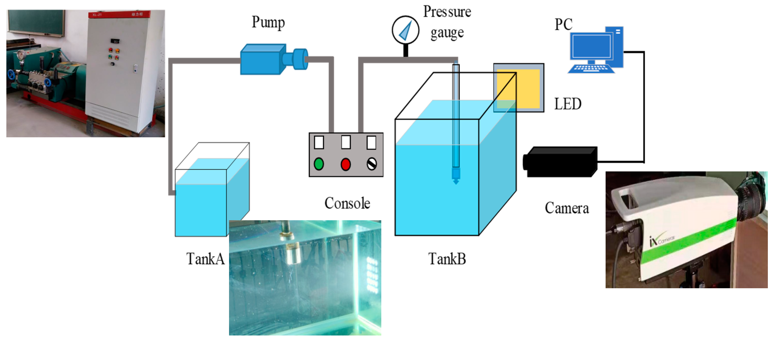
3. Experimental Methods

According to the above-simulated organ pipe nozzle, this study establishes a flow field test apparatus to test the flow field of a submerged cavitating jet. The test apparatus is shown in Figure 6; a high-pressure piston pump (3DY6000/28) was used with a rated flow rate of 6000 L/h and a rated pressure of 28 MPa. A pressure gauge (DYLY-102) was used to measure the pressure, in a range of 0–30 MPa and with an error of ±0.3 FS. The water tank was subjected to the injection of high-pressure water via the organ pipe nozzle. The water tank was constructed using acrylic resin material, which effectively mitigated light refraction and thereby guaranteed the precision of high-speed photography. The camera module comprised an LED light source and an Olympus high-speed camera, model X18-2-4, equipped with a CH-S400 camera lens. The high-speed camera shot at 10,000 fps with a time interval of 0.1 ms between every two photos, and a shooting size of 528 pixels × 400 pixels. The upstream pressure was adopted as 7 MPa, and the corresponding cavitation number [23] was 0.0144.

4. Results and Discussion

4.1. Comparison of the Simulation and Experiments Results

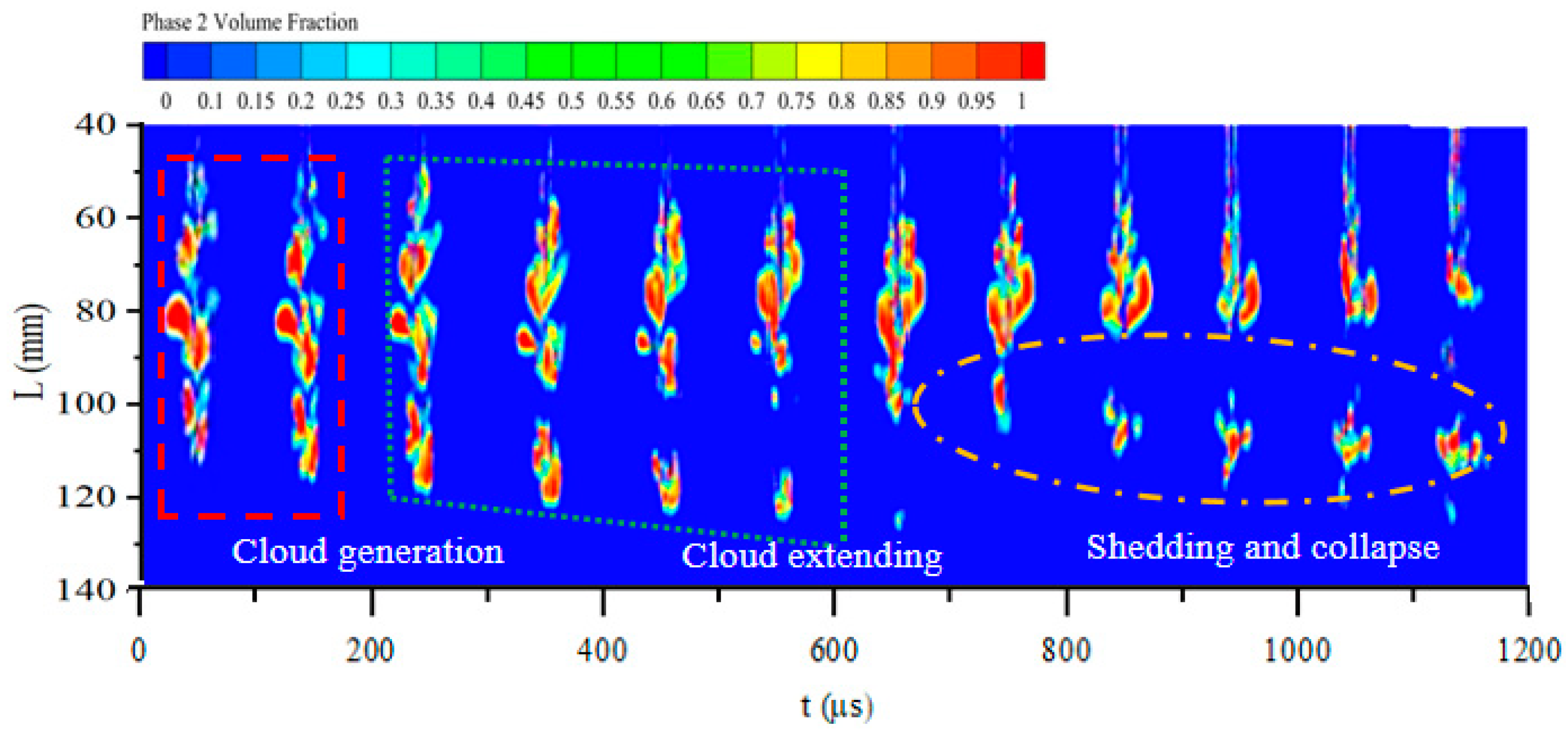
4.1.1. LES Simulation Results for Cavitating Cloud Evolution

The numerical findings pertaining to the phenomenon of a cavitating water jet are further examined in relation to the experimental data. The experimental investigation focused on the study of cavitation at a Reynolds number of Re = 1.2 × 10⁵, accompanied by a cavitation number (σ) of 0.0144. The average temperature observed in the experiment was approximately 25 °C, which closely aligned with the simulated parameters. Figure 7 and Figure 8 present a comparison between the numerical results and a series of high-speed photographic images derived from the experimental data.

Given the limitations of the RNG k−ε and DES models in accurately simulating the cavitation cloud at the nozzle exit, the LES model is employed to simulate the spatial and temporal evolution of the cavitation cloud, as depicted in Figure 7. The depicted region characterized by a larger vapor-phase volume fraction (indicated by the color red) in the figure signifies the occurrence and progression of cavitation cloud formation. The cavitating cloud images are saved every 10 time steps, which means that these are saved every 100 µs. The results show that the development period of cavitation is about 1200 µs. The cavitating clouds first generate at t = 0–200 µs, develop at t = 200–600 µs, shed at t = 600–900 µs, and then collapse at t = 900–1200 µs.

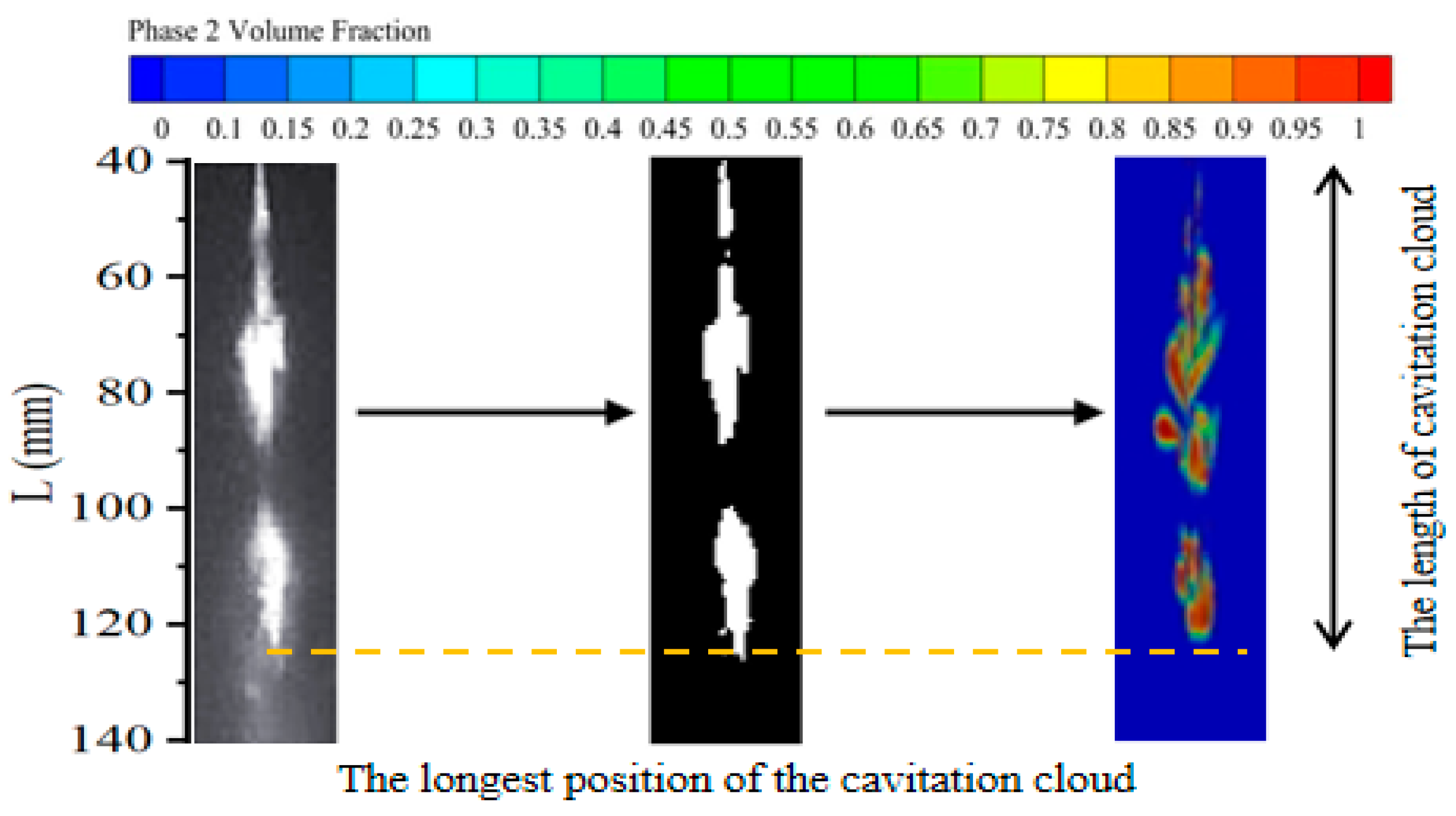
4.1.2. The Experiment Results

Figure 8 illustrates the cavitation cloud images produced through the use of experimental pictures. The results of the cavitation cloud evolution experiments show that the LES calculations are in good agreement with the experimental data, indicating that the LES turbulence model is suitable for the simulation and prediction of the cavitation cloud process. Although the obtained flow field images may not show the same circulation patterns as the experimental results do, they can still describe the whole process of cavitation cloud shedding, from growth to collapse. In addition, there are slight differences in the comparison between the experimental and simulation results. For example, in the experiments, some small cloud cavities collapse and extend downstream of the filamentary cavitation. However, numerical simulations do not anticipate these events. The cavitation cloud images captured with the high-speed camera were transformed into binary images and subsequently compared to the simulation results, as depicted in Figure 9. After the cavitation cloud reached full development, its maximum length measured approximately 90 mm, aligning closely with the outcomes of the simulation.

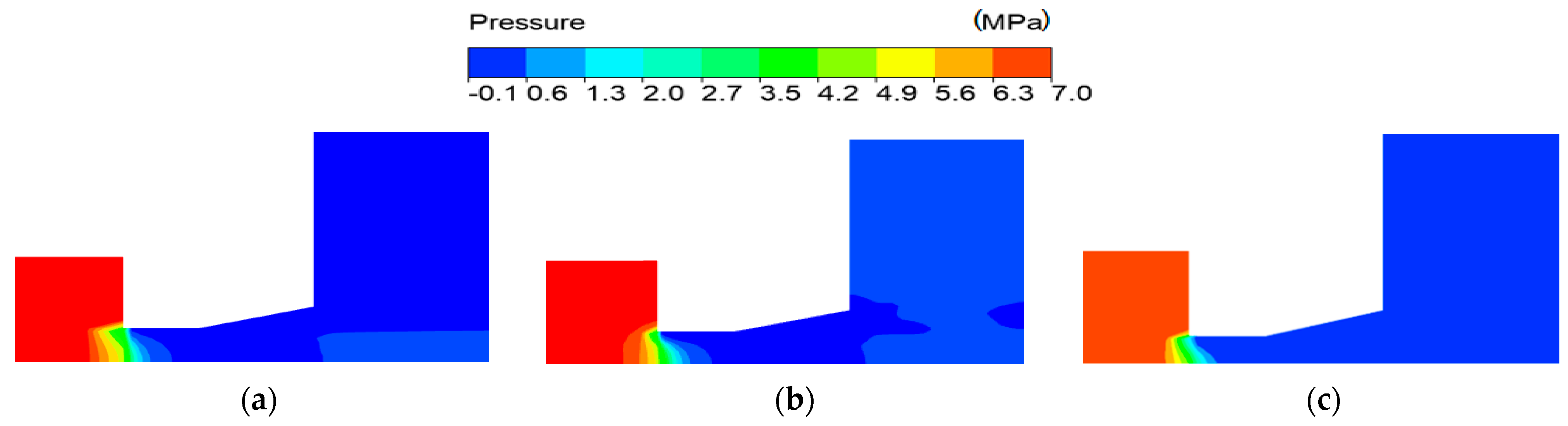
4.2. The Cavitating Jet Flow Field with Different Turbulence Models

Figure 10 displays the static pressure computed utilizing the RNG k−ε, DES, and LES models. We can see from the figure that the static pressure cloud images of three models are not significantly different. The static pressure rapidly reduces in the cylindrical and diffusion section, and negative pressure is generated. The cavitation process initiates as the pressure at a given location falls below the saturation vapor pressure, resulting in the transformation of liquid water into vapor.

Figure 11 depicts the velocity streamline distributions for the three turbulence models. As depicted in figure, the fluid demonstrates a rapid flow within the cylindrical segment, while flow separation is observed within the diffusive segment. The LES model calculations show that a significant vortex ring is generated in the nozzle throat region, which is a typical phenomenon of cavitation formation.

Figure 12 illustrates the vapor-phase volume fraction for the three turbulence models. Cavitation is generated at the location of the separation and vortex ring. Based on the findings of Ferrari [32], the efficiency of cavitation generation is influenced by the intensity of the vortex ring when the static pressure falls below the saturation vapor pressure. The geometric configuration of the nozzle undergoes alterations in both the cylindrical and diffusion sections. When the fluid flows from the cylindrical section into the diffusion section, there is an obvious expanding diameter where there is an interaction between the fluid and the wall, which promotes the growth of vortex rings, and accelerates the cavitation.

The area of cavitation calculated with the LES model is the maximum among the three simulation results as shown in Figure 12. Therefore, the vortex rings and the cavitation effects were successfully simulated using the LES model. Furthermore, when comparing the RNG k−ε model with the DES model, it is observed that the DES model is capable of simulating a larger separated flow area. Additionally, the DES model exhibits superior performance in simulating cavitation intensity compared to that of the RNG k−ε model.

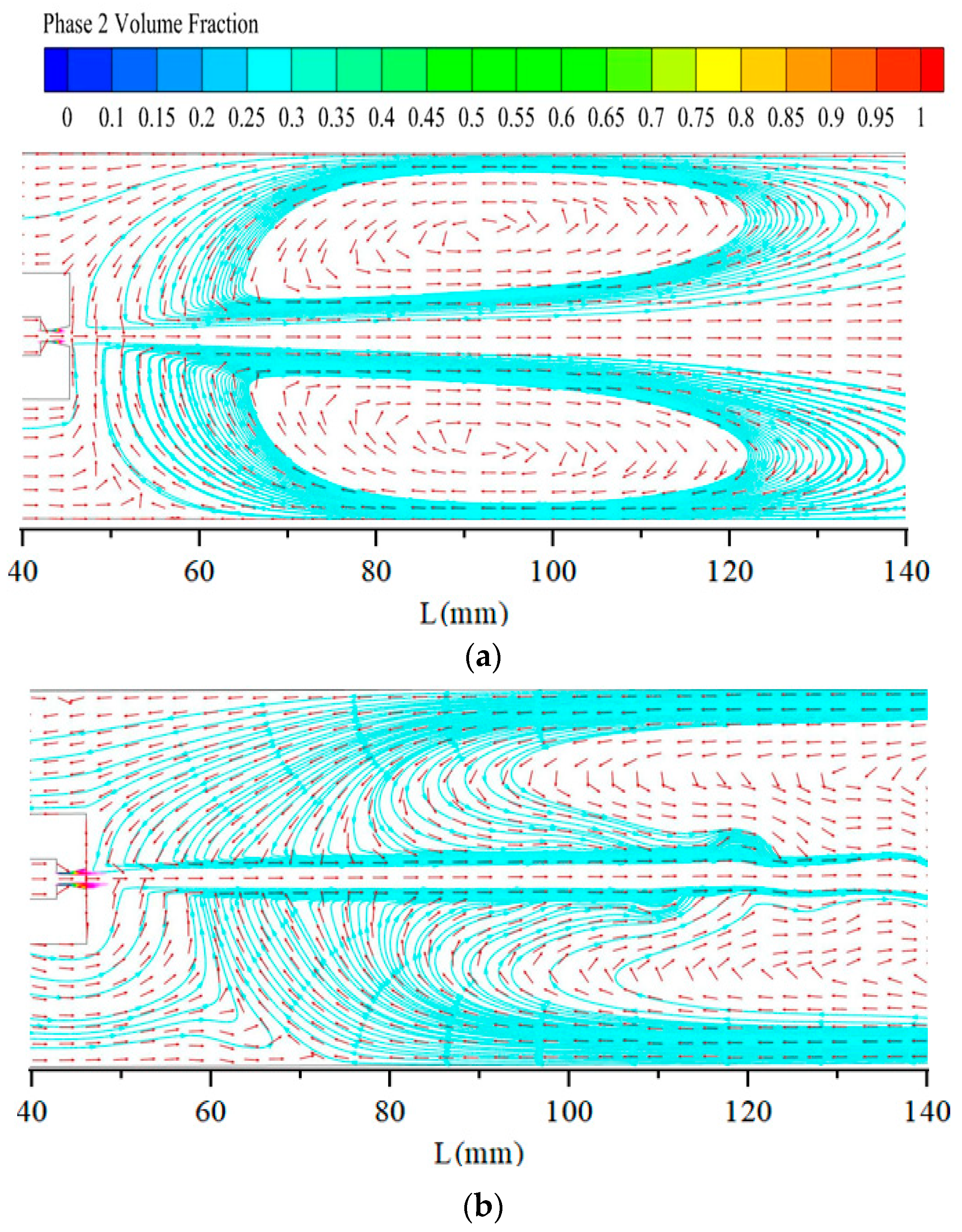
4.3. The Flow Field Outside Nozzles with Different Turbulence Models

The analysis of the cavitating mechanism involved studying the flow field outside the nozzles. Figure 13 depicts the velocity streamlines observed in the vicinity of nozzles employing various turbulent models. The cloud image depicted in the velocity streamlines corresponds to the volumetric proportion of the vapor phase. The presence of vortex structures of varying scales can be observed in the velocity streamlines on both sides of the jet flow. The simulation results calculated using the LES model show more small-scale vortexes, and re-entrant jets were formed outside the nozzle; this is where the cavitation cloud produced periodic collapses. However, it is difficult to determine the precise location of the re-entrant jet, which is more likely to be in the cavity closure position. Then, the simulation results of the two other turbulence models show the two relatively symmetrical large-scale vortexes, and no obvious cavitating clouds was generated outside the nozzle.

The velocity vector at the outlet of the diffusion section (Z = 40 mm) is shown in Figure 14a. The simulation results obtained using the RNG k−ε model indicate that there is minimal radial flow generated. Instead, the fluid predominantly flows in the direction of the jet, as depicted in Figure 14(a1). According to the DES simulation results, the large-scale eddies’ current and the fluid flow are relatively stable as shown in Figure 14(a2). The LES simulation results show that the cavitating cloud appears early at the Z = 40 mm section. The jet interacts with the stationary fluid, the large pressure gradient is generated and the strong shearing effect drives the development of the vortex rings. It can be seen from Figure 14(a3), that there are four symmetric vortex rings.

Figure 14b highlights the velocity vector in the section where Z = 60 mm. The simulation outcomes obtained using the RNG k−ε and DES models demonstrate a reduction in high-velocity regions, indicating a relatively stable jet flow. This observation is depicted in Figure 14(b1,b2). According to the LES results, the cavitating clouds develop further as shown in Figure 14(b3). The flow’s instability is further enhanced in this section and the complex vortexes present around the center of the jet.

Figure 14c indicates the velocity vector in the Z = 80 mm section. The reduction in the core region of the jet and the decrease in the shearing effect can be observed in the simulation results that utilize the RNG k−ε and DES models, as depicted in Figure 14(c1,c2). The LES simulation results show the annular vortex structure from inside to outside, which means that the cavitation cloud flows down as shown in Figure 14(c3). While the cavitating clouds develop to their maximum and shed from the main body of the cavitating cloud, the typical vortex rings no longer appear and the jet flow is accompanied by large-scale vortexes.

Figure 14d represents the velocity vector in the section where Z = 100 mm. The simulation results of the RNG k−ε model indicate that the flow remains largely unaltered, as depicted in Figure 14(d1). The simulation results of the DES model, as depicted in Figure 14(d2), illustrate the presence of a significant vortex structure in the flow. According to the LES results, the cavitation bubbles begin to collapse here as shown in Figure 14(d3). When the cavitation bubbles collapse, strong turbulence is induced and the fluctuation of the flow field is enhanced. The velocities further decrease and unsymmetrical vortexes grow in this section.

In order to further study the simulation effect of the three turbulence models on cavitation, as the vapor volume fraction of the cavitating cloud outside the nozzles varied periodically, the cavitating clouds were time-averaged over 5 time periods to compare the variation in different turbulence models. The volume fraction of the vapor phase with different turbulent models is shown in Figure 15. The results calculated using RNG k−ε model and DES model show that cavitation is generated only in the diffusion section of the nozzle, and no cavitation cloud is generated outside the nozzle. However, the LES model can simulate well the periodic evolution of the cavitation cloud outside the nozzle.

The Q-criteria of vorticity was used to identify the vortex structure in accordance with $Q=5.0\times {10}^5 {\mathrm{s}}^{-2}$ [33]. Figure 16 demonstrates the progression of the vortex structure over time, here colored by velocity. The results simulated using the RNG k−ε model and DES model show that there is no obvious periodicity for the vorticity evolutions, and the morphology of vorticity at different times is basically the same as that depicted in Figure 16a,b. The LES simulation results show that the cavitating cloud presents a periodic evolution and a vortex structure exists during the generation, development, shedding and collapse stages, respectively, as shown in Figure 16c. During the cavitating cloud’s generation, the vortex is small and its front end moves forward; during the cavitating cloud’s development, the vortex structure further increases and its radial size increases significantly compared to that in the previous stage. During the cavitating cloud’s shedding, the vortexes continues to move forward and the front end of the vortexes start to become smaller with no significant change in radial size. During the cavitating cloud’s collapse, the cavitation bubbles collapse, and the fluid is disturbed, which makes the large vortexes break up into small vortexes.

5. Conclusions

(1)

The numerical simulation of the cavitating flow in the organ pipe nozzle was conducted using the mixture model, the ZGB cavitation model, and three turbulence models, namely the RNG k−ε, DES, and LES models. The findings from three turbulence models indicate that the static pressure in both the cylindrical and diffusion sections is below the saturation vapor pressure of water. The velocity streamlines of the RNG k−ε and DES models exhibit a separation flow, whereas the velocity streamlines of the LES model demonstrate the presence of vortex rings in close proximity to the cylindrical and diffusion sections. These vortex rings contribute to the formation of cavitation. The LES model demonstrates effective simulation capabilities for accurately representing the cavitating flow phenomena in an organ pipe nozzle.

(2)

The cavitating cloud evolutions of an organ pipe nozzle were achieved using high-speed photography. There were periodic developments: the generation, development, shedding and collapse stages for cavitating clouds. The development period of a cavitating cloud is about 1200 µs and the maximum length of a cavitating cloud is about 90 mm at the inlet pressure of 7 MPa. The RNG k−ε and DES models are inadequate in simulating the formation of cavitation clouds outside the nozzle. In contrast, the LES model is capable of accurately simulating the dynamic behavior of cavitating clouds, which aligns well with experimental observations.

(3)

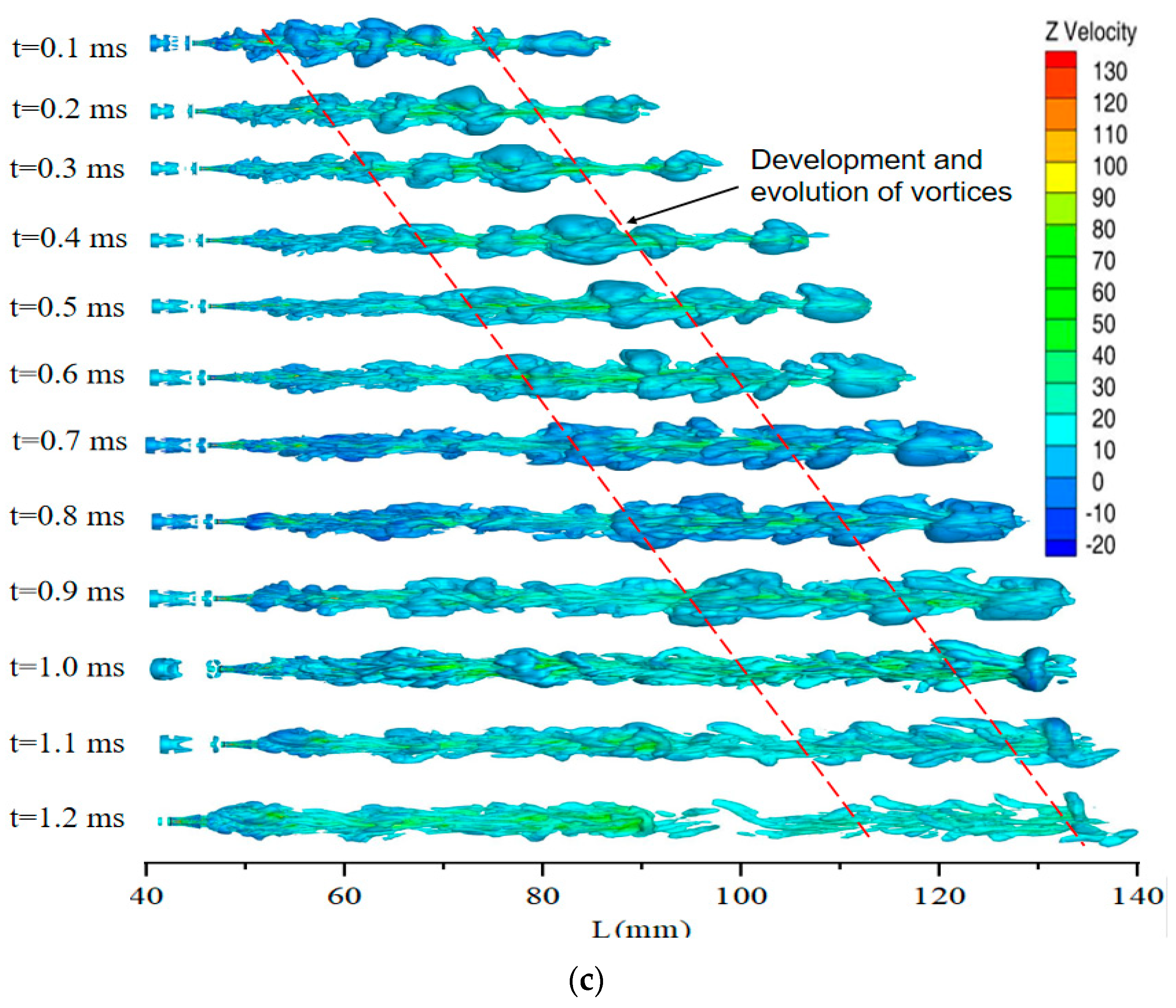
The LES model accurately replicates the evolution of vorticity, which exhibits a consistent pattern during the periodic formation of a cavitation cloud. The dimensions of the vortex structure expand as the cavitating jet progresses, and the asymmetrical vortexes in the cross-sectional area experience growth during the initial stages of the cavitation jet. The cavitation bubble’s collapse at the termination of the cavitation jet induces perturbations in the adjacent fluid, causing the fragmentation of macroscopic vortexes into smaller-scale vortexes.

References

1. Ge, M.M.; Petkovšek, M.; Zhang, G.J.; Jacobs, D.; Coutier-Delgosha, O. Cavitation dynamics and thermodynamic effects at elevated temperatures in a small Venturi channel. Int. J. Heat Mass Transf. 2021, 170, 120970. [Google Scholar] [CrossRef]
2. Soyama, H. Cavitating Jet: A Review. Appl. Sci. 2020, 10, 7280. [Google Scholar] [CrossRef]
3. Li, G.S.; Liao, H.L.; Huang, Z.W.; Shen, L.H. Rock Damage Mechanisms under Ultra-high Pressure Water Jet Impact. J. Mech. Eng. 2009, 45, 284–293. [Google Scholar] [CrossRef]
4. Cai, S.G.; Liu, P.T.; Zhao, X.J.; Chen, C.H.; Ren, R.M. Water Cavitation Peening-induced Surface Hardening and Cavitation Damage of Pure Titanium. China Surf. Eng. 2014, 27, 100–105. [Google Scholar]
5. Shi, F.X.; Zhao, J.; Sun, X.G.; Yin, H.L. Numerical Simulation of Surface Cleaning Flow Field by Gas-Liquid Two-Phase Jet. J. Cent. South Univ. (Nat. Sci. Ed.) 2021, 52, 960–970. [Google Scholar]
6. Szolcek, M.; Cassineri, S.; Cioncolini, A.; Scenini, F.; Curioni, M. CRUD Removal via Hydrodynamic Cavitation in Micro-Orifices. Nucl. Eng. Des. 2019, 343, 210–217. [Google Scholar] [CrossRef]
7. Ge, M.M.; Sun, C.Y.; Zhang, G.J. Olivier Coutier-Delgosha, Dixia Fan, Combined suppression effects on hydrodynamic cavitation performance in Venturi-type reactor for process intensification. Ultrason. Sonochem. 2022, 86, 106035. [Google Scholar] [CrossRef]
8. Han, J.; Cai, T.F.; Pan, Y.; Ma, F. Study on Jet’ s Characteristics of Organ Nozzle and Helmholtz Nozzle. Saf. Coal Mine 2017, 48, 134–137. [Google Scholar]
9. Wang, C.H.; Hu, Y.N.; Rao, C.J.; Deng, X.G. Numerical Analysis of Cavitation Effects and Self-excited Oscillation Pulse Nozzle and Jet Forms. China Mech. Eng. 2017, 28, 1535–1541. [Google Scholar]
10. Yu, H.T.; Xu, Y.; Wang, J.Y.; Liu, H.S.; Zhang, J.L.; Wang, Z.C. Optimization of Organ Pipe Nozzle Structure Based on CFD. Chem. Eng. Mach. 2021, 48, 883–887. [Google Scholar]
11. Cai, T.F.; Pan, Y.; Ma, F.; Qiu, L.B.; Xu, P.P. Effects of Outlet Geometry of Organ-pipe Nozzle on Cavitation Due to Impingement of the Waterjet. J. Mech. Eng. 2019, 55, 150–156. [Google Scholar]
12. Dong, W.; Yao, L.; Luo, W. Numerical Simulation of Flow Field of Submerged Angular Cavitation Nozzle. Appl. Sci. 2023, 13, 613. [Google Scholar] [CrossRef]
13. Ran, Z.; Ma, W.; Liu, C. 3D Cavitation Shedding Dynamics: Cavitation Flow-Fluid Vortex Formation Interaction in a Hydrodynamic Torque Converter. Appl. Sci. 2021, 11, 2798. [Google Scholar] [CrossRef]
14. Yan, C.Y.; Chen, Y. Numerical Investigation on the Water-Entry Cavity Feature and Flow Structure of a Spinning Sphere Based on Large-Eddy Simulation. Chin. J. Theor. Appl. Mech. 2022, 54, 1012–1025. [Google Scholar]
15. Cheng, H.Y.; Ji, B.; Long, X.P.; Huai, W.X. LES Invetigation on The Influence of Cavitation on The Evolution and Characteristics of Tip Leakage Vortex. Chin. J. Theor. Appl. Mech. 2021, 53, 1268–1287. [Google Scholar]
16. Xue, M.; Pu, Y. Large Eddy Simulation on Cavitation Inception of A Diesel Nozzle. Eng. Mech. 2013, 30, 417–422. [Google Scholar]
17. Yang, Y.F. Investigation on Mechanism of Submerged High-Pressure Cavitation Jet and Metal Strength Improvement Using Cavitation Bubble Shock Wave; Jiangsu University: Zhenjiang, China, 2020. [Google Scholar]
18. Yang, Y.; Shi, W.D.; Tan, L.W.; Li, W.; Chen, S.P.; Ban, B. Numerical Research of the Submerged High-Pressure Cavitation Water Jet Based on the RANS-LES Hybrid Model. Shock Vib. 2021, 2021, 16718. [Google Scholar] [CrossRef]
19. Wang, G.; Yang, Y.; Wang, C.; Shi, W.; Li, W.; Pan, B. Effect of Nozzle Outlet Shape on Cavitation Behavior of Submerged High-Pressure Jet. Machines 2022, 10, 4. [Google Scholar] [CrossRef]
20. Sou, A.; Biçer, B.; Tomiyama, A. Numerical Simulation of Incipient Cavitation Flow In a Nozzle of Fuel Injector. Comput. Fluids 2014, 103, 42–48. [Google Scholar] [CrossRef]
21. Trummler, T.; Schmidt, S.J.; Adams, N.A. Investigation of Condensation Shocks and Re-entrant Jet Dynamics in a Cavitating Nozzle Flow by Large-Eddy Simulation. Int. J. Multiph. Flow 2020, 125, 103215. [Google Scholar] [CrossRef]
22. Ge, M.M.; Zhang, G.J.; Petkovšek, M.; Long, K.P.; Coutier-Delgosha, O. Intensity and regimes changing of hydrodynamic cavitation considering temperature effects. J. Clean. Prod. 2022, 338, 130470. [Google Scholar] [CrossRef]
23. Xu, Y.; Liu, H.S.; Wang, Z.C.; Zhang, J.L.; Wang, J.X. Analysis of the Efects of Nozzle Geometry on the Cavitation Water Jet Flow Field Using Orthogonal Decomposition. Iran. J. Sci. Technol. Trans. Mech. Eng. 2023. [Google Scholar] [CrossRef]
24. Long, Y.; Long, X.-P.; Ji, B.; Huai, W.-X.; Qian, Z.-D. Verification and validation of URANS simulations of the turbulent cavitating flow around the hydrofoil. J. Hydrodyn. Ser. B 2017, 16, 60774–60776. [Google Scholar] [CrossRef]
25. Han, X.D.; Kang, Y.; Li, D.; Zhao, W.G. Effects of surface roughness on self-excited cavitating water jet intensity in the organ-pipe nozzle: Numerical simulations and experimental results. Mod. Phys. Lett. B 2019, 33, 1950324. [Google Scholar] [CrossRef]
26. Yang, Y.F.; Li, W.; Shi, W.D.; Zhang, W.Q. Numerical Investigation of a High-Pressure Submerged Jet Using a Cavitation Model Considering Effects of Shear. Processes 2019, 7, 541. [Google Scholar] [CrossRef]
27. Tian, C.L.; Chen, T.; Zou, T. Numerical study of unsteady cavitating flows with RANS and DES models. Mod. Phys. Lett. B. Condens. Matter Phys. Stat. Phys. Appl. Phys. 2019, 33, 20. [Google Scholar] [CrossRef]
28. Savchenko, Y.N.; Savchenko, G.Y.; Semenov, Y.A. Effect of a Boundary Layer on Cavity Flow. Mathematics 2020, 8, 909. [Google Scholar] [CrossRef]
29. Launder, B.E.; Spalding, D.B. Lectures in Mathematical Models of Turbulence; Academic Press: London, UK, 1972. [Google Scholar]
30. He, Z.X.; Chen, Y.H.; Leng, X.Y.; Wang, Q.; Guo, G.M. Experimental visualization and LES investigations on cloud cavitation shedding in a rectangular nozzle orifice. Int. Commun. Heat Mass Transf. Rapid Commun. J. 2016, 76, 108–116. [Google Scholar] [CrossRef]
31. Ge, M.M.; Manikkam, P.; Ghossein, J.; Kumar Subramanian, R.; Coutier-Delgosha, O.; Zhang, G.J. Dynamic mode decomposition to classify cavitating flow regimes induced by thermodynamic effects. Energy 2022, 254 Pt C, 124426. [Google Scholar] [CrossRef]
32. Ferrari, A. Fluid Dynamics of Acoustic and Hydrodynamic Cavitation in Hydraulic Power Systems. Proc. R. Soc. A Math. Phys. Eng. Sci. 2017, 473, 20160345. [Google Scholar] [CrossRef]
33. Zhao, B.J.; Xie, J.T.; Liao, W.Y. Applicability Analysis of the Second Generation Vortex Identification Method in the Internal Flow Field of Mixed-Flow Pump. J. Mech. Eng. 2020, 56, 216–223. [Google Scholar]
Figure 1. Cross-section of the organ pipe cavitation nozzle.
Mathematics 11 03977 g001
Figure 2. CFD flow model of the organ pipe cavitating nozzle.
Mathematics 11 03977 g002
Figure 3. The grid of the organ pipe cavitating nozzle.
Mathematics 11 03977 g003
Figure 4. Effect of mesh densities on the volume discharge coefficient.
Mathematics 11 03977 g004
Figure 5. The mean pressure along the jet centerlines. (a) LES model. (b) DES model. (c) RNG kε model.
Mathematics 11 03977 g005
Figure 6. Test apparatus of the submerged cavitating jet.
Mathematics 11 03977 g006
Figure 7. Cavitating cloud evolution of LES simulation.
Mathematics 11 03977 g007
Figure 8. Cavitating cloud evolution of experimental results.
Mathematics 11 03977 g008
Figure 9. Comparison of LES simulation results with experimental results.
Mathematics 11 03977 g009
Figure 10. Static pressure distribution with different turbulent models. (a) RNG kε method for static pressure. (b) DES method for static pressure. (c) LES method for static pressure.
Mathematics 11 03977 g010
Figure 11. Velocity streamline with different turbulent models. (a) RNG kε method for velocity. (b) DES method for velocity. (c) LES method for velocity.
Mathematics 11 03977 g011
Figure 12. Volume fraction of vapor phase with different turbulent models. (a) RNG kε method for volume fraction. (b) DES method for volume fraction. (c) LES method for volume fraction.
Mathematics 11 03977 g012
Figure 13. The velocity streamlines and volume fraction of the vapor phase with different turbulent models. (a) The RNG kε model for velocity streamlines and the volume fraction of the vapor phase. (b) The DES model for velocity streamlines and the volume fraction of the vapor phase. (c) The LES model for velocity streamlines and the volume fraction of the vapor phase.
Mathematics 11 03977 g013aMathematics 11 03977 g013b
Figure 14. Velocity vector for different sections (Z = 40 mm, Z = 60 mm, Z = 80 mm, and Z = 100 mm). (a1,b1,c1,d1) represent the velocity vector of the RNG kε model; (a2,b2,c2,d2) represent the velocity vector of the DES model, and (a3,b3,c3,d3) represent the velocity vector of the LES model.
Mathematics 11 03977 g014aMathematics 11 03977 g014b
Figure 15. Volume fraction of vapor phase with different turbulent models. (a) RNG kε model. (b) DES model. (c) LES model.
Mathematics 11 03977 g015
Figure 16. Vorticity with different turbulent models. (a) RNG kε model. (b) DES model. (c) LES model.
Mathematics 11 03977 g016aMathematics 11 03977 g016b