Fully Electromagnetic Code KARAT Applied to the Problem of Aneutronic Proton–Boron Fusion

Abstract

In this paper, the full electromagnetic code KARAT is presented in detail, the scope of which is a computational experiment in applied problems of engineering electrodynamics. The basis of the physical model used is Maxwell’s equations together with boundary conditions for fields, as well as material equations linking currents with field strengths. The Particle in Cell (PiC) method for the kinetic description of plasma is implemented in the code. A unique feature of the code KARAT is the possibility of the self-consistent modeling of inelastic processes, in particular, nuclear reactions, at each time step in the process of electrodynamic calculation. The aneutronic proton–boron nuclear reaction, accompanied by the release of almost only α-particles, is extremely in demand in medicine and, perhaps, in the future, will form the basis for obtaining “clean” nuclear energy. The results of a numerical simulation within the framework of the code KARAT of the key physical processes leading to the proton–boron fusion are presented and discussed both for laser-driven plasma and for a plasma oscillatory confinement scheme.

1. Introduction

In many modern non-stationary problems of applied electrodynamics, the corresponding devices can have rather complex geometry and initial conditions, which makes an analytical approach for their adequate description extremely difficult. One example of a modern non-stationary problem in applied electrodynamics with complex geometry and initial conditions involves the simulation of electromagnetic fields and their interactions within a rapidly changing environment. One such scenario could be the analysis of an electromagnetic pulse generated by the interaction of a high-power laser with different kinds of solid targets placed in other media. In such cases, the use of numerical modeling turns out to be almost the only method of adequate research [1]. This paper presents in detail the full electromagnetic code KARAT based on the PiC method [2,3].

There are a number of codes that are comparable to the code KARAT in terms of their applicability. At the same time, each of them has a narrower scope of applicability than that of the code KARAT. These are the codes OOPIC (Object-Oriented PiC) and XOO by the University of California at Berkeley [4], PIC3D VIPER by AEA [5], MAGIC and MAGIC3D (formerly known as SOS) by Mission Research Corp., United States [6], MASK and ARGUS by Science Application International Corporation [7], ICEPIC by the Air Force Research Laboratory [8], QUICKSILVER and TWOQUICK by Sandia National Laboratory [9] and ISIS by Los Alamos National Laboratory. There are also many publications using specialized PiC codes designed to simulate plasma processes in rectangular computational domains [10,11,12,13]. The KARAT code has been tested by comparing the simulation results of the above codes and a number of analytical solutions, and has also been successfully used in the simulation of various physical problems, including reverse wave lamps, vircators, beam-plasma discharge, etc. The results have reasonable agreement with the data of real experiments.

The code KARAT contains a separate block that simulates nuclear reactions and, in particular, the proton–boron (pB) reaction (p + ¹¹B → α + ⁸Be* → 3α + 8.7 MeV), accompanied by the release of almost only α-particles. This reaction is extremely in demand now in medicine [14,15] and, perhaps, in the future, it will form the basis for obtaining so-called “clean” nuclear energy [16,17,18,19]. As a modern illustration of the use of the capabilities of this code, our work presents the results of a numerical simulation within the KARAT code of key physical processes leading to the proton–boron aneutronic reaction both in laser-driven plasma [20] and under plasma oscillatory confinement [21] in a nanosecond vacuum discharge. In the case of the interaction of a super-intense laser pulse with an aluminum target, the code makes it possible to explain the formation of energetic proton beams with parameters corresponding to experimental data in a wide range of laser pulse intensities. When proton beams are exposed to boron-containing targets, a pB reaction occurs, and modeling within the framework of the code made it possible to calculate the total yield of α-particles [20]. For the case of a vacuum discharge, a numerical simulation revealed the key role of the formation of a virtual cathode and the corresponding deep potential well in the interelectrode space. The simulation showed that protons and boron ions are accelerated by the field of the virtual cathode to the energies necessary to start the pB reaction, and their head-on collisions during oscillations in the potential well lead to the release of α-particles [21].

The paper is organized as follows. In Section 2 we present a general description of the fully electromagnetic code KARAT. Section 3 represents the method of nuclear reaction simulations in the code KARAT. Section 4 contains the example simulation of a proton–boron reaction in laser-driven plasma. In Section 5 we present and discuss the PiC simulation of proton–boron fusion under plasma oscillatory confinement.

2. The Essence and Features of the Fully Electromagnetic Code KARAT

The code KARAT is designed to solve non-stationary electrodynamic problems with complex geometry, including the dynamics, in general, of relativistic particles (electrons, and ions). The dynamics of the electromagnetic field are described by a system of Maxwell’s equations, and the Particle in Cell method is implemented to describe the motion of charged particles. In this method, the plasma is modeled by a set of charged macroparticles, each of which is characterized by variable momentum and coordinates, as well as constant mass and charge. The coordinates and velocity of the macroparticles change according to the relativistic equations of motion. The motion of charged macroparticles creates plasma currents, which are included as sources in Maxwell’s equations, thus closing the self-consistent system of equations.

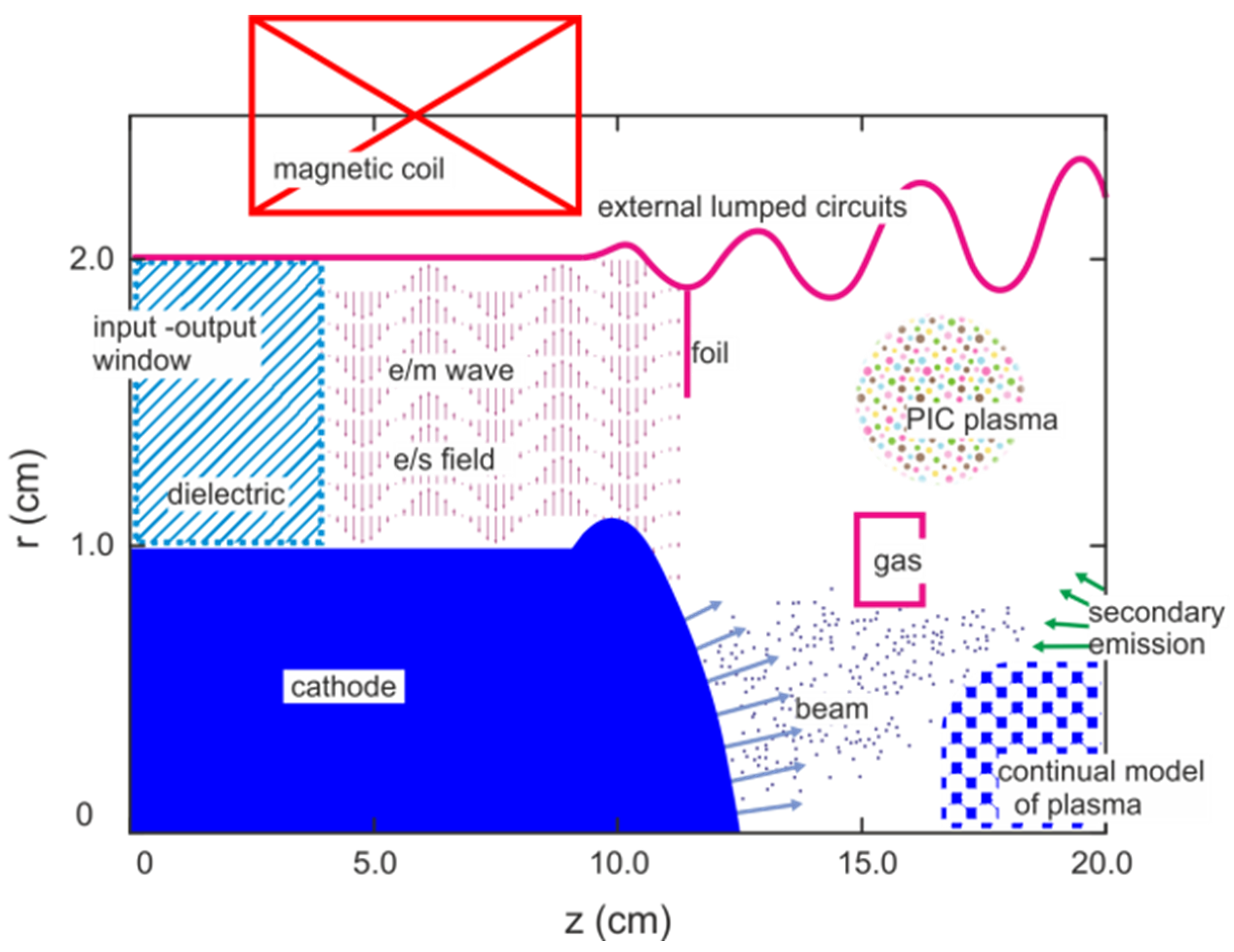
The code KARAT has shown high efficiency in modeling electronic devices such as a reverse wave lamp, vircators, free-electron lasers, beam-plasma discharge, etc., and in modeling the elements of the electromagnetic suppression problem, including a description of the microwave radiation source and the propagation and interaction of radiation with the irradiated object (Figure 1). The code is suitable for modeling devices with electron and ion beams, as well as the laser–plasma interaction. Plasma is modeled by macroparticles and/or hybrid models. If necessary, for example, when describing the penetration of an electron beam into a gas and/or secondary emission from surfaces, a collision simulation can be conducted. The range of problems of non-stationary electrodynamics, in which the code KARAT has long been successfully used and has proven itself well, is illustrated in Figure 1.

There are three components of the code that process one-dimensional, two-dimensional and three-dimensional problems, respectively (hereinafter referred to as 1D, 2D and 3D). In all three cases, all three components of electromagnetic fields and the component of particle pulses are taken into account. The 2D part is modeled in planar (x, z), polar (r, θ) and axisymmetric (r, z) geometries; the 3D part is modeled in Cartesian (x, y, z) and cylindrical (r, θ, z) geometries. The code can perform simulations in electromagnetic or potential approximations.

At the origin of the PiC code KARAT is a three-dimensional self-consistent electrodynamic model, where electric E and magnetic B fields are found from Maxwell’s equations:

$$\nabla \times B=\frac{4\pi }{c}J+\frac{1}{c}\frac{\partial E}{\partial t},$$

(1)

$$\nabla \times E=-\frac{1}{c}\frac{\partial B}{\partial t},$$

(2)

where J is the current density. Fields E and B satisfy different boundary conditions depending on the types of boundaries of the computational domain (including ideally conductive surfaces, surfaces with finite conductivity and open boundaries). The launch of an external electromagnetic pulse is carried out by implementing boundary conditions corresponding to the type of wave. The system (1) to (2) is solved by the finite difference method (FDTD) on a rectangular grid with a shift in space and time.

To solve Maxwell’s equations, a difference scheme with stepping over on rectangular grids with a shift is used. The specific implementation of the circuit used in the code has the property of accurately describing the boundary conditions on the borders of the computational domain. Testing on problems with analytical solutions shows a significant advantage of the scheme used over other options for the accuracy of the law of conservation of energy.

The current density at each point in the computational domain is determined only within the PiC method:

$$J=\frac{1}{∆V}{\displaystyle \sum _s{Q}_s}{v}_s,$$

(3)

where $v_s$ is the velocity of the particle with the index s, $Q_s$ is the part of the charge of the particle in this unit cell and $∆V$ is the volume of the unit cell. Since electrons in a system can have relativistic velocities, the relativistic equation of motion of a charged particle in an electromagnetic field is used to describe the motion of macroparticles.

$$\frac{dp}{dt}=Q\left(E+\frac{1}{c}v\times B\right),$$

(4)

where p and v are the momentum and velocity of the macroparticle, wherein

$$p=m_{p}v\gamma ,\gamma =1/\sqrt{1-\frac{v^2}{c^2}},$$

(5)

where $m_p=\eta m$ is the mass of the macroparticle, $Q=\eta q$ is its charge, m and q are the mass and charge of the real plasma particles (electrons and ions) and η is the enlargement parameter (merging factor). Equations (1)–(5) constitute a complete system that allows a self-consistent description of the dynamics of particles and the electromagnetic fields they generate. For a detailed description of the code KARAT finite difference scheme, see Appendix A.

The external magnetic field is specified in several ways, namely, by describing the magnetic coils and setting the field value on the axis of the system, as well as directly setting the field in the region. The latter option involves the use of information from other specialized codes or the results of real measurements. The quasistatic electric field is given by specifying potentials on the boundary electrodes and then solving the Laplace equation in volume.

Methods for describing the boundaries and elements of the computational domain made it possible to describe all the options encountered in practice—many hundreds of problem statements. In particular, foils under certain potentials, including those with particle absorption, can be included in the computational domain; at the boundaries, conditions for launching electromagnetic waves inside and/or releasing them to the outside can be set (Figure 1). This makes it possible to simulate the connection to the supply coaxial of sources described by lumped parameters in the form of RLC circuits.

The mass and charge of macroparticles can be orders of magnitude higher than the mass and charge of real plasma particles (electrons and ions), and yet, under certain conditions, the results of PiC modeling with a high degree of accuracy coincide with the results of a real experiment and analytical solutions. Indeed, in equation of motion (4), the mass and charge of the particle are included in the form of a relation. The dynamics of macroparticles do not differ from the dynamics of real plasma particles. However, when determining the current density J, the charge of the macroparticle is explicitly included in Formula (3), and the magnitude of the merging factor η can affect the results of the simulation. Note that the main limitations of the PiC modeling of laser-plasma processes on a personal computer are the number of macroparticles used in the calculation and the number of grid nodes, which currently cannot significantly exceed the order of 10⁷.

3. Mathematical Model of the Simulation of Nuclear Reactions in KARAT Code

The uniqueness of the KARAT code also lies in the fact that it is one of the very few where nuclear reactions can be simulated, in particular, the reaction D + D → ³He + n (DD reaction) with the release of neutrons and the aneutronic proton–boron reaction with the release of almost only alpha particles. This section describes in detail, as a simpler case, the algorithm for modeling the DD reaction in laser-driven plasmas, and also discusses some specifics of the more complex simulation of the proton–boron fusion.

The development of petawatt-level lasers in the last decades has led to the implementation of such conditions and modes of exposure to ultra-intense laser radiation on gas, cluster and solid-state targets, in which there is an effective formation of beams of high-energy electrons and ions, the interaction of which with the substance of the target leads to the generation of bremsstrahlung gamma quanta and various nuclear and photonuclear reactions. As a result, the picosecond relativistic laser plasma created is the unique object that allows in the laboratory to simulate and investigate the extreme states of matter related to the problems of controlled thermonuclear fusion. In addition to basic research, such laser-plasma particle sources are of great interest for various applications, such as radiography, hadron therapy, nuclear waste disposal, etc.

For example, laser exposure to targets containing deuterium, high-energy deuterons (deuterium nuclei), can enter in a fusion DD reaction with the release of neutrons. Measuring the parameters of such neutrons is an effective method for studying fast deuterons, especially those that, under the action of a laser pulse on solid-state targets, have been accelerated deep into the target. To obtain quantitative information about the energy spectrum and angular distribution of deuterons according to the study of neutron fluxes, an approach is often used in which the motion of a deuteron in the target volume, taking into account ionization losses and neutron emission, was modeled by the Monte Carlo method.

The mathematical model contains a two-dimensional PiC code, with the help of which the distribution function at velocities of fast deuterons accelerated during the laser action is calculated, and a Monte Carlo code that uses the resulting distribution function as an initial condition for calculating the neutron emission when fast deuterons interact with the resting deuterons of the target is used. At the same time, the model of the Monte Carlo code has laid down the following basic assumptions: the distribution of deuterons is symmetrical with respect to the axis of the laser pulse and the target is “thick” enough that all fast deuterons completely lose their energy to ionize the atoms in the target volume. One of the disadvantages of this model is the impossibility of taking into account the dynamics of heating the target atoms when they interact with beams of electrons and deuterons accelerated by a laser pulse. Note also that such a Monte Carlo code fundamentally does not allow modeling the emission of neutrons during the interaction with counter beams of deuterons, which can occur when the laser irradiation of targets with a complex structure, in particular, hollow or layered targets, takes place.

Meanwhile, in the code KARAT, from the first principles, the probability of a DD reaction at each time step for each deuteron is calculated in the process of self-consistent PiC modeling by the interaction of an ultra-intense laser pulse with a target containing deuterium ions. This method of modeling neutron emissions not only makes it possible to obtain results that correspond well to experimental data on neutron emission during the irradiation of “thick” targets from deuterated polyethylene, but also to investigate the case of layered targets in which the neutron yield increases significantly.

The model of the neutron generation unit integrated into the KARAT code is based on the formula for the cross-section of the DD synthesis reaction in the laboratory reference frame, which, according to known semi-empirical data, is written in the following form:

$${\sigma }_{dd}(E_0)=(107.4+0.33E_0)E_0^{-1}\exp \left(-44.4/\sqrt{E_0}\right),$$

(6)

where $E_0$ is the energy of the fast deuteron in kiloelectronvolts and ${\sigma }_{dd}$ is the cross-section in Barns (=10⁻²⁴ cm²).

In the process of simulating the action of an ultra-intense laser pulse on a target containing deuterons, at each step in time for each primary macroparticle corresponding to the deuteron moving at a speed $\overrightarrow{V}$, the probability of the act of fusion reaction is calculated as follows. Over the entire computational domain, the density of deuterons is $n_d$, their average velocity is ${\overrightarrow{V}}_{av}$ and the root mean square spread of velocities is ${\overrightarrow{V}}_T$ over each Cartesian coordinate in the reference frame moving at speed ${\overrightarrow{V}}_{av}$. The relative velocity ${\overrightarrow{V}}_{rel}$ of the primary deuteron and the random deuteron of the target at that node is then calculated

$${\overrightarrow{V}}_{rel}=\overrightarrow{V}-{\overrightarrow{V}}_{av}-{\overrightarrow{V}}_T\cdot \left(\chi -0.5\right),$$

(7)

where $\chi$ is a random number from the interval from 0 to 1. For the kinetic energy $E_0$ corresponding to this velocity, Formula (6) calculates the total cross-section $\sigma$ of the reaction and finally finds the probability $P$:

$$P=A\cdot \sigma \cdot \left|V_{rel}\right|\cdot n_d\cdot ∆t,$$

(8)

where $∆t$ is the step in time. The presence of the second term in Formula (7) ensures the absence of DD reactions; for example, in the monoenergetic beam of deuterons, when $\overrightarrow{V}={\overrightarrow{V}}_{av}$, at the same time, the presence of the third term in Formula (7) allows us to take into account in Formula (8) the heating of the target deuterons due to laser action. No restrictions are imposed on the velocity values ${\overrightarrow{V}}_{av}$ and ${\overrightarrow{V}}_T$ in Formula (7). Since with the assumed values of the physical parameters of the simulated objects, the probability of reaction is not applied. Since with the assumed values of the physical parameters of the simulated objects, the probability of reaction is expected to be very small, to create conditions for observing the dynamics of neutrons in Formula (8) an artificial coefficient $A$ of increase in the probability of reaction is introduced. When determining the actual neutron yield, the number of neutrons obtained in the calculation is divided by the coefficient $A$.

Further, the probability calculated by the Formula (8) is compared with a random number ξ from the interval from 0 to 1, and if the probability is less than this number, then the transition to the next deuteron is carried out. Otherwise, the act of birth of a neutron with energy of 2.45 MeV begins to play out. First, the deuteron closest to the primary one is found, with a relative kinetic energy close to the energy that was used in calculating the probability. Then, the neutron is launched from the point of the center of mass of the primary and nearest deuterons. In the system of the center of mass, the neutron is launched at a speed of the corresponding energy of 2.45 MeV and at an angle evenly distributed from 0 to 2π radians. After the neutron is launched, its motion is calculated until it arrives at the boundary of the computational domain, where its parameters are fixed. It is believed that the neutron inside the computational domain does not interact with anything. At the neutron launch point, a macroparticle is also launched, simulating the ³He²⁺ ion. Its momentum is calculated on the basis of the conditions for observing the law of conservation of momentum in the described act. It should be noted that similar principles and approaches were also used under the modeling of the DD reaction in a nanosecond vacuum discharge (NVD) [22].

In the case of the aneutronic proton–boron (pB) reaction (p + ¹¹B → α + ⁸Be* → 3α + 8.7 MeV), at each step in time for each proton moving at the velocity $V_p$ in the target area, according to a given cross-section $\sigma (E_p)$ [23], the probability of the reaction act $P=A\sigma (E_p)V_{p}n∆t$ was calculated and compared with a random number ξ ≤ 1. If the probability $P$ turned out to be less than ξ, then the transition to the next proton was carried out; otherwise, a procedure was launched, as a result of which the proton was excluded from the calculation, and alpha particles with energies of 0.9 MeV and 3.9 MeV [24] were launched from its location point. The direction of launch was determined from the law of conservation of momentum.

The ionization energy losses of charged particles during their movement along their trajectory $l$ in a boron target were taken into account according to the well-known Bethe-Bloch formula:

$$\frac{d{E}_{p,\alpha }}{dl}=-\frac{2\pi n{Z}^2{e}^4}{E_{p,\alpha }}\frac{M_{p,\alpha }}{m_e}\ln \frac{4m_e{E}_{p,\alpha }}{M_{p,\alpha }I},$$

(9)

where $E_{p,\alpha }$—the energy of proton or alpha-particle, $M_{p,\alpha }$ and $Z$—their mass and charge, $m_e$ and $e$—the electron mass and charge and $I=13.5 Z_B$ (eV)—the average ionization potential of a boron atom, $Z_B=5$.

Similarly, the yield of the proton–boron reaction was calculated for plasma oscillatory confinement in a nanosecond vacuum discharge. For the early calculations of α-particle yield, a block was used in which the fusion reaction pB was simulated. In addition, a separate block of ⁸Be* decay into two α-particles was also used [25]. The PiC simulation of the proton–boron fusion is discussed in more detail below in Section 5.

4. PiC Simulation of Laser-Driven Proton–Boron Fusion

Let us consider an example of a numerical simulation of the proton–boron reaction, initiated by high-power picosecond laser radiation with a relativistic intensity of 3 × 10¹⁸ W/cm² [20]. The simulation was carried out in a two-dimensional XZ version of the code KARAT and was divided into two stages. At the first stage, the interaction of a laser pulse with a primary aluminum target, on the back surface of which there was a layer of protons, was carried out (Figure 2a). As a result of this interaction, a beam of protons is formed, moving from the back surface of the target. At the second stage, the interaction of the proton beam with a secondary boron target was simulated, accompanied by a pB reaction (Figure 2b).

The computational domain had dimensions of 40 μm along the Z axis and 60 μm along the X axis. The target was a rectangular region of 10 μm along the Z axis and 50 μm wide along the X axis. The target was filled with macroparticles simulating electrons and aluminum ions with a constant concentration n = 10 n_cr = 1.1 × 10²² cm⁻³, where n_cr = 1.1 × 10²¹ cm⁻³. In front of the target was a layer of aluminum preplasma 6 μm thick and 50 μm wide. Preplasma was filled with macro-electrons and aluminum ions. The preplasma concentration profile along the Z axis varied exponentially from a magnitude of 1.1 × 10²⁰ cm⁻³ on the left border to 2.2 × 10²¹ cm⁻³ on the right border. The preplasma concentration profile was homogeneous in the transverse direction of the target. The distance along the Z axis from the left boundary of the computational domain to the left boundary of the preplasma was 4 μm. On the back surface of the target there was a layer 0.2 μm thick and 50 μm wide, consisting of electrons and protons with a concentration of n = 1.1 × 10²² cm⁻³. The distance along the Z axis from the proton layer on the back surface of the target to the right border of the computational domain was 20 μm.

A laser pulse fell on the target from left to right at an angle of 30 degrees to the normal surface of the target. The intensity of the laser pulse was 3 × 10¹⁸ W/cm², with a wavelength λ = 1 μm, a duration τ = 1 ps and a diameter d = 10 μm. The maximum intensity of the laser pulse reached the target at a time of 2 ps. The total duration of the calculation was 5 ps.

The electrons of the preplasma, making complex oscillatory movements in the field of the laser pulse, acquire a component of the velocity in the positive direction of the Z axis. These “hot” electrons pass through the aluminum target and form a quasi-stationary electric field near its back surface, in which the protons on it are accelerated. The amplitude of the electrostatic field can reach a value of the order of 10¹⁰ V/cm, which allows protons to acquire kinetic energy up to 5 MeV.

The integral energy spectrum of the proton beam reaching the right border of the computational domain in the time interval from t = 2.4 ps (the moment when the first protons reach the right boundary) to t = 5 ps is shown in Figure 2b. To calculate the absolute values of protons, we used the assumption that the transverse size of the proton beam along the Y axis (it is not used in the calculation) coincides with the transverse size along the X axis. The number of fast protons with energies above 1 MeV is about 9 × 10¹¹, and the effective temperature of fast protons is 630 ± 30 keV.

At the second stage, the simulation of the pB reaction was performed in the interaction of a proton beam with a boron target (Figure 3a). The energy loss of protons during the movement of the beam through the target is described by Formula (9). The size of the new computational domain was 60 μm along the X axis and 120 μm along the Z axis. To define the proton beam in the nuclear reaction simulation unit, an array of data obtained at the first stage of modeling for protons that reached the right boundary were used. For each proton, the X coordinate, the velocity components (V_x, V_z) and the moment of time of reaching the boundary were recorded. At the second stage, protons with parameters taken from the specified array were launched from the left boundary (Z = 0) of a new computational domain, with a time shift corresponding to the arrival of the first proton on the right boundary in the first stage.

A rectangular boron target with dimensions of 50 μm along the X axis and 100 μm along the Z axis was simulated by an electrically neutral medium with a given concentration of boron atoms n = 2.5 × 10²³ cm⁻³.

As a result of the calculations, the total number of alpha particles N_α = 1.04 × 10⁹ born during the interaction of the proton beam with the boron target was determined, which coincides with the experimental value of the absolute yield of alpha particles [24]. It should be noted that not all alpha particles born during the interaction of a proton beam with a boron target can leave the target and be registered, for example, using CR-39 track detectors. As follows from the calculations, no more than 5% of alpha particles with energy E > 0.5 MeV (which is necessary to be detected using CR-39) leave the target and reach the left boundary of the computational domain, which is in good agreement with the results of the experiment [24].

The energy spectrum of alpha particles that have reached the left boundary of the computational domain is shown in Figure 3b. The spectrum has a local maximum at an energy of E_α = 3.3 MeV, which corresponds to alpha particles with an energy of 3.9 MeV emitted at a depth of about 18 μm from the target surface and lost energy due to ionization losses in accordance with Formula (9). Note that the protons with an energy of 1 MeV on the surface of the target will have an energy of E_p = 0.6 MeV as a result of ionization losses, which is resonant for the cross-section of the proton–boron reaction.

5. PiC Simulation of Proton–Boron Fusion in a Scheme of Plasma Oscillatory Confinement

Essential progress has been obtained in laser-driven pB fusion experiments and the increase in α-particles yield has been observed during the last decade ([26,27,28] and ref. therein). Nevertheless, the proton–boron plasma confinement under extreme conditions in a single device for pB fusion (without any externally applied laser or proton beam irradiation of any boron-containing targets) is of understandable and reasonable interest independently [21]. Remarkably, the inertial electrostatic confinement (IEC) [29] is one of the very few schemes where protons and boron ions can rather easily obtain the energies needed for the observable pB reactions.

An IEC compact scheme with reverse polarity [21,30] based on a miniature nanosecond vacuum discharge (NVD) [31,32,33] turned out to be quite suitable for the implementation and study of processes leading to nuclear reactions. The yields of DD neutrons, both single and pulsating ones, were registered earlier and studied in detail in NVD [22,31,32,33,34], and an aneutronic pB fusion has been demonstrated recently also [21]. The detailed 2D PiC simulations of DD fusion synthesis in NVD [32,33,34] by the code KARAT [2,3] has shown the fundamental role of a virtual cathode (VC) formation and a corresponding deep potential well (PW) [33,34], which accelerates and confines ions.

In short, the processes leading to the synthesis of DD in miniature cylindrical NVD, as shown by PiC modeling in the KARAT code, are as follows. Beams of autoelectrons extracted from the external cathode applied with a high voltage accelerate by radius towards the anode Pd tubes. Further, flying into the anode space through a “grid” of thin Pd tubes, the electron beams slow down as they approach the discharge axis. An excess of electrons in this region forms a very small VC (radius r_vc ≈ 0.1 cm) and a corresponding deep PW (with a depth of φ_pw ≈ 100 kV [21,22]). Simultaneously, the interaction of a part of the autoelectrons with deuterium-loaded Pd anode tubes leads to the formation of an erosive anode plasma near them, containing deuterons and deuterium clusters. Head-on collisions of deuterons accelerated in the PW to the energies of ~100 keV leads to nuclear reactions and to the appearing of DD neutrons. Deuterons are also oscillating in the VC field, and DD synthesis takes place periodically at the PW “bottom” accompanied by the pulsating yield of DD neutrons [31,32]. This scheme of plasma confinement in NVD is called oscillatory confinement (OSCO) [21,22].

A rather similar scenario holds for aneutronic pB fusion in NVD. PiC simulations show that the pB reaction can also be achieved under accelerating and confining protons and boron ions by the field of the VC [25]. The head-on collisions of part of the protons and boron ions with energies of ~100–500 keV in the process of their oscillations in the PW lead to proton–boron fusion. The reaction probabilities were determined using the known experimental and theoretical values of the pB reaction cross-sections embedded in the simulation (Section 3).

For the illustration, the 2D PiC simulations presented below were carried at an applied voltage of U = 100 kV with a voltage front of ∆t_f = 1 ns, which are close to the experimental values used for demonstration of the pB fusion in NVD [21]. Under PiC simulations, there were 300 grid points on the Z axis and 50 on the radius r. The total number of macroparticles was up to 10⁶.

Figure 4a shows the cylindrical geometry of the electrodes with a distance between the anode and the cathode of 0.1 cm. In 2D modeling, a horizontal “plateau” inside the hollow cathode corresponds to very thin Pd anode tubes attached to the end of the Cu anode [34]. On the left, a TEM wave from a high-voltage generator is fed into the coaxial along the Z axis (Figure 4a), which creates an electric field between the anode and the cathode, providing autoelectron emission from the cathode. In this field, the electrons are accelerated along the radius to the center of the discharge (the very small blue dots are shown in Figure 4) and intersect the anode at a distance of r ≈ 0.3 cm (green area, Figure 4a) with an energy of ≈100 keV (Figure 4b). Irradiation of the anode with electron beams leads to the appearance of boron ions and protons in the vicinity of the Pd anode tubes. Penetrating further into the anode space, the electrons are inhibited and reflected by oncoming flows (Figure 4a) and as a result form a VC with a radius of ≈0.1 cm (Figure 4b). There is no external pulsed electric field inside the anode; however, a negative electric charge of the electrons creates a rather deep PW near the axis (Figure 5a). This ensures the acceleration of protons and boron ions further along the radius to the discharge axis Z (r = 0). Here, the velocity and the density of the latter reaches their maximum values (for more details, see [35]).

The potential well with a depth of about 100 kV, which corresponds to the VC of the electrons in the anode space, is shown in Figure 5a (at the 5th ns of the PiC simulation). For the real pB fusion experiment, the anode Pd tubes were filled by hydrogen during electrolysis, and the Pd tube surface with a micro relief developed was also fulfilled by boron nanoparticles [21]. Under the irradiation of Pd anode tubes by energetic autoelectrons, the boron ions and protons will be created near the edge of the PW. In the PiC simulations, the anodic tube (Figure 4a) was also fulfilled by protons and boron ions. The radial acceleration of protons and boron ions in the field of the VC was followed by their oscillations in the deep PW, which simultaneously confines ions during oscillations (see movie from KARAT code in [21]).

The corresponding features of OSCO are illustrated in Figure 5b, where the energies of randomly chosen isolated groups of protons (index r) and boron ions (index y) in the PW during 20 ns of PiC simulations are presented [35]. We see that the PiC simulation recognizes the oscillatory character of the confinement of protons and boron ions in the PW. In fact, the passing of charges through the discharge axis corresponds to their maximum energy; meanwhile, a minimum of kinetic energy corresponds to the full deceleration of ions at the edge of the PW.

Obviously, the oscillation frequencies for protons and boron ions turn out to be rather different (Figure 5b), and this has a bad effect on the pB fusion efficiency [35]. Nevertheless, head-on-like collisions of part of the boron ions and protons with sufficient energies near the discharge Z axis provide a certain number of pB reactions. As an example, the result of the PiC simulation of related secondary α-particles’ yield is presented in Figure 6a. For illustration, the energies of all particles participating in a pB nuclear reaction as a function of their position along the Z axis [25] are shown in Figure 6b (at the same time, when t = 5 ns, the PiC simulated positions of all particles along the discharge radius r can also be found in Figure 4a).

Thus, the modeling by the code KARAT made it possible to clarify the not at all obvious physics of the complex processes leading to pB fusion under plasma oscillatory confinement [21,22]. In particular, the PiC simulations of pB fusion processes have recognized that the plasma of NVD is a quasi-neutral one [35] near the discharge axis. It is rather different from the plasma conditions in the scheme of periodically oscillating plasma spheres (POPSs) developed earlier for fusion in oscillating plasmas [29,36,37]. In addition, unlike the original POPS scheme with thermal plasma, the distribution functions of protons and boron ions are non-Maxwellian in NVD plasma [35]. This means than in our miniature IEC scheme (with reverse polarity [30]) based on NVD, an aneutronic pB synthesis takes place [21] in the periodically appearing nonequilibrium plasmas on the discharge axis which remained “non-ignited” [35].

Earlier in the POPS scheme, a favorable scaling of the growth in the DD fusion power with a decrease in the VC radius was obtained for spherical geometry [36,37]. This means that reducing the size of the new device will make it cheaper, but the release of DD neutrons may increase at the same time. In the cylindrical geometry for NVD, for fusion power we obtained P ~ φ_pw²/r_vc² [35]. It was shown previously that with a decrease in the anode space in the NVD up to the diameter of the anode tube at Ø_A = 0.1 cm that this scaling for DD synthesis can be maintained practically [38]. Of great interest is the question of a similar scaling of the release of an aneutronic pB reaction with a decrease in the VC size. The picture here may be more complicated than for DD fusion, since protons and boron ions differ in mass and charge, and there will be different oscillation frequencies for them in the anode space. In this regard, in continuation of experiments on pB synthesis in NVD with the available geometry of the electrodes (Figure 4a), the novel experiments with a threefold decrease in the diameter of the anode space are planned. In this case, one “translucent” Pd tube with Ø_A = 0.2 cm will be used as the anode, and the diameter of the cylindrical cathode will be Ø_C = 0.4 cm.

In order to have an idea of the expected release of α-particles for new electrode geometry and to determine the optimal discharge parameters, a simulation of the yield of the pB reaction for various combinations of applied voltage and flowing current was carried out in the KARAT code.

Table 1. The yield of α-particles (a.u.) from proton–boron reactions depends on the applied voltage U, kV, and the flowing current I, kA.

U [kV]\I [kA]	1	2	3	4	5
60	0	2.3 × 108	1.6 × 108	1.2 × 108	1.4 × 108
80	0	1.47 × 109	4.5 × 109	3.1 × 109	2.5 × 109
100	0	3.7 × 108	1.9 × 1010	1.8 × 1010	1.6 × 1010
120	0	2.4 × 108	8.2 × 109	3.3 × 1010	3 × 1010
150	0	4 × 106	2.6 × 109	3.6 × 1010	3.8 × 1010

shows the simulated values of the α-particles’ yield in the intervals U = 100–150 kV and I = 1–5 kA (for the voltage front ∆t_f = 3 ns, and during the time t = 10 ns). Indeed, the changing in the α-particles’ release at I = const with an increase in voltage or at U = const with an increase in current are by no means obvious and require further analysis. Nevertheless, taking into account the real experimental possibilities, from the data in Table 1 it can be concluded that the optimal options in the experiment will probably be the values I ≈ 3 kA and U ≈ 100 kV and/or I ≈ 4 kA and U ≈ 120 kV. Comparing the data obtained by modeling the values of the yield of α-particles (Table 1) with their more noticeable release (Figure 6a) for Ø_A = 0.6 cm, it can be preliminarily concluded that the favorable scaling of P ~ φ_pw²/r_vc² with a decrease in the diameter of the anode from Ø_A = 0.6 cm (Figure 4a) to Ø_A = 0.2 cm is very far from being fulfilled. This essential “hint” from the simulation in the KARAT code will be very useful in preparing a real experiment, but the final answer about scaling of the pB fusion power with a decrease in VC size will still have to be given by the experiment itself.

6. Concluding Remarks

The main scope of the electromagnetic code KARAT is a computational experiment in applied problems of engineering electrodynamics. The PiC method for the kinetic description of plasma is implemented in the code. Over the past three decades, numerous problems of non-stationary engineering electrophysics and electrodynamics have been solved with the help of the code KARAT (see [2,3,39,40,41,42,43,44,45,46,47,48,49,50,51] and references therein). In the present work, the results of a numerical simulation within the framework of the code KARAT of the key physical processes leading to the aneutronic proton–boron fusion were presented in detail and discussed both for laser-driven plasma and for plasma under oscillatory confinement. As was shown above by the simulations of pB fusion, a unique feature of the code KARAT is the possibility of a self-consistent modeling of nuclear reactions at each time step in the process of electrodynamic calculation. Using these examples of simulations of pB nuclear synthesis under such different conditions as laser-driven plasma or oscillating plasma confinement in a vacuum discharge, the possibilities of the code KARAT were demonstrated to adequately describe the very complex physical processes leading to aneutronic pB nuclear reactions under extreme conditions in very different experiments where the yields of α-particles were observed.

In fact, the simulation in the code KARAT provides not only an explanation but also formulates new experiments in applied and fundamental non-stationary electrodynamics and predicts possible results in advance. This allows, in principle, the undertaking of new exploratory research with significantly lower costs, including time. In the process of implementing real experiments, simulation in the KARAT code can accompany the experiment, and, if necessary, adjust the directions of experimental activity. For example, under the study of pB fusion in NVD, the code allows us to compare the release of α-particles for different anode–cathode configurations and choose the optimal ones for given Volt-Ampere characteristics of discharge, or to study the effect of the front of applied voltage on the release of α-particles at a given geometry of electrodes [35]. For laser-driven pB plasma, the code KARAT allows us not only to optimize the intensity and duration of laser exposure to the target, but also to take into account additional pB reaction channels as well as the interaction of nuclear reaction products with target atoms [52].

The self-consistent modeling of processes of various physical nature in the code KARAT (laser-driven plasma/microwave photonics + plasma electrodynamics + nuclear reactions) made it possible to obtain results very close to experimental data even under conditions of problems with complex geometry. Note that, in a sense, a somewhat similar self-consistent approach was used in [53], which considers a completely different problem related to the numerical simulation of the interaction between the associated flow occurring near a monoblock moving in a gaseous medium and the combustion products of solid fuel flowing from a solid-fuel rocket engine. The peculiarity of the approach used is the description of gas-dynamic processes inside the combustion chamber, in the nozzle block and in the down jet based on a single calculation methodology.

To date, the presented simulations of pB fusion describe rather well the significant part of the experimental data obtained [20,21,23,35,52]. The synergy of step-by-step numerical modeling and the further development of real experiments will allow us to continue to search for optimal ways to increase the efficiency of aneutronic pB synthesis and increase the yield of α-particles, which are extremely necessary for practice.