1. Introduction
The energy resource of wind power generation is green and environmentally friendly, and the reliability of wind turbines has become a hot research topic in recent years. Pérez et al. [
1] focused on the failure rate of the wind turbine components and found that the gearbox and blades were the most likely locations to cause faults, and they proposed that state detection can improve the reliability of wind turbines. Kusiak and Li [
2] predicted the fault situation of the wind turbine based on data from state detection to ensure its reliability. Chen et al. [
3] proposed a transfer condition monitoring based on feature alignment and parameter fine-tuning for more accurate monitoring, which can more accurately identify the status of wind turbines. Dui et al. [
4] proposed a resilience optimization model of a multi-component system to determine the degree of influence of components on the reliability of the wind turbine system, thus improving the reliability of the wind turbine system. Su et al. [
5] established a stochastic differential equation state model to describe the degradation of wind turbines, preventing wind turbine failure. Research has shown that focusing on the faults and reliability of wind turbine components is necessary to increase the reliability of wind turbines.
Wind turbine gears are one of the core components of the wind turbine system, which transfer power and adjust the wind speed and output torque. If the gear fails, it will directly affect the operating efficiency and output power of the wind turbine, causing the production line to stagnate and resulting in significant losses [
6]. Therefore, the reliability of the gear directly affects the reliability of the wind turbine system. The reliability evaluation of wind turbine gears can predict the probability of gear failure and possible failure modes. It provides necessary information for preventive maintenance of the wind turbine, ensures safe and stable operation of the wind turbine, and can reduce shutdown costs. Reliability-based design optimization methods and control methods to improve the reliability of wind power systems have also been widely recognized and studied in recent years [
7,
8,
9,
10]. In conclusion, the calculation and analysis of gear reliability are very important.
In order to evaluate the reliability of gears more accurately, it is necessary to fully and realistically consider influencing factors such as gear load cycling and material quality. Wind turbine gears subjected to random load changes will experience fatigue damage, resulting in reduced fatigue strength. The decrease in gear strength will cause the problem of tooth surface wear or fatigue fracture during operation, which will affect the reliability of the gears [
11]. The ability of a gear to resist external loads after a certain degree of fatigue damage is defined as the residual strength.
Researchers have proposed a variety of residual strength models. For instance, Schaff and Davidson [
12] proposed a general residual strength model of materials, and its key parameters need to be fitted by the experimental data of materials. Based on the hypothesis of Hahn and Kim [
13], Chou and Croman [
14] established the residual strength model of time by the relationship between strength and life. Ganesan and Joanna [
15] considered the effect of the stress ratio of the continuous load on the component and proposed a two-parameter residual strength model of glass-fiber-reinforced polymer. Cheng and Hwu [
16] obtained the residual strength degradation trajectory of the composite material based on Schaff’s model.
Some researchers have also developed residual strength models for metals, in addition to the residual strength model for composite materials. For instance, in the aspect of damage development, Li et al. [
17] established the residual strength degradation model of the material based on a large number of experimental data of 35CrMo. Gao and An [
18] developed a residual strength model that requires a small amount of data and takes into account the dispersion of residual strength based on the stress interference theory. Based on the fatigue damage theory and the interval theory, Jiang et al. [
19] established a two-parameter residual strength model using experimental data and obtained fuzzy dynamic reliability. In recent years, many researchers have used data-driven methods to predict the degradation of residual strength. For instance, Yang et al. [
20] used an artificial neural network to predict the residual strength of composites after impact. Lu et al. [
21] used principal component analysis combined with a multi-objective optimization vector machine to predict the residual strength of the pipeline. Miao and Zhao [
22] proposed a method of deep extreme machine learning to predict the residual strength of defective pipes. Meng et al. [
23] proposed an adaptive Kriging model to improve the efficiency of optimal design for offshore wind turbines.
In summary, most of the residual strength models are used to describe composite materials. Significantly, there is no consistent residual strength model for both composite materials and metal materials. Furthermore, most of the existing residual strength models require a large amount of experimental data to predict. However, many materials or parts require long experimental cycles and high costs. For this, a simple model based on the fatigue damage accumulation theory is proposed, which requires a small number of parameters. The effect of the loading condition, loading sequence, and interaction between loads on strength degradation is fully considered. Moreover, the degradation trajectory of fatigue strength can only be predicted by understanding the fatigue life data of materials or mechanical parts.
Wind energy is an unstable energy source, with variable wind speeds and directions. Variations in wind speed will impact the load on the gear directly. Furthermore, changes in the operational status of the wind turbine will also affect the gear load. From this point of view, the load on the wind turbine gear shows obvious randomness. Actually, the wind load is not completely irregular. The wind speed in different regions varies seasonally, such as in southeastern China, where the wind speed is usually higher during the winter and summer but weaker in autumn [
24]. In addition, the wind loads vary in different seasons due to the seasonal nature of the loads applied to the gears of wind turbines. As mentioned above, in order to more closely characterize the residual strength of wind turbine gears and more accurately predict their reliability, the stochastic and seasonal nature of the loads to which they are subjected needs to be fully taken into account.
The remainder of the paper is organized as follows. In
Section 2, the boundary conditions of the residual strength model are described, and the existing nonlinear fatigue damage accumulation model is introduced. Based on this model, a residual strength model considering the loading sequence and load interaction is established. The experimental data of two materials are used to validate the proposed residual strength model and compare it with Schaff’s model. In
Section 3, the main fatigue failure modes of the wind turbine gear are analyzed, and the fatigue life curve of the gear is obtained by modeling and simulation. Then, the statistical analysis of the four-season wind load on the gear is carried out, and the degradation trend of the residual strength of the gear is obtained. In
Section 4, the reliability of wind turbine gear is obtained by the Monte Carlo simulation method based on the random stress-residual strength interference theory.
Section 5 summarizes some main conclusions and proposes some further study directions.
2. Residual Strength Model of Multistage Loading Based on the Fatigue Damage Accumulation Theory
The strength degradation of materials has always been a hot topic in the field of reliability. The gear will suffer fatigue damage under the continuous action of cyclic loads. From a macro perspective, the fatigue damage of materials can be evaluated by measuring the residual strength changes of the material [
25]. Thus, it can be considered that the strength degradation is closely related to the degree of fatigue damage accumulation. Conversely, the trend of residual strength degradation can also be measured by fatigue damage. Based on these theories, the existing nonlinear fatigue cumulative damage theories are introduced. We then explain the boundary conditions of the residual strength model. Finally, a residual strength model for multistage loading is proposed from the perspective of cumulative fatigue damage, and the proposed model is validated.
2.1. Nonlinear Fatigue Damage Accumulation Model
To date, the linear damage accumulation theory proposed by Miner is widely used in engineering, since its form is concise and simple for calculation [
26]. With the development of damage theory, it is found that damage is not only related to the size of the load but also to the loading sequence and the interaction between the loads. Due to the fact that fatigue damage of gears is a complex nonlinear process in practical engineering, establishing a nonlinear damage model is more practical. Many researchers have established nonlinear damage accumulation models from different perspectives. Manson and Halford [
27] used the damage curve method to establish a nonlinear damage accumulation model. Freudenthal and Heller [
28] developed a fatigue damage model considering the interaction between variable amplitude loads. Zhu and Huang [
29] established a damage model based on the law of creep. Zhu et al. [
30] introduced the energy damage parameter to define uncertain fatigue damage. Risitano et al. [
31] quantified fatigue damage accumulation based on the relationship between temperature and loads.
Considering the loading sequence effect, Peng et al. [
32] proposed a nonlinear damage accumulation model based on the energy method, which can be formulated as
where
is fatigue damage,
is the number of load cycles, and
is the fatigue life of parts or materials.
The model is verified by 45 steel, 16 Mn steel, and Al-2024 aluminum alloy. It is found that the damage prediction has good accuracy.
By integrating Equation (1), the following expression can be obtained:
From the above equation, it can be seen that when
, the cumulative damage
. When
, the total cumulative damage
reaches 1. If the load is applied once more, the material will fail. Therefore, the material fails when the number of load cycles is
[
26,
33].
2.2. Boundary Conditions of the Residual Strength Model
In general, the residual strength of the material is related to the initial strength of the material, the quality of processing and manufacturing, the loading method of the load, and the size of the load. According to the existing residual strength model [
34,
35], it can be found that the formula generally satisfies the following two conditions:
(1) The initial residual strength is the static strength of the material.
where
is the residual strength of the load 0 times and
is the static strength.
(2) When the material or part fails, the residual strength is equal to the peak value of the load.
where
is the maximum value of the load on the part or material.
Among numerous residual strength models, the model proposed by Schaff is quite consistent with various practical situations. Due to the fewer parameters required to determine and its relatively high accuracy, this model is widely used in practical engineering applications. Schaff’s model contains two parameters: The initial residual strength and the maximum value of the load, which also meet the boundary conditions of Equations (3) and (4) mentioned above. Therefore, a residual strength model based on Schaff’s model [
12] is proposed, which can be formulated as
where
should make the residual strength expression satisfy the above two boundary conditions, which can be formulated as
The decrease in residual strength is related to the degree of fatigue damage accumulation. It is also found that
satisfies the condition of
. Thus, let
. We substitute Equation (2) into Equation (5) to obtain the residual strength model considering the loading sequence effect, which can be formulated as
From Equation (7), it can be seen that the proposed residual strength model satisfies the initial state of static strength, and the load on the material at failure is equal to the maximum load. With the increase in loading times , the residual strength decreases monotonously. Using this model, the residual strength degradation law of the material under the load can be obtained.
2.3. Residual Strength Model under Multistage Loading
In engineering practice, mechanical components are usually subjected to constantly changing loads. Therefore, it is necessary to consider how to characterize residual strength when loading multistage loads. If the residual strength model of the two-level load is known, then the residual strength model of the multistage load only needs to be analogized on this basis. Therefore, in this paper, we derive the residual strength model expression of two levels for load.
If the first-level loads and the second-level loads are applied separately to the same material, the rate of decline of the two residual strengths will necessarily be different. In other words, there are two different curves. According to the equivalent theory of fatigue damage accumulation, it is necessary to equalize the residual strength of the first-level loads to the residual strength curve of the second-level loads. Therefore, a suitable equivalence formula needs to be established to perform the equivalence of the residual strength under different levels of loading. The equal percentage reduction in residual strength under different loads is defined as the equivalent basis. The percentage expression of the decrease in residual strength can be formulated as
The percentage of residual strength reduction after the first-level loads is equal to the percentage of residual strength reduction after the second-level loads, which can be formulated as
In the theory of fatigue damage accumulation, some researchers considered the interaction between loads [
33,
36]. The ratio of the two-level load is introduced into the expression of damage equivalence to characterize this influencing factor. In this paper, this theory is also applied to the residual strength equivalent theory, and the load ratio factor is introduced into the equivalent expression. Then, the equivalent residual strength can be formulated as
where
is the number of first-level actions to load,
is the number of times that the residual strength after the first level of loads is equivalent to the second level of loads, and the second level of loads need to be applied.
is the mean stress of the first level of loads and
is the mean stress of the second level of loads.
Based on the concept of fatigue damage theory, the residual strength of two levels of load is equivalent. The equivalent loading number
of the second-level load can be obtained and added to the original loading number
of the second-level load to obtain the remaining strength after the second-level load is loaded. Therefore, it is necessary to derive the equivalent loading number
of the second-level load. Substituting the residual strength formula (7) into formula (11) can obtain
By simplifying Equation (12), the equivalent number of actions
can be obtained, which can be formulated as
The first level of loads are
times, and the residual strength after
times of the second level of loads are equivalent to
times of the second level of loads. The residual strength after two levels of loads can be obtained, which can be formulated as
In summary, when the material is subjected to the multistage load, the calculation is performed according to the above ideas based on the residual strength equivalent theory.
2.4. Verification of Residual Strength Model
At present, the typical residual strength model is Schaff’s model. Due to its few parameters and high precision, it is widely used in practical engineering. The degradation model described by Schaff’s model is generally consistent with the actual degradation situation. Therefore, the proposed model is compared with the typical Schaff’s model in this section. The materials used to verify model performance include the residual strength data of 45 steel under first-level loading and the experimental data of 30CrMnSiA steel under second-level loading from the published literature [
32].
2.4.1. One-Level Loading
45 steel was subjected to a constant amplitude load of 310.37 MPa. The number of load cycles, the experimental residual strength data, the residual strength predicted by Schaff’s model, and the residual strength predicted by the proposed model are shown in
Table 1.
The calculation results of the two models are compared, as shown in
Figure 1.
In
Table 1, it can be seen that the calculation results of Schaff’s model are closer to the second and third points of the experiment. However, the overall results of the proposed model perform better predictive performance. In
Figure 1, it can be seen that the maximum error of Schaff’s model is 7.45% and the maximum error of the proposed model is 5.07%, indicating that the error of the proposed model is closer to the true value. The
of Schaff’s model is 0.9870, while the
of the proposed model is 0.9901, indicating that the predicted residual strength of the proposed model fits better with the actual value. Both Schaff’s model and the proposed model show a decreasing pattern of strength in their residual strength curves. The residual strength decays slowly in the early stages and decreases abruptly in the later stages, leading to sudden failure of the material.
2.4.2. Two-Level Loading
The experimental data of 30CrMnSiA and aluminum alloy Al-2024 is also used to validate the proposed model [
32]. Both materials are subjected to two levels of horizontal loading, and the experimental data of the two materials in different load sequences are shown in
Table 2 and
Table 3.
Schaff’s model and the proposed model are used to calculate the residual strength degradation curve of the material under two levels of sequential loading, as shown in
Figure 2 and
Figure 3.
In order to evaluate the predictive performance of the model, the maximum error and the goodness of fit between the predicted and true values are calculated, as shown in
Figure 4 and
Figure 5.
From
Figure 4 and
Figure 5, it can be clearly seen that the
of the proposed model is higher than that of Schaff’s model for both materials, regardless of the high-to-low loading order or the low-to-high loading order. The maximum error of the proposed model is smaller than that of Schaff’s model. Therefore, it can be considered that the proposed residual strength model has high accuracy for both high-to-low loading and low-to-high loading. Moreover, in
Figure 2 and
Figure 3, it can be seen that the loading sequence has an impact on the strength degradation trend of the load. Therefore, it is necessary to consider the loading sequence of the load in predicting the trend of strength degradation. The proposed model reflects this influencing factor well, which indicates that it is suitable for residual strength prediction.
4. Analysis of the Residual Strength and Dynamic Reliability of Gear
In general, the strength degradation of machine parts and materials is closely related to the properties of the materials and the loads to which they are subjected. The load on the wind turbine gear is random. The uncertainty of the load makes the strength degradation uncertain. The randomness of strength degradation makes the reliability analysis and prediction of mechanical structures more complex and difficult. Therefore, in order to better predict wind turbine gear bending failure, it is necessary to fully consider the randomness of strength degradation. In this section, the residual strength variation trend and dynamic reliability of gear under multistage random loads in spring, summer, autumn, and winter are calculated and analyzed.
4.1. Residual Strength Model for Tooth Root Bending Strength
If the equivalent stress of a season is considered a one-level load, then the gear will be subjected to four-level loads every year, in the order of spring, summer, autumn, and winter. After each level of load is applied, Equation (14) needs to be used for residual strength equivalence, and then the residual strength after the next level of load is calculated. The corresponding life after
times of bending stress is also the random variable that follows a certain distribution, so the residual strength has randomness at the determined time
. Next, we calculate the residual strength of the gear according to Equations (7) and (14) for residual strength. However, it is difficult to calculate the residual strength of the gear under such a multistage random load using conventional probability methods. Therefore, the Monte Carlo method is used to deal with such problems because of its good adaptability and randomness. It can be applied to address various problems and can simulate the relationship between a variety of complex probability distributions and random variables [
49,
50]. As the number of simulations increases, the simulation results are closer to the real situation and can provide more accurate estimates [
51]. The flowchart for calculating the residual strength of gear using the Monte Carlo method is shown in
Figure 15.
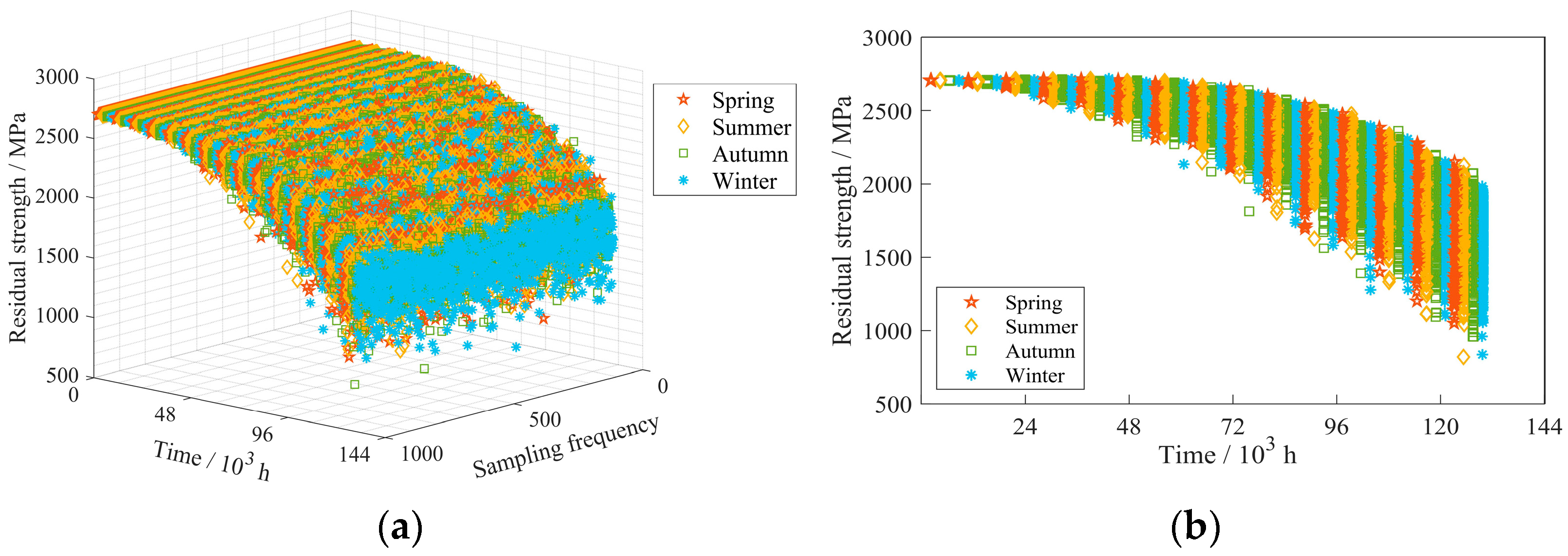
We calculate the residual strength at the end of each season and obtain the residual strength path of the gear within 15 years. The calculation results are shown in
Figure 16.
In
Figure 16, it can be seen that the residual strength of the gear shows the degradation trend over time. Due to the randomness of stress, the residual strength of the gear also represents randomness. At time
, the residual strength of the gear is not a fixed value but a random variable that follows a distribution. As the service life increases, the range of gear residual strengths gradually widens. In order to better describe the law of the residual strength of gear, the distribution of the residual strength is fitted for each season. In general, a two-parameter Weibull distribution can be used to describe the residual strength distribution after any given fatigue cycle [
16]. The Q-Q and CDF tests show that the residual intensity at the end of each season follows a Weibull distribution. Taking the spring residual strength of the first year as an example, the shape parameter of the fitted Weibull distribution is 34,678.07, and its scale parameter is 3746.73. The test results of the Q-Q chart are shown in
Figure 17.
The fitted Weibull distribution is close to the actual residual strength quantile and the Q-Q plot is in a straight line, and between each quantile and the diagonal is 0.9938. From the non-parametric CDF test, it can be seen that the maximum vertical difference between the actual data and the fitted data is very small, and the two CDF curves almost coincide. Therefore, it can be considered that using the Weibull distribution to fit the residual strength at time is reasonable.
Since the residual strength of time
can be described by the Weibull distribution, the distribution of residual strength changing with time can be described by the Weibull distribution of parameters changing with time. After obtaining the scale and shape parameters of the Weibull distribution fitted by residual strength at the end of each season, the variation of the parameters over time is analyzed. The fitting results of parameters over time are shown in
Figure 18.
The coefficient of determination of scale parameters is 0.9855 and the coefficient of determination of the shape parameter is 0.9986. Both values are very close to 1, indicating that the fitting result is relatively suitable. Therefore, the residual strength of gears follows a two-parameter Weibull distribution, and the scale parameter
and shape parameter
at time
can be formulated as
4.2. Gear Reliability Analysis Considering the Failure of Tooth Root Bending
There are many methods for reliability analysis. For instance, Huang et al. [
52] combined the chi-square approximation and numerical integration methodologies to calculate the reliability of positioning accuracy. Li et al. [
53] used a Bayesian copula network based on a fuzzy rough set to evaluate and make decisions. Yazdi et al. [
54] used an improved fault tree method to analyze reliability. Yan et al. [
55] evaluated the reliability of multiple failure modes based on the method of failure modes and effects criticality analysis. The performance of mechanical components usually varies over time and there are multiple failure modes. Yu et al. [
56,
57,
58,
59] have studied the time-varying reliability calculation method for complex products. In this section, in addition to calculating the static reliability of gears for four seasons, the time-varying reliability of gears is also considered.
The stress level of gear varies in different seasons, and it can be assumed that the stress distribution of the four seasons does not change with the increase in gear operating years. In other words, within the prediction of 15 years, it can be assumed that the stress level remains constant throughout the four seasons of each year. Without taking into account the degradation in the strength of the gear, the stress–strength interference theory suggests that the reliability of the gear in the same season will remain the same regardless of the year. According to the calculation, the reliability of gears at the end of spring, summer, autumn, and winter is 0.9995, 0.9988, 0.9973, and 0.9964, respectively. It can be seen that the reliability of gear is the highest in spring.
When considering the strength degradation of a gear, the stress on the gear is a seasonal distribution, and the remaining strength of the gear is a temporal distribution. Based on the stress strength interference theory, the criterion for gear failure is that if the residual strength is less than the random load, the gear will fail. The reliability and failure rate results are calculated by the Monte Carlo method, as shown in
Figure 19 and
Figure 20.
In
Figure 19 and
Figure 20, it can be seen that the reliability of gear does not monotonically decrease over time but rather has a significant span from the end of winter to the end of spring each year. Although the decreasing trend of residual strength is continuous, the load on the gear varies from season to season as a result of the influence of stress levels. The explanation diagram of the reliability jump is shown in
Figure 21.
The remaining strength of the gear gradually decreases over time. The strength of the gear at the end of spring in the first year is , and after one year of service, the strength of the gear at the end of winter in the second year is . The stress level of gear in spring is lower than the stress level in winter. The stress level is only related to the season and does not change with the increase in service life. The strength at the end of spring in the first year is higher than the strength at the end of winter in the first year. Under the influence of stress and strength, the reliability of spring in the first year is higher than that of winter. The residual strength at the end of spring in the second year is lower than the strength in winter in the first year, but the stress level in spring is much lower than the stress level in winter. The reliability at the end of spring in the second year will be higher than that at the end of winter in the first year.
As mentioned above, it can be concluded that the differences in stress levels among different seasons have a significant impact on gear reliability. The reliability trend over the four seasons is determined by both the stress level and residual strength of the gear concurrently. In the spring of each year, the reliability of the gear is the highest, since the load on the gear is the smallest, and the residual strength of the gear is the highest. This result is consistent with the reliability results of the gear without considering strength degradation. The changes in stress levels throughout the four seasons do not make the reliability of gear monotonically decrease over time, but rather experience a sudden increase in reliability.
By observing the variation pattern of reliability at the same stress level, the following three aspects can be determined:
The overall decreasing trend of reliability is determined by the degradation trend of gear strength. The gear’s reliability in each season decreases monotonically from year to year, which indicates that the reliability of the gear has decreased compared to the previous year in all seasons. Due to the sudden increase in the decay rate of the residual strength, the reliability of the gear suddenly decreases rapidly in the 15th year.
By observing the distance between the four seasonal reliability curves, it can be found that the distance between the summer and autumn reliability curves is the largest, the distance between the spring and summer curves ranks second, and the distance between the autumn and winter curves is the smallest. It can be considered that the impact of load amplitudes in the four seasons causes a change in the distance between the reliability curves of adjacent seasons. In
Table 4, it can be seen that there is a significant difference in load amplitudes between summer and autumn, resulting in a significant downward shift in the reliability curve from summer to autumn. The difference in amplitude between autumn and winter loads is the smallest, so the overall downward movement of the reliability curve from autumn to winter is relatively small.
The difference in reliability between the four seasons is relatively small in the first few years. In the first nine years, the reliability of gears fluctuated between 1 and 0.99 per year. As the service life increases, the reliability difference of the gear in the four seasons of the same year becomes increasingly significant. In the 15th year, the reliability fluctuation range of the gear within one year is 0.99 to 0.94. This is affected by the randomness of decreasing residual gear strength. As time passes, the range of residual gear strength increases, resulting in a greater range of changes in gear reliability throughout the year.


