Abstract
The development of artificial intelligence systems assumes that a machine can independently generate an algorithm of actions or a control system to solve the tasks. To do this, the machine must have a formal description of the problem and possess computational methods for solving it. This article deals with the problem of optimal control, which is the main task in the development of control systems, insofar as all systems being developed must be optimal from the point of view of a certain criterion. However, there are certain difficulties in implementing the resulting optimal control modes. This paper considers an extended formulation of the optimal control problem, which implies the creation of such systems that would have the necessary properties for its practical implementation. To solve it, an adaptive synthesized optimal control approach based on the use of numerical methods of machine learning is proposed. Such control moves the control object, optimally changing the position of the stable equilibrium point in the presence of some initial position uncertainty. As a result, from all possible synthesized controls, one is chosen that is less sensitive to changes in the initial state. As an example, the optimal control problem of a quadcopter with complex phase constraints is considered. To solve this problem, according to the proposed approach, the control synthesis problem is firstly solved to obtain a stable equilibrium point in the state space using a machine learning method of symbolic regression. After that, optimal positions of the stable equilibrium point are searched using a particle swarm optimization algorithm using the source functional from the initial optimal control problem statement. It is shown that such an approach allows for generating the control system automatically by computer, basing this on the formal statement of the problem and then directly implementing it onboard as far as the stabilization system has already been introduced.
Keywords:
stabilization; optimization; symbolic regression; synthesized control; evolutionary computations; quadcopter model; ordinary differential equations MSC:
49M99
1. Introduction
Long ago, Leonard Euler spoke about the optimal arrangement of everything in the world: “For since the fabric of the universe is most perfect and the work of a most wise Creator, nothing at all takes place in the universe in which some rule of maximum or minimum does not appear”. Striving for optimality is natural in every sphere.
In order to optimally move an autonomous robot to a certain target position, currently, as a standard, engineers first solve the problem of optimal control, obtain the optimal trajectory, and then solve the additional problem of moving the robot along the obtained optimal trajectory. In most cases, the following approach is used to move the robot along a path. Initially, the object is made stable relative to a certain point in the state space. Then, the stability points are positioned along the desired path and the object is moved along the trajectory by following these points from one point to another [1,2,3,4,5,6,7]. The difference between the existing methods is in solving the control synthesis problem to ensure stability relatively to some equilibrium point in the state space and in the location of these stability points.
Often, to ensure stability, the model of the control object is linearized relative to a certain point in the state space. Then, for the linear model of the object, a linear feedback control is found to arrange the eigenvalues of the closed-loop control system matrix on the left side of the complex plane. Sometimes, to improve the quality of stabilization, control channels or components of the control vector are defined that affect the movement of an object along a specific coordinate system axis of the state space. Then controllers, as a rule PI controllers, are inserted into these channels with the coefficients that are adjusted according to the specified control quality criterion [3,4]. In some cases, analytical or semi-analytical methods are used to solve the control synthesis problem and build nonlinear stable control systems [5,7]. But the stability property of the nonlinear model of the control object, obtained from the linearization of this model, is generally preserved only in the vicinity of a stable equilibrium point.
The main drawback of the approach when the control object is moved along the stable points on the trajectory is that even if this trajectory is obtained as a solution of the optimal control problem [8], then the movement itself will never be optimal. To ensure optimality, it is necessary to move along the trajectory at a certain speed, but when approaching the stable equilibrium point, the speed of the control object tends to zero.
The optimal control problem generally does not require ensuring the stability of the control object. The construction of a stabilization system that provides the stability of the object relative to some equilibrium point in the state space is carried out by the researcher to achieve predictable behavior of the control object in the vicinity of a given trajectory.
The optimal control problem in the classical formulation is solved for a control object without any stabilization system; therefore, the resulting optimal control and the optimal trajectory will not be optimal for this object with a further introduced stabilization system. It follows that the classical formulation of the optimal control problem [9] is missing something as far as its solution cannot be directly implemented in the real object, since this leads to an open-loop control. The open-loop control system is very sensitive to small disturbances, but they are always possible in real conditions, since no model accurately describes the control object. In order to achieve optimal control in a real object, it is necessary to build a feedback control system, which should provide some additional properties, for example stability relative to the trajectory or points on this trajectory. The authors of [10] proposed an extended formulation statement of the optimal control problem, which has additional requirements established for the optimal trajectory. The optimal trajectory must have a non-empty neighborhood with a property of attraction. Performing these requirements provides implementation of the solution of the optimal control problem directly in the real control object.
In [11,12], an approach to solving the extended optimal control problem on the base of the synthesized control is presented. This approach ensures obtaining a solution of the optimal control problem in the class of practically implemented control functions. According to this approach, initially, the control synthesis problem is solved. So, the control object becomes stable in the state space relatively to some equilibrium point. In the second stage, the optimal control problem is solved by determination of optimal positions of the stable equilibrium point. Switching stable points after a constant time interval ensures moving the control object from initial state to the terminal one optimally according to the given quality criterion. Optimal positions of stable equilibrium points can be far from the optimal trajectory in the state space; therefore, a control object does not slow down its motion speed. Studies of synthesized control in various optimal control problems have shown that such control is not sensitive to perturbations and can be directly implemented in a real object [13,14].
In synthesized control, the optimal control problem is solved for a control object already with a stabilization system. Another advantage of synthesized control is that the position of the stable point does not change during the time interval; that is, an optimal control function is solved using the class of piece-wise constant functions, which simplifies the search for the optimal solution.
It is possible that piece-wise constant control in the synthesized approach finds several optimal solutions with practically the same value of the quality criterion. This circumstance prompted in us the idea to find among all almost-optimal solutions one that is less sensitive to perturbations. This approach is called adaptive synthesized control.
In this work, a principle of adaptive synthesized control is proposed in Section 2, methods for solving it are discussed in Section 3 and further in the Section 4, a computational experiment to determine the solution of the optimal control problem for the spatial motion of quadcopter by adaptive synthesized control is considered.
2. Adaptive Synthesized Control
Consider the principle of adaptive synthesized control for solving the optimal control problem in its extended formulation [10].
Initially, the control synthesis problem is solved to provide stability of the control object relatively some point in the state space. In the problem, the mathematical model of the control object in the form of ordinary differential equation system is given.
where is a state vector, , is a control vector, , is a compact set that determines restrictions on the control vector.
The domain of admissible initial states is given
To solve the problem numerically, the initial domain (2) is taken in the form of the finite number of points in the state space:
Sometimes, it is convenient to set one initial state and deviations from it:
where is a given initial state, is a deviations vector, , ⊙ is Hadamard product of vectors, is a binary code of the number j. In this case .
The stabilization point as a terminal state is given by
It is necessary to find a control function in the form
where , such that it minimizes the quality criterion
where is the time of achieving the terminal state (5) from the initial state , is determined by an equation
is a particular solution from initial state , , of the differential Equation (1) with an inserted control function (6)
is a given accuracy for hitting to terminal state (5), is a given maximal time for control process, p is a weight coefficient.
Further, using the principles of synthesized optimal control the following optimal control problem is considered. The model of control object in the form (9) is used
where the terminal state vector (5) is changed into the new unknown vector , which will be a control vector in the considered optimal control problem.
In accordance with the classical formulation of the optimal control problem, the initial state of the object (10) is given
In the engineering practice, there can be some deviations in the initial position; therefore, in adaptive synthesized control, instead of one initial state (11) the set of initial states used are defined by Equation (4). The vector of initial deviations is defined as a level of disturbances.
The goal of control is defined by achievement of the terminal state
The quality criterion is given
where is a terminal time, is not given but is limited, , is a given limit time of control process.
According to the principle of synthesized control, it is necessary to choose time interval and to search for optimal constant values of the control vector for each interval
where M is a number of intervals
So the system (10) with the found optimal constant values of the control vector (14) in the right-hand side of differential equations has a particular solution which reaches the terminal state (12) from the given initial state (11) with an optimal value of the quality criterion (13).
Algorithmically, in the second stage of the adaptive synthesized control approach, the optimal values of the vector are found as a result of the optimization task with the following quality criterion, which takes into account the given grid according to the initial conditions:
where K is number of initial states, is determined by Equation (8).
3. Methods of Solving
As described in the previous section, the approach based on the principle of adaptive synthesized optimal control consists of two stages.
To implement the first stage of the approach under consideration for solving the control synthesis problem (1)–(9), any known method can be used. For linear systems, for example, methods of modal control [15] can be applied, as well as such analytical methods such as backstepping [16,17] or synthesis based on the application of the Lyapunov function [18]. In practice, stability is ensured through linearization of the model (1) in the terminal state and setting PI or PID controllers in control channels [19,20]. All known analytical and technical methods have their limitations, which mostly depend on the type of the model used to describe the control object. The mathematical formulation of the stabilization problem as a control synthesis problem is needed to apply numerical methods and automatically obtain a feedback control function. Today, to solve the synthesis problem for nonlinear dynamic objects of varying complexity, modern numerical methods of machine learning can be applied [21]. Among different machine learning techniques, only symbolic regression allows searching both for the structure of the needed mathematical function and its parameters. In our case, the needed function is a control function. So, in the present paper machine learning by symbolic regression [22,23] is used.
Methods of symbolic regression search for the mathematical expression of the desired function in the encoded form. These methods differ in the form of this code. The search for solutions is performed in the space of codes by a special genetic algorithm.
Let us demonstrate the main features of symbolic regression on the example of the network operator method (NOP), which was used in this work in the computational experiment. To code a mathematical expression NOP uses an alphabet of elementary functions:
- –
- Functions without arguments or parameters and variables of the mathematical expression
- –
- Functions with one argument
- –
- Functions with two arguments
Any elementary function is coded by two digits: the first one is the number of arguments, the second one is the function number in the corresponding set. These digits are written as indexes of elements in the introduced sets of the alphabet (17)–(19). The set of functions with one argument must include the identity function . Functions with two arguments should be commutative, associative and have a unit element.
NOP encodes a mathematical expression in the form of an oriented graph. Source-nodes of the NOP-graph are connected with functions without arguments, while other nodes are connected with functions with two arguments. Arcs of the NOP-graph are connected with functions with one argument. If on the NOP-graph some node has one input arc, then the second argument is a unit element for the function with two arguments connected with this node.
Let us define the following alphabet of elementary functions:
With this alphabet the following mathematical expressions can be encoded in the form of NOP:
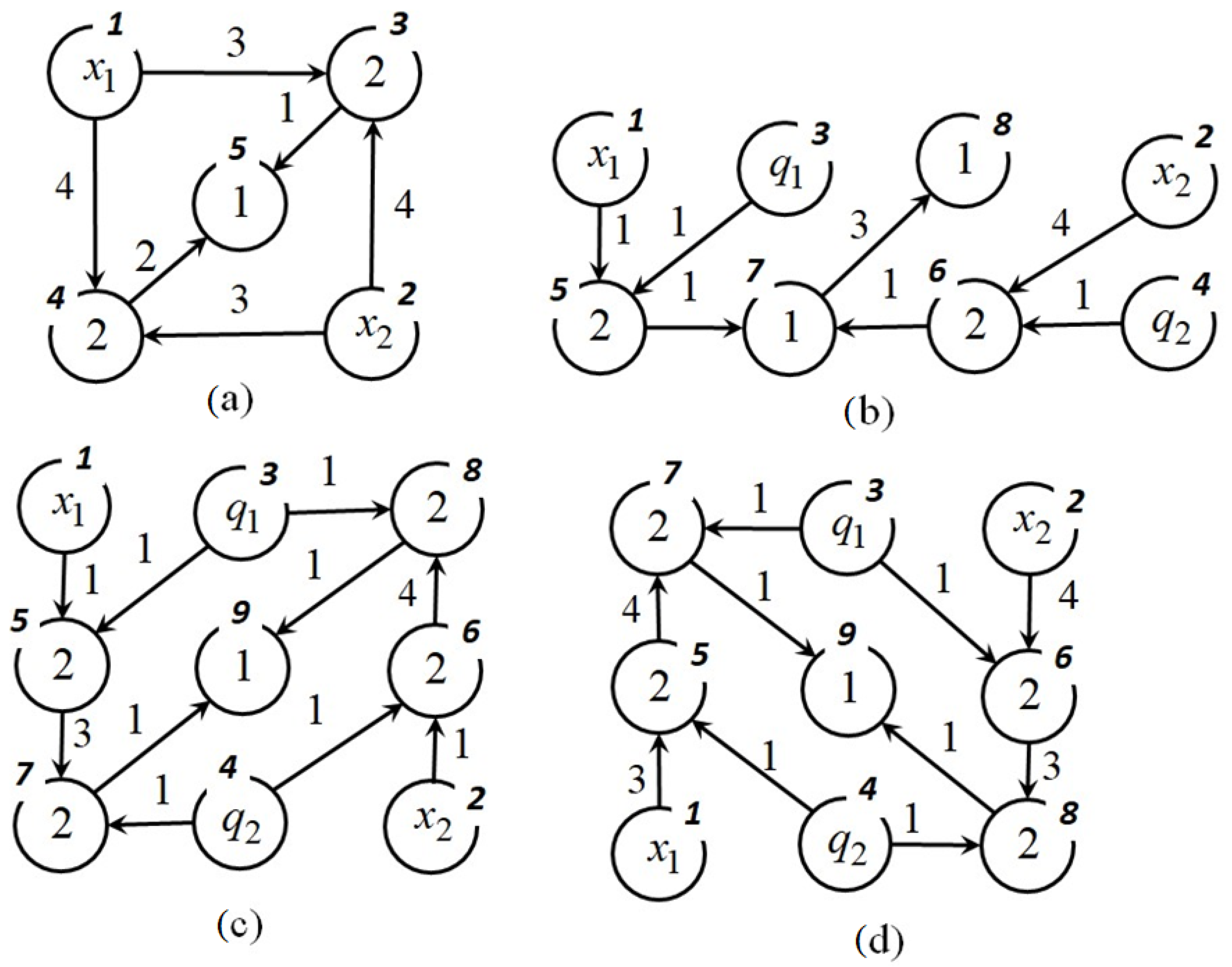
The NOP-graphs of these mathematical expressions are presented in Figure 1. The nodes of the graph are numbered. Inside each node there is either the number of a binary operation or an element of the set of variables and parameters , and the arcs of the graph indicate the numbers of unary operations.
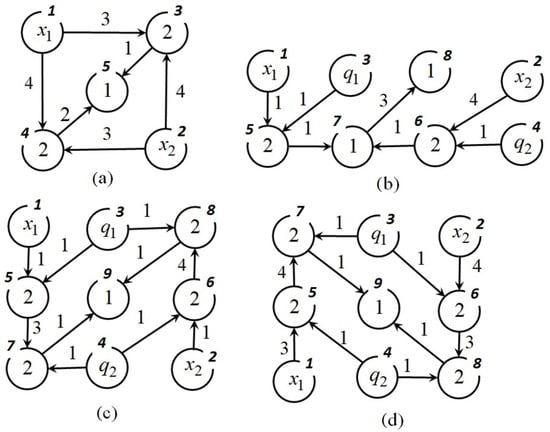
Figure 1.
NOP-graphs for mathematical expressions (21), (a) , (b) , (c) , (d) .
In the computer memory, the NOP-graphs are presented in the form of integer matrices.
As the NOP-nodes are enumerated in such a way that the node number from which an arc comes out is less than the node number to which an arc enters, then the NOP-matrix has an upper triangular form. Every line of the matrix corresponds some node of the graph. Lines with zeros in the main diagonal corresponds to source-nodes of the graph. Other elements in the main diagonal are the function numbers with two arguments. Non-zero elements above the main diagonal are the function numbers with one argument.
To calculate a mathematical expression by its NOP-matrix, initially, the vector of nodes is determined. The number of components of the vector of nodes equals to the number of nodes in a graph. The initial vector of nodes includes variables and parameters in positions that correspond to source nodes, as well as other components equal to the unit elements of the corresponding functions with two arguments. Further, every line of the matrix is checked. If element of the matrix does not equal zero, then corresponding element of the vector of nodes is changed. To calculate mathematical expression by the NOP-matrix, the following equation is used:
where
is a unit element for function with two arguments ,
Consider an example of calculating the second mathematical expression in (21) on its NOP-matrix .
The initial vector of nodes is
Further, all strings in the matrix are checked and non-zero elements are found.
The last mathematical expression coincides with the needed mathematical expression for (21).
So, we considered the way of coding in the NOP method. Then, to search for an optimal mathematical expression in some task, the NOP method applies a principle of small variations of a basic solution. According to this principle, one possible solution is encoded in the form of the NOP-matrix . This solution is the basic solution and it is set by a researcher as a good solution. Other possible solutions are presented in the form of sets of small-variation vectors. A small variation vector consists of four integer numbers
where is a type of small variation, is a line number of the NOP-matrix, is a column number of NOP-matrix, is a new value of an NOP-matrix element. There are four types of small variations: is an exchange of the function with one argument, if , then ; is an exchange of the function with two arguments, if , then ; is an insertion of the additional function with one argument, if , then ; is an elimination of the function with one argument, if and , , and , , then .
The initial population includes H possible solutions. Each possible solution except the basic solution is encoded in the form of the set of small variation vectors
where d is a depth of variations, which is set as a parameter of the algorithm.
The NOP-matrix of a possible solution is determined after application of all small variations to the basic solution
Here, the small variation vector is written as a mathematical operator changing matrix .
During the search process sometimes the basic solution is replaced by the current best possible solution. This process is called a change of an epoch.
Consider an example of applying small variations to the NOP-matrix . Let and there are three following small variation vectors:
After application of these small variation vectors to the NOP-matrix , the following NOP-matrix is obtained:
This NOP-matrix corresponds to the following mathematical expression:
Similar to a search engine, a genetic algorithm is used. To perform the main genetic operation of crossover, two possible solutions are selected randomly
A crossover point is selected randomly . Two new possible solutions are obtained as the result of exchanging elements of the selected possible solutions after the crossover point:
The second stage of the synthesized principle under consideration is to solve the problem of optimal control via determination of the optimal position of the equilibrium points. Studies have shown that for a complex optimal control problem with phase constraints, evolutionary algorithms allow the system to cope with such problems. Good results were demonstrated [24] by such algorithms as a genetic algorithm (GA) [25], a particle swarm optimization (PSO) algorithm [26,27,28], a grey wolf optimizer (GWO) algorithm [29] or a hybrid algorithm [24] involving one population of possible solutions and all three evolutionary transformations of GA, PSO and GWO selected randomly.
4. Computational Experiment
Consider the optimal control problem for the spatial motion of a quadcopter. In the problem, the quadcopter should move for a minimum time on a closed-loop circle from the given initial state to the same terminal state, avoiding collisions with obstacles and passing through the given areas.
4.1. Mathematical Model of Spatial Movement of Quadcopter
In the general case, the mathematical model of a quadcopter as a hard body has the following form:
where F is a summary thrust force of all drone screws, m is a mass of drone, g is acceleration of gravity, , , , are control moments around the respective axes.
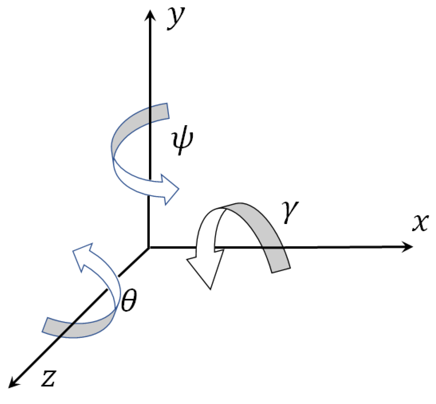
Figure 2 shows how the angles of a quadcopter turn are linked with its axes.
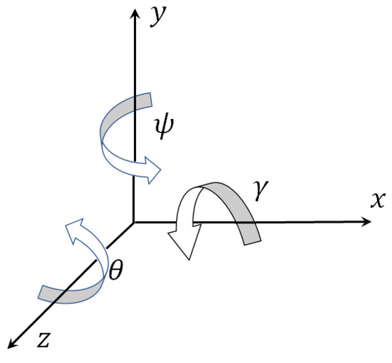
Figure 2.
Inertial coordinate system for quadcopter.
To transform the model (32) to a vector record, the following designations are entered: , , , , , , , , , , , , , , .
As a result the following mathematical model is received:
where is a state space vector, , is a vector of control moments, .
As a rule, quadcopters are manufactured with some angle stabilization systems. This means that a drone can be stabilized at any angle for some interval. The system of angle stabilization provides a stable location of the drone relatively, given angles by control moments:
Assume that the angular stabilization system works out the given angles of the quadcopter quickly enough, at least in comparison with spatial movement. In this case we can assume that the control of the spatial movement of the quadcopter is carried out using the angular position of the drone and the thrust force. Let us define components of the spatial control vector: , , , .
As a result we receive the following model of spatial quadcopter movement:
In this work, this model is used to obtain optimal control for the spatial motion of the quadcopter.
4.2. The Optimal Control Problem for Spatial Motion of Quadcopter
The model (35) of the control object is given. Here, is a state space vector, , is a control vector . is a compact set that defines restrictions on values of control vector components,
According to the principle of synthesized control, initially the control synthesized problem (1)–(9) is solved. The model (35) is used as a model of the control object. To construct the set of initial states (4), the following vector of deviations is used:
In the problem, initial state and terminal state were equal:
For calculation of the quality criterion (7), the following parameters are used: , , .
To solve the control synthesis problem, the network operator method [23] was used. NOP found the following solution:
where
, , , , , .
In the second stage, the optimal control problem is considered. In the problem, the mathematical model (35) is given. The initial state coincides with the terminal state (38).
It is necessary to find a control in the form of points in the state space (14). For synthesized control it is necessary to minimize the following quality criterion:
where , , ,
, , , , , , , , , ,
, , , , , ,+ , , , , , , , , , .
In the optimal control problem, the terminal time is determined by the Equation (8) with , . It is necessary to find coordinates of control points on each time interval, . The desired vector includes parameters, where
that is, . The hybrid evolutionary algorithm has found the following optimal solution:
For the found solution (48), the value of the quality criterion is .
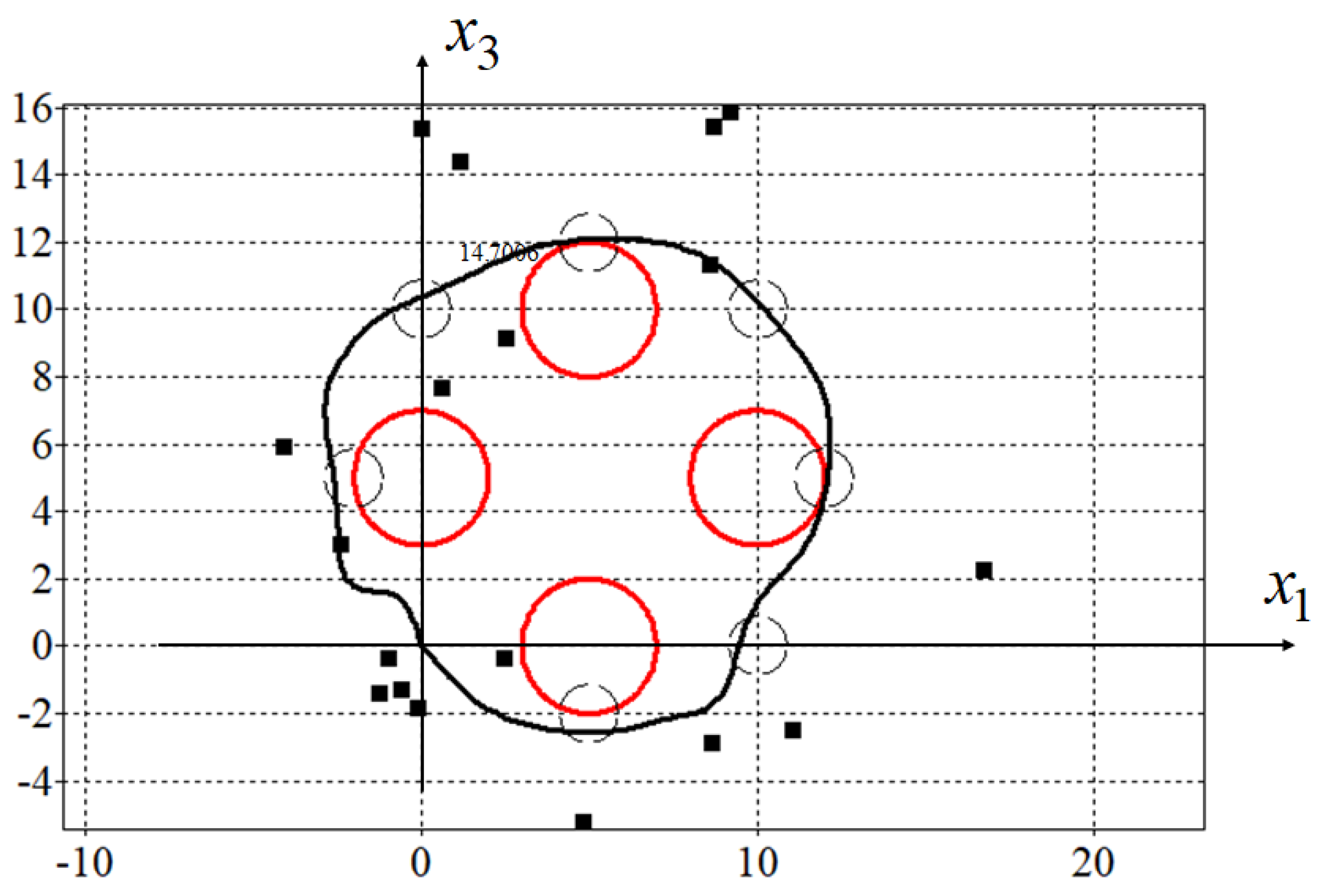
In Figure 3, projections of the optimal trajectory on the horizontal plane are presented. Here, red circles are phase constraints described by (45), small black circles are passing areas described by (46) and small black boxes are control points (48).
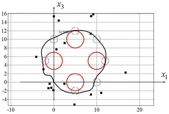
Figure 3.
Optimal trajectory for synthesized control.
For the new adaptive synthesized control proposed in this paper, the set of initial states is determined by Equation (3) with deviation vector
It is necessary to find the same number of control points according to the following quality criterion:
where , is defined by Equation (8). Other parameters of the criterion are the same as for the criterion (44).
Again, the hybrid algorithm was applied and the following optimal solution has been found:
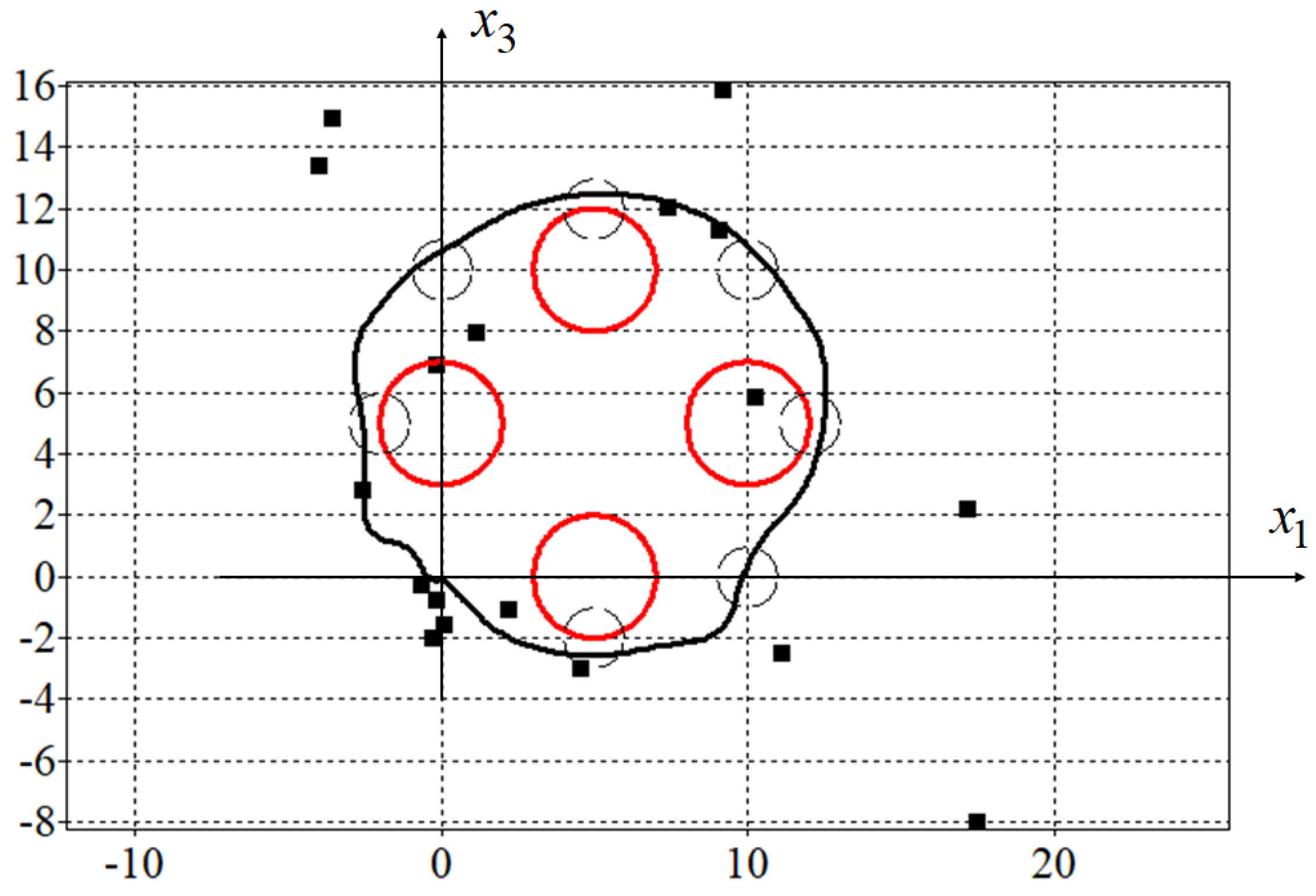
A value of the quality criterion (50) for one initial state , is . In Figure 4, projections of the optimal trajectory on the horizontal plane found by the adaptive synthesized control (51) are presented.
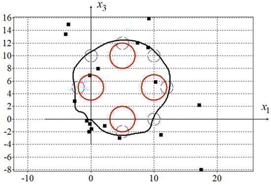
Figure 4.
Optimal trajectory for adaptive synthesized control.
Since the initial state in the problem coincided with the terminal state, in order to force the control object to move along a closed path, mandatory conditions for passing through certain areas were added to the quality criterion. For trajectories that meet the criteria for passing through the specified areas, the value of the quality criterion will not change at . This is seen in Figure 3 and Figure 4 as both trajectories pass through all specified areas.
Let us check the sensitivity of the obtained solutions to random perturbations of the initial state
where is a function generator of random noise, which returns a random number from interval at every call, is a constant level of noise.
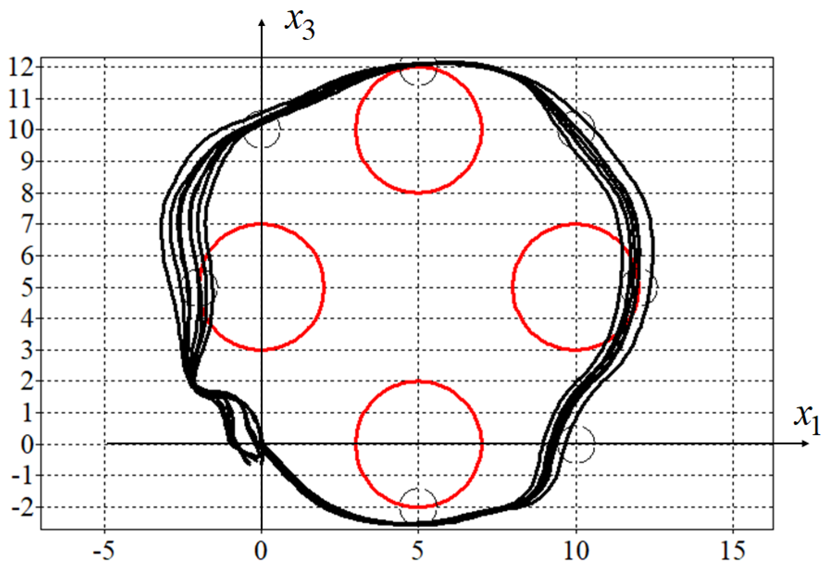
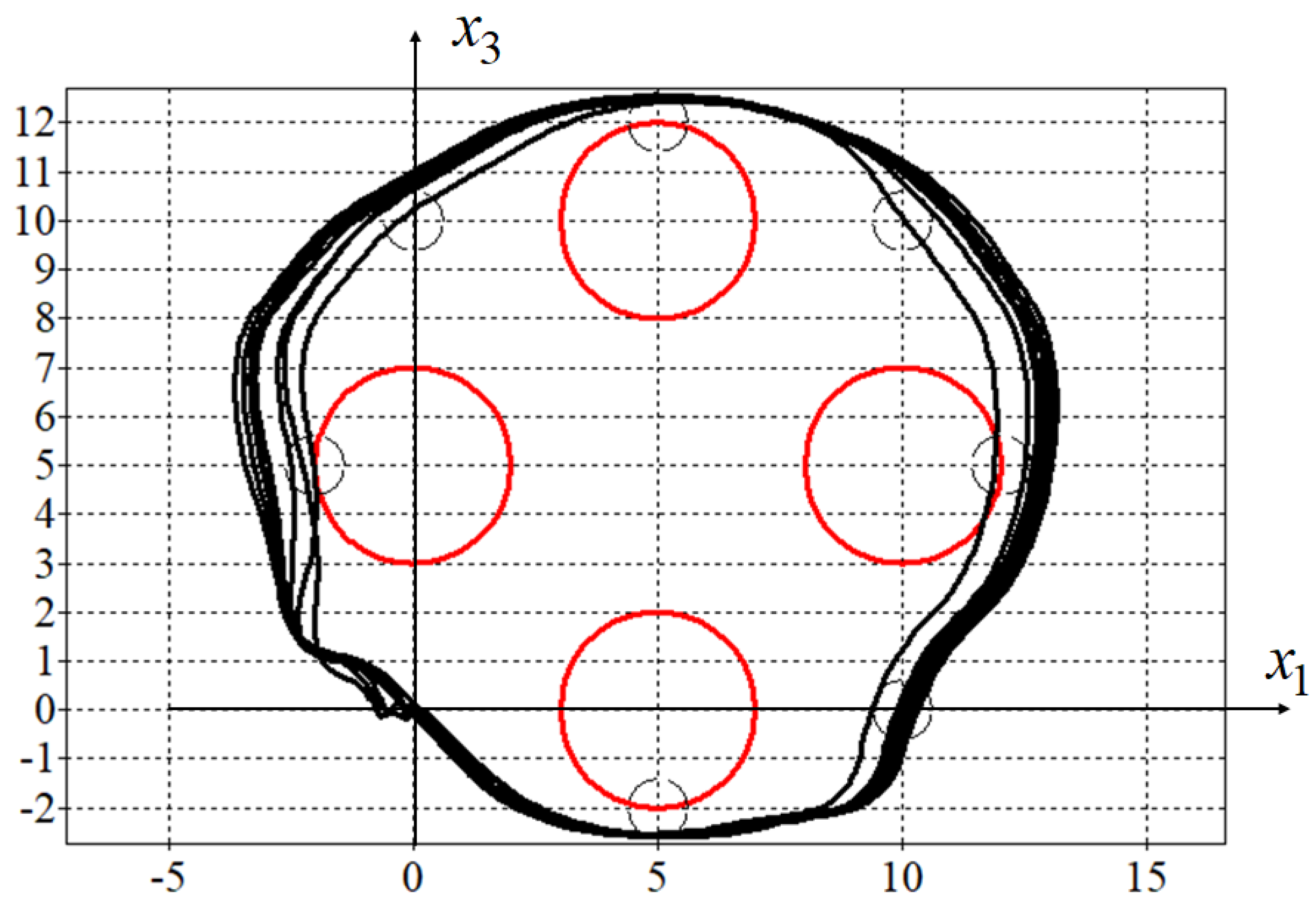
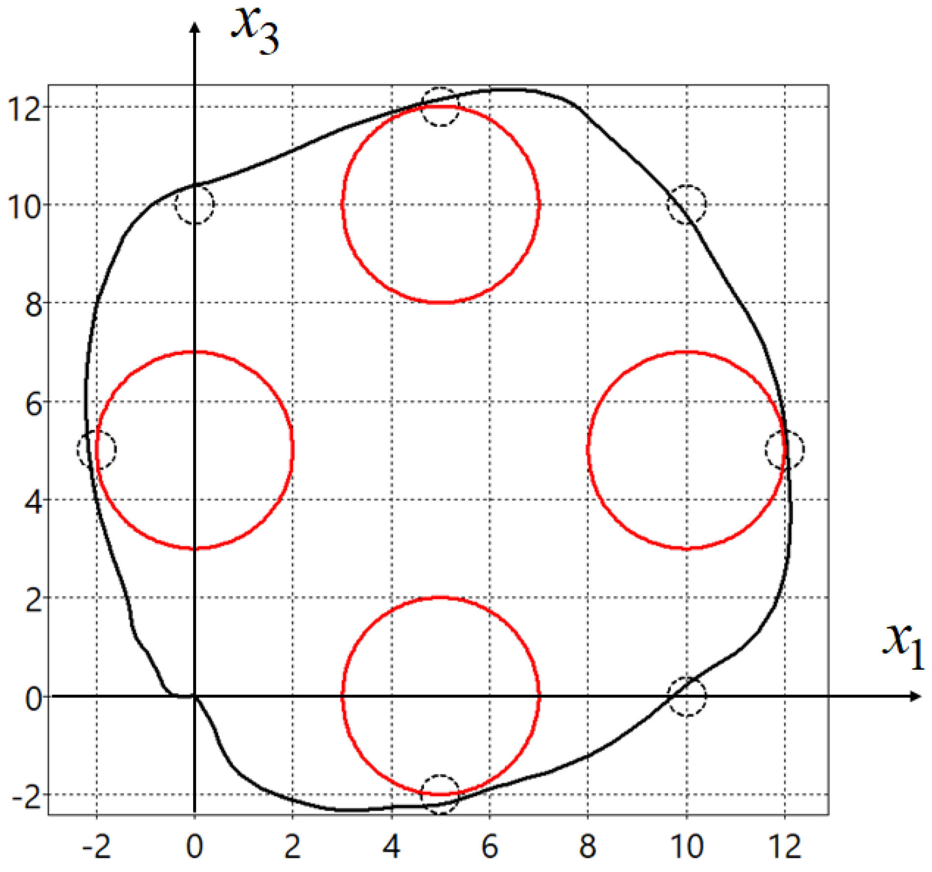
In Figure 5 and Figure 6, the optimal (in blue) and eight perturbed trajectories (in black) for for the solutions obtained by synthesized (Figure 5) and adaptive synthesized (Figure 6) control are presented.
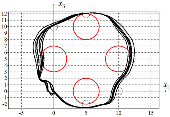
Figure 5.
Optimal and eight disturbance trajectories of synthesized control.
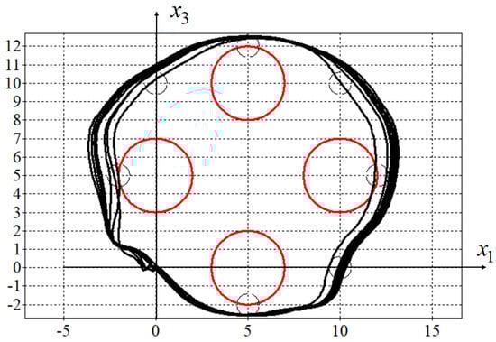
Figure 6.
Optimal and eight disturbance trajectories of adaptive synthesized control.
For comparison, for a model (35) without stabilization systems (39), the problem of optimal control directly was solved, where control was sought in the form of a piece-wise linear function, taking into account restrictions (36).
where
, , is a component of desired parameters vector, ,
In this work, we set the same time interval ; therefore, from (15) , and it is necessary to find parameters,
To solve the optimal control problem, the same hybrid algorithm was used. As a result, the following solution was obtained:
In Figure 7, the projection of the optimal trajectory obtained by the direct method is presented.
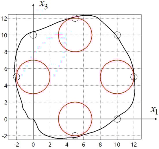
Figure 7.
Optimal trajectory of direct control.
In Table 1 there are values of the quality criterion (44) of ten experiments for perturbed solutions obtained by the synthesized (column Synthesized), the adaptive synthesized (column Adaptive) control and the direct solution (Direct). In two last strings of the table, average values of the functionals and standard deviations for all experiments are presented.

Table 1.
Sensitivity of decisions to perturbations of initial states.
5. Conclusions
A new method for solving the problem of optimal control in the class of implemented functions, an adaptive synthesized control principle is presented. Unlike synthesized control, the new method takes into account the perturbations of the initial state when solving the optimal control problem. Therefore, the value of the quality criterion is calculated as the sum of the quality criterion values for the different initial states. As a result of this approach, a solution is chosen in such a way that for the origin initial state it may not give the best quality criterion value, but in the case of disturbances of the initial state, the quality criterion value changes slightly.
6. Discussion
Obtaining a solution based on replacing the optimal solution is less optimal, but also less sensitive to disturbances. At first glance, this seems obvious and can be applied to any method of solving the optimal control problem. However, this is not the case. A direct solution to the optimal control problem results in control in the form of a time function and an open-loop control system. Perturbation of the initial conditions for such a system gives large variations in quality criterion values, which cannot be reliably estimated from the average value due to the large variance.
The synthesized control method firstly makes the control object stable relative to some equilibrium point in the state space. This means that the perturbed and unperturbed trajectories at each point in time move towards a stable equilibrium point. The adaptive synthesized control method sets the positions of the equilibrium points so that all disturbed trajectories are located in some tube that does not violate phase constraints whenever possible.
In the future, when using the adaptive synthesized control method, it is necessary to assess the required size of the initial state region and reduce the number of initial state points, since this significantly increases the time for finding the optimal solution.
Author Contributions
Conceptualization, E.S.; methodology, A.D. and E.S.; software, A.D. and E.S.; validation, E.S.; formal analysis, A.D.; investigation, E.S.; writing—original draft preparation, A.D. and E.S.; writing—review and editing, E.S. All authors have read and agreed to the published version of the manuscript.
Funding
This research was supported by the Ministry of Science and Higher Education of the Russian Federation, project No. 075-15-2020-799.
Institutional Review Board Statement
Not applicable.
Informed Consent Statement
Not applicable.
Data Availability Statement
Not applicable.
Conflicts of Interest
The authors declare no conflict of interest.
References
- Egerstedt, M. Motion Planning and Control of Mobile Robots. Ph.D. Thesis, Royal Institute of Technology, Stockholm, Sweden, 2000. [Google Scholar]
- Walsh, G.; Tilbury, D.; Sastry, S.; Murray, R.; Laumond, J.P. Stabilization of trajectories for systems with nonholonomic constraints. IEEE Trans. Autom. Control 1994, 39, 216–222. [Google Scholar] [CrossRef]
- Samir, A.; Hammad, A.; Hafez, A.; Mansour, H. Quadcopter Trajectory Tracking Control using State-Feedback Control with Integral Action. Int. J. Comput. Appl. 2017, 168, 1–7. [Google Scholar] [CrossRef]
- Allagui, N.Y.; Abid, D.B.; Derbel, N. Autonomous navigation of mobile robot with combined fractional order PI and fuzzy logic controllers. In Proceedings of the 2019 16th International Multi-Conference on Systems, Signals & Devices (SSD), Istanbul, Turkey, 21–24 March 2019; pp. 78–83. [Google Scholar] [CrossRef]
- Chen, B.; Cao, Y.; Feng, Y. Research on Trajectory Tracking Control of Non-holonomic Wheeled Robot Using Backstepping Adaptive PI Controller. In Proceedings of the 2022 7th Asia-Pacific Conference on Intelligent Robot Systems (ACIRS), Tianjin, China, 1–3 July 2022; pp. 7–12. [Google Scholar] [CrossRef]
- Karnani, C.; Raza, S.; Asif, A.; Ilyas, M. Adaptive Control Algorithm for Trajectory Tracking of Underactuated Unmanned Surface Vehicle (UUSV). J. Robot. 2023, 2023, 4820479. [Google Scholar] [CrossRef]
- Nguyen, A.T.; Nguyen, X.-M.; Hong, S.-K. Quadcopter Adaptive Trajectory Tracking Control: A New Approach via Backstepping Technique. Appl. Sci. 2019, 9, 3873. [Google Scholar] [CrossRef]
- Lee, E.B.; Marcus, L. Foundations of Optimal Control Theory; Robert & Krieger Publishing Company: Malabar, Florida, 1967; 576p. [Google Scholar]
- Pontryagin, L.S.; Boltyanskii, V.G.; Gamkrelidze, R.V.; Mishchenko, E.F. The Mathematical Theory of Optimal Process. L. S. Pontryagin, Selected Works; Gordon and Breach Science Publishers: New York, NY, USA; London, UK; Paris, France; Montreux, Switzerland; Tokyo, Japan, 1985; Volume 4, 360p. [Google Scholar]
- Shmalko, E.; Diveev, A. Extended Statement of the Optimal Control Problem and Machine Learning Approach to Its Solution. Math. Probl. Eng. 2022, 2022, 1932520. [Google Scholar] [CrossRef]
- Diveev, A.; Shmalko, E.Y.; Serebrenny, V.V.; Zentay, P. Fundamentals of synthesized optimal control. Mathematics 2020, 9, 21. [Google Scholar] [CrossRef]
- Shmalko, E.Y. Feasibility of Synthesized Optimal Control Approach on Model of Robotic System with Uncertainties. In Electromechanics and Robotics; Smart Innovation, Systems and Technologies; Ronzhin, A., Shishlakov, V., Eds.; Springer: Singapore, 2022; Volume 232. [Google Scholar]
- Shmalko, E. Computational Approach to Optimal Control in Applied Robotics. In Frontiers in Robotics and Electromechanics. Smart Innovation, Systems and Technologies; Ronzhin, A., Pshikhopov, V., Eds.; Springer: Singapore, 2023; Volume 329. [Google Scholar]
- Diveev, A.; Shmalko, E.Y. Stability of the Optimal Control Problem Solution. In Proceedings of the 8th International Conference on Control, Decision and Information Technologies, CoDIT, Istanbul, Turkey, 17–20 May 2022; pp. 33–38. [Google Scholar]
- Simon, J.D.; Mitter, S.K. A theory of modal control. Inf. Control 1968, 13, 316–353. [Google Scholar] [CrossRef]
- Jouffroy, J.; Lottin, J. Integrator backstepping using contraction theory: A brief methodological note. In Proceedings of the 15th IFAC World Congress, Barcelona, Spain, 21–26 July 2002. [Google Scholar]
- Zhou, H.; Liu, Z. Vehicle Yaw Stability-Control System Design Based on Sliding Mode and Backstepping Contol Approach. IEEE Trans. Veh. Technol. 2010, 59, 3674–3678. [Google Scholar] [CrossRef]
- Febsya, M.R.; Ardhi, R.; Widyotriatmo, A.; Nazaruddin, Y.Y. Design Control of Forward Motion of an Autonomous Truck-Trailer using Lyapunov Stability Approach. In Proceedings of the 2019 6th International Conference on Instrumentation, Control, and Automation (ICA), Bandung, Indonesia, 31 July–2 August 2019; pp. 65–70. [Google Scholar] [CrossRef]
- Zihao, S.; Bin, W.; Ting, Z. Trajectory Tracking Control of a Spherical Robot Based on Adaptive PID Algorithm. In Proceedings of the 2019 Chinese Control And Decision Conference (CCDC), Nanchang, China, 3–5 June 2019; pp. 5171–5175. [Google Scholar] [CrossRef]
- Liu, J.; Song, X.; Gao, S.; Chen, C.; Liu, K.; Li, T. Research on Horizontal Path Tracking Control of a Biomimetic Robotic Fish. In Proceedings of the 2022 International Conference on Mechanical and Electronics Engineering (ICMEE), Xi’an, China, 21–23 October 2022; pp. 100–105. [Google Scholar] [CrossRef]
- Duriez, T.; Brunton, S.L.; Noack, B.R. Machine Learning Control–Taming Nonlinear Dynamics and Turbulence; Springer International Publishing: Cham, Switzerland, 2017. [Google Scholar]
- Awange, J.L.; Paláncz, B.; Lewis, R.H.; Völgyesi, L. Symbolic Regression. In Mathematical Geosciences; Springer: Cham, Switzerland, 2018. [Google Scholar]
- Diveev, A.I.; Shmalko, E.Y. Machine Learning Control by Symbolic Regression; Springer: Cham, Switzerland, 2021; 155p. [Google Scholar]
- Diveev, A.; Shmalko, E. Machine Learning Feedback Control Approach Based on Symbolic Regression for Robotic Systems. Mathematics 2022, 10, 4100. [Google Scholar] [CrossRef]
- Davis, L. Handbook of Genetic Algorithms; Van Nostrand Reinhold: New York, NY, USA, 1991. [Google Scholar]
- Eberhardt, R.C.; Kennedy, J.A. Particle Swarm Optimization. In Proceedings of the IEEE International Conference on Neural Networks, Piscataway, NJ, USA, 27 November–1 December 1995; pp. 1942–1948. [Google Scholar]
- Eltamaly, A. A Novel Strategy for Optimal PSO Control Parameters Determination for PV Energy Systems. Sustainability 2021, 13, 1008. [Google Scholar] [CrossRef]
- Salehpour, E.; Vahidi, J.; Hosseinzadeh, H. Solving optimal control problems by PSO-SVM. Comput. Methods Differ. Equ. 2018, 6, 312–325. [Google Scholar]
- Mirjalili, S.; Mirjalil, S.M.; Lewis, A. Grey Wolf Optimizer. Adv. Eng. Softw. 2014, 69, 46–61. [Google Scholar] [CrossRef]
Disclaimer/Publisher’s Note: The statements, opinions and data contained in all publications are solely those of the individual author(s) and contributor(s) and not of MDPI and/or the editor(s). MDPI and/or the editor(s) disclaim responsibility for any injury to people or property resulting from any ideas, methods, instructions or products referred to in the content. |
© 2023 by the authors. Licensee MDPI, Basel, Switzerland. This article is an open access article distributed under the terms and conditions of the Creative Commons Attribution (CC BY) license (https://creativecommons.org/licenses/by/4.0/).