Abstract
This article introduces the concept of near-field (NF) matching as a continuum-mode generalization of port matching in circuit theory suitable for field-theoretic electromagnetic energy transfer scenarios, with a focus on spatio-frequency processes in coupled systems. The concept is rigorously formulated using the full electromagnetic Green’s function of a generic receiving surface interacting with arbitrary illumination fields where the Riemannian structure and the electromagnetic boundary condition of the problem are encoded into the tensor structure of a Green’s function on a manifold. After a carefully selected combination of proper function spaces for the various field quantities involved, we utilize exact methods to estimate the sizes of various operator quantities using the appropriate function space norms. A field-theoretic measure of power transfer efficiency in generalized NF matching scenarios is introduced, and exact upper bounds on this efficiency are derived using Young’s inequality for integral kernel operators. This theoretical study complements and generalizes the largely empirical and problem-specific literature on wireless energy transfer by providing an exact and rigorous mathematical framework that can guide and inform future optimization and design processes.
Keywords:
an electromagnetic surface; electromagnetic theory; capacity limits; wireless energy transfer; Green’s function MSC:
78A02; 78A25; 78A50; 78M50; 78A97; 47N70; 94C05
1. Introduction
Wireless energy transfer has been an area of active research and development in recent years, with a particular focus on specific applications such as wireless charging of mobile devices, wireless communications, powering sensors in remote locations, or operating medical microsystems [1,2,3,4,5,6,7,8,9]. Wireless power transfer technology enables the transmission of electrical power from a power source to a device or system without any physical connections [10]. It has gained significant importance in industrial and sensing applications due to its ability to improve energy efficiency, reduce maintenance costs, and increase flexibility in device placement [11,12]. Sensors require a constant source of power to function, and wireless power transfer provides this power without the need for physical connections or batteries [2]. By optimizing the received signal, wireless power transfer enables sensors to operate more effectively, providing accurate data and improving the overall performance of the system [13]. In addition to sensor applications, wireless power transfer is essential for modern energy-efficient societies. It facilitates the efficient transfer of power and information to devices and systems, reducing energy waste and improving the sustainability of the energy infrastructure [14,15,16,17].
Electromagnetic energy coupling is the transfer of energy between two or more devices through the use of electromagnetic waves [18]. Understanding the principles of electromagnetic energy coupling is crucial for the effective implementation of wireless power transfer in industrial and sensor applications [19]. While significant progress has been made in solving practical problems related to wireless energy transfer, the majority of the literature has focused on problem-specific formulations and results, which limits their applicability to more general scenarios. There is a need to understand the most general form of the problem of electromagnetic energy transfer from an abstract perspective. By taking a more general approach, universal solutions can be developed that apply to a wide range of wireless energy transfer scenarios. For these reasons, in the discussion that follows, we deliberately refrain from focusing on particular electromagnetic surfaces. Instead, we center our attention on the notion of a generalized electromagnetic surface characterized by its unique Green’s function and geometry. Our objective is to establish fundamental constraints on the transfer of electromagnetic energy, driven by the intrinsic characteristics of the surface and its electromagnetic responsiveness. Detailed examinations of individual surfaces and their fine-tuning will be deferred to separate studies.
To achieve a foundational comprehension of the EM energy transfer issue and to yield substantial outcomes, it is imperative to contemplate the scenario involving a general near-field impacting upon a generic Riemannian 2-manifold, as depicted in Figure 1. The study of the general form of the electromagnetic energy transfer problem requires a fundamental understanding of the physics of electromagnetic waves and their interactions with matter [20,21]. This includes the principles of electromagnetic wave propagation, radiation, and scattering, as well as the properties of the materials used for energy transfer [22,23]. By combining this knowledge with mathematical tools such as differential geometry [24,25], differential topology [26,27], general topology [28,29,30], and functional analysis [31], a comprehensive framework for understanding and optimizing wireless energy transfer can be developed. This paper focuses mainly on the purely mathematical side of the complex problem of wireless energy transfer. Our interest is on using rigorous tools from analysis to formulate a generalized near-field matching optimization scenario, where the objective is to present an attempt to pin-out how a generic Riemannian 2-manifold, modeling the electromagnetic surface whose main function is to interact with an arbitrary illumination field, will produce a maximal received signal corresponding to the situation of optimum power transfer. The key innovations of our approach are the joint utilization of exact surface current Green’s function approach introduced recently [32,33] and Young’s inequality for integral kernel operators [34,35,36] in order to derive an upper bound on the capacity of the electromagnetic power transfer problem. It should be noted that while we restrict our analysis to the problem of electromagnetic near-field interaction with surfaces, rather than volumetric scattering objects, there is no loss of generality since surface and volume integral theorems can be used to move freely from one geometric dimension to another [37,38].
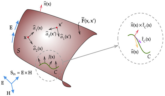
Figure 1.
General configuration of an electromagnetic surface receive system. (Left) Generic electromagnetic energy transfer system. An incoming generic near-field configuration , with Poynting vector interacts with the electromagnetic surface S. The port is modeled as a curve . The total current flowing through this port is the integral of all the components of the surface current density along the unit vector normal to C. In the diagram those normals are shown as black arrows. (Right) The details of the receive port model. The unit vector is normal to the page. The unit vector is the tangent to the curve C. The direction of the port current in general varies from one point on C to another, but we compute the port current using (5) as the total current flowing across C in the directions normal to the curve C, i.e., along the direction field .
The structure of this article unfolds as follows: In Section 2, we provide an overview of the foundational elements that constitute the theoretical model for electromagnetic surfaces, as proposed in this paper. Within this context, we present a concise yet comprehensive mathematical foundation regarding the concept of the electromagnetic current Green’s function of a surface, a fundamental notion that, despite its importance, remains relatively unfamiliar to many. Section 3 introduces the novel concept of near-field matching for the first time. This new operation generalizes the idea of discrete port matching in microwave circuit theory to a continuous domain of application, thanks to the rigorous formalism established in Section 2. As an application of the formulation outlined in Section 3, Section 4 offers insights into the wireless power transfer problem. In this section, we demonstrate that the capacity of electromagnetic energy coupling is fundamentally constrained by the geometry and material composition of the system. Finally, we end up with conclusions.
2. Theoretical Model
We work in the frequency domain, with being the radian frequency, where time representations of all dynamic quantities (fields and currents) are assumed to have the time-harmonic form , which is suppressed for convenience [22,37]. Consider a receiving surface S interacting with incident electromagnetic fields , where is the position vector; see Figure 1(left). The surface S is assumed to be an orientable smooth two-dimensional manifold with outward unit normal [24]. Our objective here is to describe a rigorous mathematical model allowing us to evaluate the potency of energy transfer from the interacting field to the interacting (receive) surface S. The model will assign specific degrees of freedom to characterize the production of signals (receive currents) representing power/energy capture. The electromagnetic field itself is assumed to be produced by another source, which might be close to S (near-field illumination) or far away (far-field illumination). However, in what follows, we will not take into consideration the details of this source. The radiation problem related to the production of illumination fields is a fundamentally different problem from the interaction with the receiving surface [39] (the former is the near-field focusing problem or antenna radiation problem [40,41,42].) Instead, we consider that the details of the illumination field are known or available to us. We then ask the following question: Starting from the initial data of a given near-field configuration , how could the shape and the electromagnetic responsitivity of the surface S be configured such that one may extract the maximal amount of power using the receiving system? To answer this question, we need to provide a precise mathematical model of the final received signal, which is an electric current (in Amps) extracted from the surface S.
Remark 1.
For the sake of simplicity, what follows will not take into account the magnetic field . This assumption is tantamount to considering that all receiving surfaces adhere to the perfect electric conductor (PEC) boundary condition [37,43]. In reality, one can incorporate the magnetic field by increasing the dimension (and hence complexity) of the Green’s operators of the problem [44]. Since this will not introduce fundamentally new ideas to our main objectives in this article, we leave the full extension to electric–magnetic field interactions to other publications, but see Appendix C for a rough outline of how this modification can be implemented.
The receive surface S might correspond to various physical scenarios, e.g., it can be the locus of the electromagnetic boundary conditions of an antenna systems [45,46,47], a metasurface [48,49,50], an information surface [51], or any functional structure whose operation depends on the capture of electromagnetic energy extracted from an illumination field. The total surface current density induced on S upon interaction with is denoted by (measured in A/m). Let be the three-dimensional current Green’s dyadic function tensor. Then, the surface current density can be computed in terms of the illumination field using the superposition formula [32,52]
The 3D tensor can be reduced to a 2D dimensional tensor using a system of local coordinate systems [43]. To do so, we exploit the differential structure, based on modeling S as a smooth 2-manifold, by deploying a system of orthonormal tangential vectors through the assignment
In other words, constitute an orthonormal basis for the tangent space of S based at [24]. Orthonormality is measured with respect to the Riemannian metric on S inherited from the embedding [53]. In terms of such a basis system, we may expand the current distribution as follows:
where are the vectorial projection maps. On the other hand, the current Green’s tensor will be written as [43]
where are the tensorial projection maps while is a tensor product. Note that this Green’s tensor is not a conventional tensor since it is not based on one point in S but is associated with both and . Technically, this tensor product should be defined in terms of the ambient Euclidean space into which the 2-manifold S is embedded [32].
Remark 2.
Strictly speaking, the elements of the Green’s tensor belong to the space of Schwartz distributions [29,54]. However, it can be shown that the tensor is the distributional limit of a sequence , where each term is a smooth complex-valued function [32,43,44]. In what follows, we simplify the notation by working with a “realization” of based on choosing a term with a sufficiently large n such that accurate estimation of the current on the S can be obtained. Proofs that for every given there exists such that the error in the estimated current is smaller than ϵ for all have been published in literature [32,43], with more details about computational aspects and experimental background [55,56,57].
In order to extract a load current from the receive surface system S, we must define a receive port model. In this paper, the port is defined as a curve , which can be either open or closed. The port current will then be defined as the total current flowing across C [37]. Let be the unit normal vector pointing away from S. From Figure 1(right), we may conclude that
where is the vector differential line element with being a unit vector tangential to both S and C at . Now since is normal to , the two-dimensional tangent space of the manifold S based at , it follows that . But, constitutes a basis for . Therefore, we can perform the expansion
where is the projection maps satisfying the condition
for all . Substituting (6) and (7) into (5) and making use of (3), we arrive at
The formula (8) expresses the total received current in terms of the surface current density and the geometrical structure of the port, where the latter is now to be encoded into two new problem-specific two-dimensional geometric vector field whose components are .
Our next theorem demonstrates that it is possible to bound irrespective of the geometric structure of the receive port.
Theorem 1.
Let be the port current for an arbitrary receive system , where S is the receive surface and C is the receive port. The real power extracted from the port C is , where R is the load resistance. Without loss of generality, we set . Then, the received power is bounded by
where the positive number , defined by
is the length of the port model curve C.
Proof.
Let us write the port geometric field as
Remark 3.
Even though in this paper, we assign the power capture measure to the total current flowing through a one-dimensional geometric structure, that of the smooth curve C, it should be noted that one can increase the “size” of C where power capture is evaluated. For example, in one extreme case, we can use space-filling curves. Space-filling curves are mathematical curves that can, in theory, completely fill a two-dimensional plane or higher-dimensional space [58,59]. These curves have the unique property of being continuous and surjective, meaning that they pass through every point in a given region without ever intersecting themselves. Therefore, since in the derivation based on the geometric model shown in Figure 1, there is no restriction on the port model other than the weak—and natural—condition , our mathematical formalism is general enough to deal with more complex scenarios, such as space-filling curves, where the area of power capture becomes a “one-dimensional approximation” of a continuous two-dimensional submanifold.
Remark 4.
One interesting feature of Theorem 1 is that the bound on is independent of the specific shape of the receive port C and instead depends only on the total length . This property will prove to be crucial in our derivation of an upper bound on the capacity of wireless power transfer systems, as shown below.
3. The Concept of Near-Field Matching
We now have the necessary tools to define the generalized concept of near-field matching. However, before providing the formal definition, let us first provide a physically intuitive motivation. In traditional circuit theory, an incident wave impinging on a port, where the latter is modeled as a discontinuity in an otherwise continuous one-dimensional structure (such as a waveguide, transmission line, or wire), would undergo reflection and transmission at the location of the port discontinuity [60]. In engineering practice, it is crucial to minimize multiple reflections caused by discontinuities in the longitudinal direction of wave propagation, and this is why port-matching techniques are widely used [61]. In such problems, the designer modifies the port structure, typically by inserting a matching section or circuit, such that the power delivered to the load after the port under consideration is maximized. However, this scenario is inherently discrete since circuit theory deals with a multiport structure where the number of ports is finite. Nevertheless, it is of general interest to investigate the much more complex situation depicted in Figure 1(left), where a continuous incident wave impinges on a continuous port distribution, namely the receive 2-manifold S. In this sense, there is a continuum of ports indexed by , with the field incident on the “th” port being the field . The corresponding problem of “generalized” matching would then consist of ensuring the simultaneous matching of all ports belonging to a continuum of locations extending over the entire surface S. We will call this process near-field matching since it is inspired by the concept of impedance matching in microwave circuit theory [62].
Definition 1.
(Near-field matching) Consider an illumination field interacting with a receive system whose current Green’s function is . This system will be represented mathematically by the quadruple . Let be the space of Schwartz distributions supported on the smooth manifold S [63]. (Based on Remark 2, this space can be replaced by the space of “realizations” of the current Green’s function , which is the function space of smooth dyadic tensors on ). Let be the function space of smooth vector fields tangential to S. The space of all possible 2-manifolds with total area will be denoted by . Similarly, the space of all geometric curves with length will be denoted by . Then, the problem of near-field matching is defined as the following optimization process:
under fixed or variable surface area and port contour length conditions of the forms and , respectively, maximum field condition and maximum current Green’s function norm (see Definition A1 for tensor norms.) The stars in the LHS of (13) indicate optimum values.
To put it differently, the objective is to configure the geometries of the corresponding receiving surface S and receiving port C in such a way that their topological and Riemannian characteristics align with the variation profile of the near-field illumination functional for all . This requires determining the appropriate Riemannian metric on S, say , and the tangent data on C (see (11)) that would lead to the maximum observable current signal at the port system C. Additionally, the functional forms of the field and current Green’s functions can be tailored to further optimize (maximize) the port current in conjunction with the geometric structures .
Our next goal is to establish fundamental limits that constrain the near-field matching optimization process described earlier. Specifically, we will demonstrate that there are restrictions on the relationship between the fields and the manifolds S and C defined on them. These constraints make the optimization process more complicated but also reveal that there are limits beyond which no optimal solutions can be found in principle. To obtain these limits, we need to estimate the sizes of various fields and operators involved. Our main strategy is to use a carefully chosen version of Young’s inequality for integral operators [34,35,36,64] to obtain an estimate of the received power in terms of all fields and geometries involved.
Motivated by Theorem 1, let us introduce the function space of Lebesgue square integrable vector fields on the 1-manifold C, whose norm is given by . Then, the relation (9) can be rewritten as
Our goal now is to derive an effective limit on maximal wireless power transfer by bounding the right-hand side of the inequality (14). To accomplish this, we will need to carefully employ various norms on suitable function spaces. Our primary tool for establishing a comparison measure between different functions will be Young’s inequality for kernel operators [34]. It is worth noting that the more well-known Young’s inequality for convolution kernels cannot be applied to our problem, as the current Green’s function in (1) is not spatially homogeneous. In other words, in general, the following situation holds:
In fact, in most practical scenarios, a typical lack of perfect spherical symmetry in S implies that (15) will hold for . [32,33,43] As a result of this obstacle, we will have to rely on the more general version of Young’s inequality, which is reviewed in Appendix A. In the statement of (A3) there, it is worth noting that the kernel need not be symmetric. The main result of this paper is presented in Theorem 2, where we derive the inequality (16). From this point onwards, we assume that all vector and dyadic tensor norms are to be interpreted in the sense of Definition A1 in Appendix B. This appendix also includes other important properties that will be utilized throughout the remainder of our discussion below.
Our main result is the following theorem.
Theorem 2.
Consider a near-field matching problem with the system . Then, the received power is bounded with the following estimate:
Proof.
Using (1) and (9), we compute
where the last inequality was obtained with the help of (A6), Theorem A2, Appendix B. We now note that this very last inequality in (17) is already given in a form suitable for the application of Young’s inequality (Appendix A). In particular, we choose , which satisfy (A2). Because of the equality (A10), Theorem A3, Appendix B, we can choose
4. Wireless Power Transfer Capacity and Its Upper Bound
As an application of the bound (16), we treat a specialized but important suboptimization problem separated from the more general near-field matching process of Definition 1, which is the matching of near field to the receive system under fixed current Green’s function . In this case, our objective is to use (16) to derive an upper bound on such a generic near-field optimization problem. To do so, we first need to propose a suitable measure to characterize the efficacy of the process of wireless energy transfer. Note that standard measures and techniques such as those found in the literature cannot be directly used in our case illustrated in Figure 1 because we start with a given tangential near field distribution , not an input port. We also do not calculate Poynting vector in this problem since the interaction only occurs with the electric field [43,52]. Most available measures use port-to-port coupling or transfer ratio, which defines the efficacy of the system in terms of energy/power efficiency while the maximal power transfer is established via a circuit-type conjugate impedance-based maximum power transfer theorem [19,65,66,67]. In the following definition, we introduce an intuitive measure suitable for field quantities like those appearing in Figure 1. The key idea is that, as the total area of the capture surface S and length of the receive port C increase, the net achieved power transfer will increase too. Therefore, our field-theoretic measure must use spatial averages of field intensities. These averages can be compared with the corresponding port-to-port theories available in literature in the sense that we average a “continuum of ports” distributed in S to produce an effective single port, and so on.
Definition 2
(Electromagnetic power transfer capacity). We define the capacity of the system as the received power per unit port square length per the square of the average value of the illumination tangential field on the surface S. Mathematically, we write this quantity as
where R is load resistance and
is the total area of S.
Remark 5.
The quantity then has units of so it is physically like a transfer conductance connecting average field intensity over the surface S and current intensity (power) over the port C. Physically, we may interpret the numerator of (20) as the average value of the square of the current density over the entire port system C. The denominator is the average value of the field intensity over the entire surface S. Therefore, the capacity measures the relative ability of the receive system to extract power from the incoming near field since the ratio characterizes how much current intensity is produced (per position on receive port) with respect to incident field intensity (per position on receive surface).
Using the definition (20) in (16), we immediately conclude that
where we set . We may derive a looser bound by noting that
where
while we note that the latter maximum operation exists because is compact [68]. Consequently, (22) becomes
However, the bound in (22) is tighter than (24) because the former includes detailed information on how the values of the current Green’s function are distributed with respect to the Riemannian geometric structure of the problem.
The relation (22) constitutes a fundamental upper bound on the capacity of the receive system . It shows that capacity is proportional to the square of the receive system area and inversely proportional to the port length . Physically, this upper bound sets a fundamental limit on what optimization (via near field matching) can achieve relative to a given current Green’s function . Indeed, the inequality (22) states that no matter how we shape the geometry of the receive system’s surface or port, the capacity achievable of the power transfer system is bounded from above by the distribution of values of the current Green’s function (the electromagnetic responsitivity of the surface). Some of the major applications of our exact bound could include studies attempting to understand the process of electromagnetic energy transfer in random environments where one attempts to derive efficiency measures describing how the system would perform in the average statistical scenario [19]. Within this context, it is possible to build a random field-theoretic model by assuming that both the illumination field and the current Green’s function become random fields on the manifolds S and , respectively [25]. In this sense, fundamental universal inequalities such as (16) and (22) can play an essential role in designing strategies for the simulation of such random field-based wireless power scenarios [69].
5. Conclusions
Wireless power transfer and the understanding of electromagnetic energy coupling are essential for the efficient operation of industrial and sensor applications. By maximizing the received signal and enabling the efficient transfer of power, wireless power transfer improves the performance and sustainability of the energy infrastructure, enabling the development of modern energy-efficient societies. While there had been significant progress in solving practical problems related to wireless energy transfer, there is a need for more research focused on the general abstract form of the problem while explicating its fundamental mathematical structure. By adopting such a more abstract approach while considering generic field-receiver interaction scenarios, universal solutions could be developed that applied to a wide range of applications and helped advance the field of wireless energy transfer. This work provided a rigorous theoretical framework for understanding and optimizing energy transfer and exchange in complex near-field electromagnetic systems, with potential applications in areas such as wireless power transfer and electromagnetic sensing. Our key innovation was using the current Green’s function of a surface to theoretically describe how a generic smooth 2-manifold interacts with an arbitrary electromagnetic near field such that maximal power extraction can be achieved and then utilizing Young’s inequality for an integral operator to derive exact upper bounds on the received current valid for arbitrary geometries and incoming field profiles. The obtained bounds were applied to the generalized problem of near-field matching, where the continuous spatial profile of the field is matched to both the electromagnetic and geometric structure of the receive surface. We found that a proper measure of the efficacy of the wireless power transfer system, the capacity, is bounded by a functional that depends only on the current Green’s function and is proportional to the cube of the receive surface area. The current theoretical investigation and the universal bounds approach could still be further expanded in future work. For example, the single-electric-field formalism presented above could be generalized to deal with interactions including both electric and magnetic fields together, a useful feature to have in the case of mixed PEC-dielectric electromagnetic boundary conditions [44]. Only the size and complexity of the Greens functions would increase but the basic core idea could still be applied to this problem.
Funding
This research received no external funding.
Data Availability Statement
Not applicable.
Conflicts of Interest
The author declares no conflict of interest.
Appendix A. Young Inequality for Integral Kernel Operators
The Young inequality in Fourier analysis is an important result that relates the size of a function and its Fourier transform [34,35,36,64]. Specifically, it gives an estimate on the -norm of the Fourier transform of a function in terms of the -norm of the function itself, with some restrictions on the p and q exponents (see below). This result is often used in the study of partial differential equations, harmonic analysis, and related areas of mathematics [36,70]. A simple version of the Young inequality for integral kernel operators can be stated as follows.
Theorem A1
(Young’s inequality for integral operators). Let be a measurable function on , where are measurable spaces. Let T be the integral operator defined by
for all . Then, for such that
we have the following estimate:
where denotes the norm of and denotes the norm of . The constant B is chosen such that the following two conditions hold:
Appendix B. Norms of Tensors and Some of Their Properties
Definition A1.
The norm of a complex vector , denoted by , is defined in the usual manner as . For a dyad , the norm in this paper is defined as the Frobenius norm of the matrix representation with respect to any chosen basis
All these norms are independent of the chosen basis [71].
Theorem A2.
Let and be an arbitrary vector and tensor fields on S and , respectively, with norms defined as per Definition A1. Then, for all , we have
Proof.
We introduce the compact vector notation:
In terms of this notation, the multiplication of the current Green’s function tensor (4) with the electric field can be written as
Consequently, we find
Theorem A3.
For all reciprocal electromagnetic surfaces such that , we have
Appendix C. Treatment of H Fields
In the domain of electromagnetic systems, a typical scenario involves the presence of both perfectly electrically conducting (PEC) objects and dielectric subsystems. In such inherently intricate configurations, the interactions with magnetic fields become crucial. To effectively address these mixed conducting/dielectric scenarios, the most suitable formalism revolves around the utilization of appropriate surface equivalence theorems [37]. In this context, we offer a succinct overview of how the formalism presented in our current work can be extended to encompass interactions with magnetic fields within wireless energy transfer systems. Let and represent the electric and magnetic currents as defined in the surface equivalence theorem formulation [37] of the given problem. The generalized current Green’s function formalism allows us to compute the induced surface currents using the following Green’s function expression:
where , , , and are the electric/electric, electric/magnetic, magnetic/electric, and magnetic/magnetic Green’s function dyads, respectively. For complete information on how these dyadic functions are defined, including their various compact support regions within the surface-equivalent configuration of boundary conditions, see [44]. We now work in parallel to Definition A1 and introduce the following norms for the dyadic and vector arrays appearing in (A13).
Definition A2.
The norm of a complex vector array is defined as
For an array of dyadic complex tensors, the norm in this paper is defined as the generalization of the Frobenius norm of the matrix representation with respect to any chosen basis:
where is defined as in Definition A1. Again, it is easy to show that all these norms are independent of the chosen basis.
Finally, based on Definition A2 and the formula (A13), one can apply the same methods developed in this paper in order to derive upper bounds on energy transfer for mixed dielectric-conducting systems.
References
- Sun, T.; Xie, X.; Wang, Z. Wireless Power Transfer for Medical Microsystems; Springer: New York, NY, USA, 2013. [Google Scholar]
- Zhang, X.; Zhu, C.; Song, H. Wireless Power Transfer Technologies for Electric Vehicles, 1st ed.; Springer: Singapore, 2022. [Google Scholar]
- Yilmaz, G.; Dehollain, C. Wireless Power Transfer and Data Communication for Neural Implants, 1st ed.; Springer International Publishing: Cham, Switzerland, 2017. [Google Scholar]
- Nikoletseas, S.; Yang, Y.; Georgiadis, A. (Eds.) Wireless Power Transfer Algorithms, Technologies and Applications in Ad Hoc Communication Networks, 1st ed.; Springer International Publishing: Cham, Switzerland, 2016. [Google Scholar]
- Jayakody, D.N.K.; Sharma, S.K.; Chatzinotas, S. Introduction, recent results, and challenges in wireless information and power transfer. In Wireless Information and Power Transfer: A New Paradigm for Green Communications; Springer International Publishing: Cham, Switzerland, 2018; pp. 3–28. [Google Scholar]
- Kim, H.; Hirayama, H.; Kim, S.; Han, K.J.; Zhang, R.; Choi, J. Review of Near-Field Wireless Power and Communication for Biomedical Applications. IEEE Access 2017, 5, 21264–21285. [Google Scholar] [CrossRef]
- Khan, T.A.; Yazdan, A.; Heath, R.W. Optimization of Power Transfer Efficiency and Energy Efficiency for Wireless-Powered Systems With Massive MIMO. IEEE Trans. Wirel. Commun. 2018, 17, 7159–7172. [Google Scholar] [CrossRef]
- Liu, G.; Sun, Z.; Jiang, T. Joint Time and Energy Allocation for QoS-Aware Throughput Maximization in MIMO-Based Wireless Powered Underground Sensor Networks. IEEE Trans. Commun. 2019, 67, 1400–1412. [Google Scholar] [CrossRef]
- Arnitz, D.; Reynolds, M.S. MIMO Wireless Power Transfer for Mobile Devices. IEEE Pervasive Comput. 2016, 15, 36–44. [Google Scholar] [CrossRef]
- Imura, T. Wireless Power Transfer, 1st ed.; Springer: Singapore, 2020. [Google Scholar]
- Perez-Nicoli, P.; Silveira, F.; Ghovanloo, M. Inductive Links for Wireless Power Transfer, 1st ed.; Springer Nature: Cham, Switzerland, 2021. [Google Scholar]
- Zhong, W.; Xu, D.; Hui, R.S.Y. Wireless Power Transfer: Between Distance and Efficiency, 1st ed.; Springer: Singapore, 2020. [Google Scholar]
- Ng, D. Wireless Information and Power Transfer—Theory and Practice; Wiley-IEEE, Wiley-Blackwell: Hoboken, NJ, USA, 2019. [Google Scholar]
- Zhang, R.; Ho, C.K. MIMO Broadcasting for Simultaneous Wireless Information and Power Transfer. IEEE Trans. Wirel. Commun. 2013, 12, 1989–2001. [Google Scholar] [CrossRef]
- Kurs, A.; Karalis, A.; Moffatt, R.; Joannopoulos, J.D.; Fisher, P. Wireless power transfer via strongly coupled magnetic resonances. Science 2007, 317, 83–86. [Google Scholar] [CrossRef]
- Öner, I.H.; David, C.; Querebillo, C.J.; Weidinger, I.M.; Ly, K.H. Electromagnetic Field Enhancement of Nanostructured TiN Electrodes Probed with Surface-Enhanced Raman Spectroscopy. Sensors 2022, 22, 487. [Google Scholar] [CrossRef]
- Sanz-Fernandez, J.J.; Mateo-Segura, C.; Cheung, R.; Goussetis, G.; Desmulliez, M.P.Y. Near-field enhancement for infrared sensor applications. J. Nanophotonics 2011, 5, 053510. [Google Scholar] [CrossRef]
- Brown, W.C. The history of power transmission by radio waves. IEEE Trans. Microw. Theory Tech. 1984, 32, 1230–1242. [Google Scholar] [CrossRef]
- Rossi, M.; Stockman, G.J.; Rogier, H.; Vande Ginste, D. Stochastic Analysis of the Efficiency of a Wireless Power Transfer System Subject to Antenna Variability and Position Uncertainties. Sensors 2016, 16, 1100. [Google Scholar] [CrossRef]
- So, M.C.; Wiederrecht, G.P.; Mondloch, J.E.; Hupp, J.T.; Farha, O.K. Metal-organic framework materials for light-harvesting and energy transfer. Chem. Commun. 2015, 51, 3501–3510. [Google Scholar] [CrossRef] [PubMed]
- Ilinskii, Y.A.; Keldysh, L. Electromagnetic Response of Material Media; Springer: New York, NY, USA, 1994. [Google Scholar]
- Felsen, L. Radiation and Scattering of Waves; IEEE Press: Piscataway, NJ, USA, 1994. [Google Scholar]
- Ishimaru, A. Wave Propagation and Scattering in Random Media; Oxford University Press: New York, NY, USA, 1997. [Google Scholar]
- Lee, J. Introduction to Smooth Manifolds; Springer: New York, NY, USA; London, UK, 2012. [Google Scholar]
- Adler, R.J.; Taylor, J. Random Fields and Geometry; Springer: New York, NY, USA, 2007. [Google Scholar]
- Schwarz, A.S. Topology for Physicists; Springer: Berlin/Heidelberg, Germany; New York, NY, USA, 1994. [Google Scholar]
- Hirsch, M. Differential Topology; Springer: New York, NY, USA, 1976. [Google Scholar]
- Kelley, J. General Topology; Dover Publications, Inc.: Mineola, NY, USA, 2017. [Google Scholar]
- Hassani, S. Mathematical Physics: A Modern Introduction to Its Foundations; Springer: Cham, Switzerland, 2013. [Google Scholar]
- Munkres, J. Topology; Pearson: New York, NY, USA, 2018. [Google Scholar]
- Zeidler, E. Applied Functional Analysis: Applications to Mathematical Physics; Springer: Berlin/Heidelberg, Germany, 1995. [Google Scholar]
- Mikki, S.; Antar, Y. The antenna current Green’s function formalism—Part I. IEEE Trans. Antennas Propag. 2013, 9, 4493–4504. [Google Scholar] [CrossRef]
- Mikki, S. The Antenna Spacetime System Theory of Wireless Communications. Proc. R. Soc. 2019, 475, 20180699. [Google Scholar] [CrossRef]
- Sogge, C.D. Fourier Integrals in Classical Analysis; Cambridge University Press: Cambridge, UK, 1993. [Google Scholar]
- Stein, E.M. Harmonic Analysis: Real-Variable Methods, Orthogonality, and Oscillatory Integrals; Princeton University Press: Princeton, NJ, USA, 1993. [Google Scholar]
- Stein, E.M.; Weiss, G. Introduction to Fourier Analysis on Euclidean Spaces; Princeton University Press: Princeton, NJ, USA, 1971. [Google Scholar]
- Van Bladel, J.G. Electromagnetic Fields; Wiley-Intersience: Hoboken, NJ, USA, 2007. [Google Scholar]
- Schelkunoff, S.A. A Mathematical Theory of Linear Arrays. Bell Syst. Tech. J. 1943, 22, 80–107. [Google Scholar] [CrossRef]
- Schelkunoff, S.A. Theory of antennas of arbitrary size and shape. Proc. IEEE 1984, 72, 1165–1190. [Google Scholar] [CrossRef]
- Hansen, T.; Yaghjian, A.D. Plane-Wave Theory of Time-Domain Fields: Near-Field Scanning Applications; IEEE Press: New York, NY, USA, 1999. [Google Scholar]
- Mikki, S.; Antar, Y. A Theory of Antenna Electromagnetic Near Field—Part I. IEEE Trans. Antennas Propag. 2011, 59, 4691–4705. [Google Scholar] [CrossRef]
- Mikki, S.; Antar, Y.M.M. A Theory of Antenna Electromagnetic Near Field—Part II. IEEE Trans. Antennas Propag. 2011, 59, 4706–4724. [Google Scholar] [CrossRef]
- Mikki, S.; Antar, Y. New Foundations for Applied Electromagnetics: The Spatial Structure of Fields; Artech House: London, UK, 2016. [Google Scholar]
- Mikki, S. Generalized Current Green’s Function Formalism for Electromagnetic Radiation by Composite Systems. Prog. Electromagn. Res. 2020, 87, 171–191. [Google Scholar] [CrossRef]
- Balanis, C.A. Antenna Theory: Analysis and Design, 4th ed.; Wiley Inter-Science: Hoboken, NJ, USA, 2015. [Google Scholar]
- Schelkunoff, S.A.; Friss, H.T. Antennas: Theory and Practice; Chapman & Hall: London, UK; New York, NY, USA, 1952. [Google Scholar]
- Cloude, S. An Introduction to Electromagnetic Wave Propagation & Antennas; Springer: New York, NY, USA, 1996. [Google Scholar]
- Holloway, C.L.; Kuester, E.F.; Gordon, J.A.; O’Hara, J.; Booth, J.; Smith, D.R. An Overview of the Theory and Applications of Metasurfaces: The Two-Dimensional Equivalents of Metamaterials. IEEE Antennas Propag. Mag. 2012, 54, 10–35. [Google Scholar] [CrossRef]
- Wu, Q.; Zhang, R. Towards Smart and Reconfigurable Environment: Intelligent Reflecting Surface Aided Wireless Network. IEEE Commun. Mag. 2020, 58, 106–112. [Google Scholar] [CrossRef]
- Tang, W.; Dai, J.Y.; Chen, M.Z.; Wong, K.K.; Li, X.; Zhao, X.; Jin, S.; Cheng, Q.; Cui, T.J. MIMO Transmission Through Reconfigurable Intelligent Surface: System Design, Analysis, and Implementation. IEEE J. Sel. Areas Commun. 2020, 38, 2683–2699. [Google Scholar] [CrossRef]
- Cui, T.; Tang, W.X.; Yang, X.M.; Mei, Z.L.; Jiang, W.X. Metamaterials: Beyond Crystals, Noncrystals, and Quasicrystals; CRC Press: Boca Raton, FL, USA, 2016. [Google Scholar]
- Mikki, S.; Antar, Y. On the Fundamental Relationship Between the Transmitting and Receiving Modes of General Antenna Systems: A New Approach. IEEE Antennas Wirel. Propag. Lett. 2012, 11, 232–235. [Google Scholar] [CrossRef]
- Burns, K.; Gidea, M. Differential Geometry and Topology: With a View to Dynamical Systems; CRC Press: Boca Raton, FL, USA, 2005. [Google Scholar]
- Appel, W. Mathematics for Physics and Physicists; Princeton University Press: Princeton, NJ, USA, 2007. [Google Scholar]
- Kim, Y.; Kim, H.; Bae, K.; Park, J.; Myung, N. A Hybrid UTD-ACGF Technique for DOA Finding of Receiving Antenna Array on Complex Environment. IEEE Trans. Antennas Propag. 2015, 63, 5045–5055. [Google Scholar] [CrossRef]
- Yang, S.; Kim, Y.; Jo, H.; Myung, N. Alternative Method for Obtaining Antenna Current Green’s Function Based on Infinitesimal Dipole Modeling. IEEE Trans. Antennas Propag. 2019, 67, 2583–2590. [Google Scholar] [CrossRef]
- Mikki, S.; Antar, Y. The antenna current Green’s function as an alternative method to conventional full-wave analysis solvers: An outline. In Proceedings of the 2015 IEEE MTT-S International Conference on Numerical Electromagnetic and Multiphysics Modeling and Optimization (NEMO), Ottawa, ON, Canada, 11–14 August 2015; pp. 1–3. [Google Scholar]
- Cannon, J.W.; Thurston, W.P. Group invariant Peano curves. Geom. Topol. 2007, 11, 1315–1355. [Google Scholar] [CrossRef]
- Sagan, H. Space-Filling Curves; Universitext; Springer: New York, NY, USA, 1994. [Google Scholar]
- Felsen, L.B.B. Electromagnetic Field Computation by Network Methods; Springer: Berlin/Heidelberg, Germany, 2010. [Google Scholar]
- Collin, R. Foundations for Microwave Engineering; IEEE Press: New York, NY, USA, 2001. [Google Scholar]
- Collin, R.E. Field Theory of Guided Waves; Wiley-IEEE Press: Hoboken, NJ, USA, 1991. [Google Scholar]
- Gelfand, I.; Vilenkin, N. Generalized Functions: Volume 4; Academic Press: New York, NY, USA; London, UK, 1964. [Google Scholar]
- Okikiolu, G.O. On inequalities for integral operators. Glasg. Math. J. 1970, 11, 126–133. [Google Scholar] [CrossRef]
- Machnoor, M.; Lazzi, G. Wireless Power Transfer: Types of Reflected Impedances and Maximum Power Transfer Theorem. IEEE Antennas Wirel. Propag. Lett. 2020, 19, 1709–1713. [Google Scholar] [CrossRef]
- Kiani, M.; Ghovanloo, M. The Circuit Theory Behind Coupled-Mode Magnetic Resonance-Based Wireless Power Transmission. IEEE Trans. Circuits Syst. Regul. Pap. 2012, 59, 2065–2074. [Google Scholar] [CrossRef]
- Warnick, K.F.; Gottula, R.B.; Shrestha, S.; Smith, J. Optimizing Power Transfer Efficiency and Bandwidth for Near Field Communication Systems. IEEE Trans. Antennas Propag. 2013, 61, 927–933. [Google Scholar] [CrossRef]
- Godement, R. Analysis I: Convergence, Elementary Functions; Springer: Berlin, Germany; New York, NY, USA, 2004. [Google Scholar]
- Hristopulos, D.T. Random Fields for Spatial Data Modeling, 1st ed.; Springer: Dordrecht, The Netherlands, 2020. [Google Scholar]
- Duoandikoetxea, J. Fourier Analysis; Graduate Studies in Mathematics; American Mathematical Society: Providence, RI, USA, 2011; Volume 29. [Google Scholar]
- Horn, R.; Johnson, C.R. Matrix Analysis; Cambridge University Press: New York, NY, USA, 2012. [Google Scholar]
- Mikki, S.; Antar, Y. The antenna current Green’s function formalism—Part II. IEEE Trans. Antennas Propag. 2013, 9, 4505–4519. [Google Scholar] [CrossRef]

Disclaimer/Publisher’s Note: The statements, opinions and data contained in all publications are solely those of the individual author(s) and contributor(s) and not of MDPI and/or the editor(s). MDPI and/or the editor(s) disclaim responsibility for any injury to people or property resulting from any ideas, methods, instructions or products referred to in the content. |
© 2023 by the author. Licensee MDPI, Basel, Switzerland. This article is an open access article distributed under the terms and conditions of the Creative Commons Attribution (CC BY) license (https://creativecommons.org/licenses/by/4.0/).