Abstract
In classical survival analysis, it is assumed that all the individuals will experience the event of interest. However, if there is a proportion of subjects who will never experience the event, then a standard survival approach is not appropriate, and cure models should be considered instead. This paper deals with the problem of adapting a machine learning approach for classical survival analysis to a situation when cure (i.e., not suffering the event) is a possibility. Specifically, a brief review of cure models and recent machine learning methodologies is presented, and an adaptation of machine learning approaches to account for cured individuals is introduced. In order to validate the proposed methods, we present an extensive simulation study in which we compare the performance of the adapted machine learning algorithms with existing cure models. The results show the good behavior of the semiparametric or the nonparametric approaches, depending on the simulated scenario. The practical utility of the methodology is showcased through two real-world dataset illustrations. In the first one, the results show the gain of using the nonparametric mixture cure model approach. In the second example, the results show the poor performance of some machine learning methods for small sample sizes.
Keywords:
censored data; cure rate; deep learning; mixture cure models; simulation; system reliability MSC:
62N02
1. Introduction to Survival Analysis
Survival analysis is a branch of statistics whose object of study is the elapsed time until an event of interest. Depending on its application, survival analysis has been widely used in many areas: engineering (time to failure of a machine), economics (duration of unemployment), medicine (time to death due to a specific medical condition), etc. A relevant characteristic in survival analysis is that the event of interest does not always occur during the follow-up period or that the failure time cannot be exactly defined. This absence of information leads to the concept of censoring. The main challenge in survival analysis is how to handle censored data. Specifically, there are two common cases of censoring. On the one hand, point censoring occurs when the individual does not experience the event within the study period. Two types of point censoring can be defined: right censoring (the event of interest is experienced after the end of study, since it is not possible to follow the individuals for an infinite period of time) and left censoring (it is known that the failure occurred prior to the start of follow-up). On the other hand, an individual is interval censored if it is known that the event occurred between two times, but it is not possible to determine the exact failure time. In this paper, we focus on the most common censoring case: point censoring and, specifically, right censoring (see, among others, refs. [1,2,3,4]).
In standard survival analysis, it is assumed that the individuals, if they could be followed an infinite amount of time, would all experience the event of interest. Nevertheless, there might be some situations in which a group of individuals will never suffer the event, no matter how long they are followed. For example, for a dataset related to cancer patients, if the event is death due to cancer, it is known that not all the subjects will suffer the event. In statistics, this group of long-term survivors is considered as cured. It is important to highlight that the term cure does not mean the absence of illness: it refers to the fact that the individuals will not suffer the event of interest. In order to accommodate the group of cured individuals, classical survival methods have been extended to cure models.
Although the first cure models were proposed in the 1950s, these models have received increasing attention in the last decades (see, between others, [3,5]). This is due, partly, to the effectiveness of current cancer treatments: the proportion of patients who are cured (or who, at least, survive for a long time) is increasing over time. In such a context, a classical survival approach is not appropriate and cure models should be considered.
Recent works pointed out that machine learning algorithms, especially deep learning (DL) algorithms, are a solid choice to compute the survival estimation in classic survival scenarios [6,7,8,9], establishing the state-of-the-art solutions in this field. However, little has been achieved in computing the cure fraction, which is usually referred to as the cure rate (see, among others, ref. [10,11,12]).
In this paper, we compare different techniques to compute the cure fraction. Specifically, we consider a mixture cure model approach, and we focus on how machine learning can be combined with a cure model framework to estimate the cure rate. The main contributions of this paper are twofold:
- We propose to adapt the nonparametric mixture cure model approach by [13] to ML methods. We show that all state-of-the-art ML techniques can be used to compute the cure rate by placing a slight modification in the algorithms.
- An extensive study is conducted, in which we compare the performance of the adapted ML algorithms with existing cure models. Furthermore, a real data application is also presented, in which we show the gain of using some of the proposed methods in specific situations and some drawbacks to take into account when working with small sample sizes.
The paper is organized as follows: in Section 2, we review the recent developments in cure models; in Section 3, we describe the state-of-the-art of machine learning approaches for classical survival analysis and propose a nonparametric adaptation to account for cured individuals; in Section 4, we conduct an extensive simulation study to compare both methodologies, which are applied to two medical datasets in Section 5.1. In Section 6, we comment the results, offering some advises related to how and when one should use the tested methods. Finally, in Section 7, we detail some conclusions and future research lines.
2. Cure Models
Cure models consider a proportion of subjects who will never experience the event, that is, the cure fraction.
These models are mainly classified in two groups: non-mixture cure models (NMCMs) and mixture cure models (MCMs). NMCMs, also known as proportional hazard (PH) or promotion time cure models, were introduced by [14] and deeply studied in [15,16]. In the literature, there is a wide variety of parametric (see [17,18,19], among others), semiparametric (see [20,21,22,23]), and nonparametric NMCM approaches (see [24]). One disadvantage of the NMCM approach is that it forces the covariates to have the same influence on all the individuals (those who will experience the event and those who will not). In this work, we focus on MCMs, which consider the survival function as a mixture of two groups of subjects: the susceptible group and the cured group. This feature allows the covariates to have different influence on both sets of observations.
We will use the standard notation. Let Y be the time to occurrence of the event and C the censoring time. The survival function, S, is defined as:
In classical survival analysis, . However, if there is a proportion of cured subjects, then
Due to random right censoring, the variable Y will not always be observed. Therefore, for each individual, we have the pair , where is the time until an individual either experiences the event of interest or their follow-up period ends, and is the uncensoring indicator. A sample is a collection of observations: , independent and identically distributed (i.i.d.) copies of the random vector . Note that, for , if corresponds to an uncensored observation, then and . Otherwise, and .
One of the main goals in survival analysis is to estimate the density and distribution (or survival) functions of Y. In the literature, Ref. [25] introduced the nonparametric maximum-likelihood estimator of the survival function in presence of censoring, also known as the product-limit (PL) estimator:
where is the corresponding uncensoring indicator concomitant of and are the ordered ’s. In addition, note that if , then . Later, ref. [26] proposes a generalization of the Kaplan–Meier estimator, which allows the presence of covariates:
where are Nadaraya–Watson weights with , the rescaled kernel with bandwidth . Note that is the covariate concomitant of .
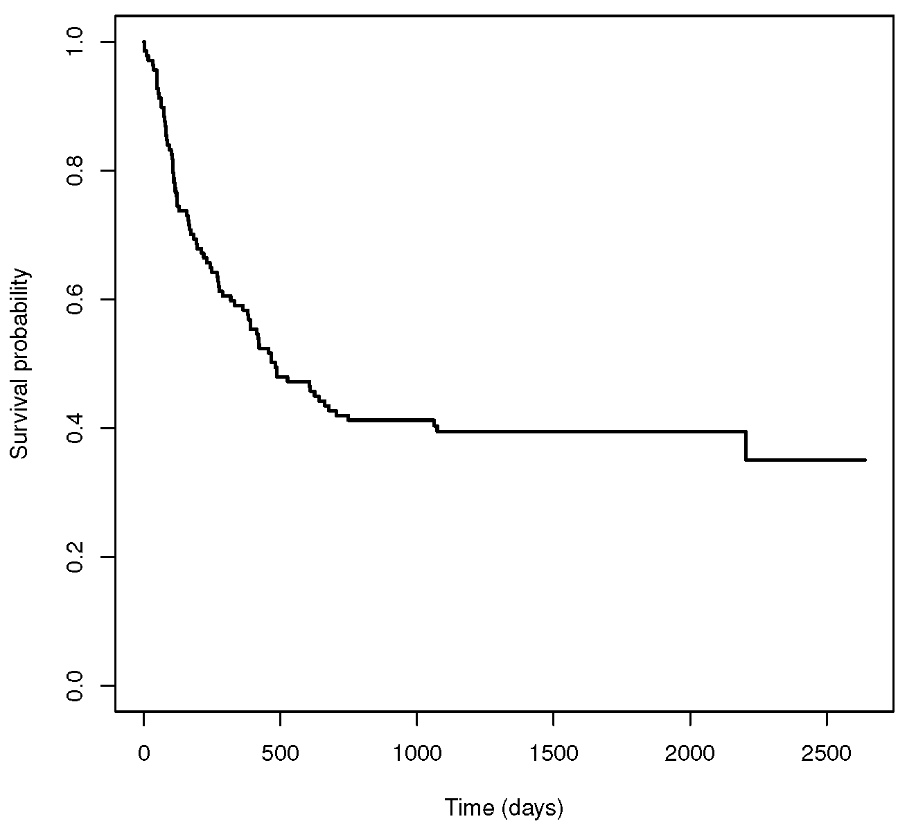
In order to illustrate the necessity of cure models, let us introduce a real example in which we do not consider the cure possibility. We work with a dataset related to 137 bone marrow transplant patients (see [27,28]). The dataset is described in detail in Section 5.2. Figure 1 shows the Kaplan–Meier estimator for the survival function for the complete dataset, . We can observe that the survival curve of has a plateau at the end of the study. In the literature (see [13,29]), this non-zero asymptote is taken as an estimator of the cure rate. Specifically, the estimated cure probability is 0.35 for this dataset. Since a standard survival model does not take into account the proportion of individuals who are cured, it is not an appropriate way to analyze the data. On the contrary, a cure model may be a suitable alternative.

Figure 1.
Standard survival function related to the bone marrow transplant dataset.
Therefore, to account for the cure fraction, let us define as a binary variable, with if the individual belongs to the susceptible group and if the individual belongs to the cured group. Note that is partially observed, since it is not possible to distinguish between those susceptible individuals that are censored and those observations of cured individuals. In addition, let be the conditional probability of not being cured:
In the literature (see [13,29]), the cure rate is estimated as follows:
Furthermore, the conditional survival function for the uncured population, referred to as latency, is defined as
Then, the MCM can be written as
Note that, in Equation (2), is the cure rate and is the latency, which corresponds to the subjects who will suffer the event of interest. Since the MCM approach allows the covariates to have different influence on cured and uncured individuals, let us define Z as a covariate which only influences the insusceptible subjects. Therefore, the MCM in Equation (2) can be written as
Depending on the assumptions established for either the latency or the cure rate, there are parametric, semiparametric, and nonparametric approaches of MCMs. A thorough review of the most relevant proposals in the literature can be found in [3,5], among others.
2.1. Parametric MCM
The first approaches in MCM were introduced by [30] in a study related to the relapse of mouth cancer patients. The cure rate was considered as a constant and the latency was modeled as a lognormal distribution with independence to any covariate. Later, ref. [31] delved into Boag’s approach and considered an exponential model for the latency, also with independence of covariates.
The first MCMs considering the influence of covariates were developed by [32]. They proposed to estimate the cure rate with a logistic function and the latency with a Weibull distribution. One decade later, ref. [33] introduced the accelerated failure time (AFT) model for the latency. This model, which was later studied by [34], assumes the presence of covariates with fixed and multiplicative effects. Another example of a parametric MCM was developed by [35]. They considered a parametric approach to study the impact of several variables on the survival time of patients with follicular lymphomas. In addition, ref. [36] proposed a pseudo-residual model to assess the fit of the survival regression in the non-cured fraction for mixture cure models and applied their method to a dataset related to a smoking cessation drug trial. More recently, ref. [37] provided introduced a multivariate mixture cure rate model based on the Chen probability distribution to model recurrent event data in the presence of cured individuals. Regarding goodness-of-fit tests, ref. [38] introduced a method to test whether the cure rate, as a function of the covariates, satisfies a certain parametric model. Furthermore, in a context with interval-censored data, ref. [39], developed a parametric but flexible statistical model and ref. [40] proposed a goodness-of-fit test which deals with partly interval-censored data.
2.2. Semiparametric MCM
Due to the fact that the effects of the covariates on the mixture cure model cannot always be well approximated using a parametric method, semiparametric models arose. These models provide considerably more flexibility than the parametric approaches. In the literature, most semiparametric models attribute flexibility to latency, whereas the cure rate is modeled parametrically (usually, assuming a logistic function). For example, ref. [41] proposed an estimation procedure for a parametric cure rate that relies on a preliminary smooth estimator and is independent of the semiparametric model assumed for the latency.
One category in this group includes the AFT models, which consist of a semiparametric adaptation for the latency of the AFT parametric models (see [42,43,44] among others). Specifically, a logistic regression is considered for the cure rate and the latency is determined by an AFT regression model with unspecified error distribution and estimated via EM methods. The EM algorithm was also considered in this context by [45] to model the effect of the covariates on the failure time of uncured individuals. Another category in semiparametric MCMs contains flexible models [46]. These models consider either the probit or the log-log distributions to infer the cure rate, and the EM algorithm and maximum-likelihood criterion to estimate the parameters. Furthermore, a third category includes the semiparametric approaches based on splines (see [47,48,49], among others). More recently, ref. [50] proposed a semiparametric MCM approach related to single-index structures, which could be considered as a fourth category in this section. These models are defined with a nonparametric form for the latency and semiparametric methods for the cure rate.
In spite of adding certain flexibility in some terms of the model, semiparametric approaches still have the disadvantage of restricting some functions to a previously defined form, which may not be fulfilled in many realistic cases and lead to estimation errors.
2.3. Nonparametric MCM
Very few papers exist that use a completely nonparametric view. The first nonparametric MCMs were introduced by [51]. Specifically, these authors proposed to estimate the cure rate as the height of the non-zero asymptote in the survival curve. However, they did not consider the effect of covariates in the model. In order to deal with this challenge, ref. [52] took into account discrete variables.
The main leap for the development of nonparametric MCMs was carried out by [13], who proposed a nonparametric cure rate estimator which can handle both types of continuous and discrete covariates. In [29], this estimator was deeply studied, and a nonparametric approach for the latency was proposed. Note that, in a nonparametric context, the choice of the bandwidth is of primary importance, since it controls the trade-off between bias and variance. A plug-in bandwidth selector which can be used in this context is the one introduced by [53]. Another option to select the smoothing parameter is with a bootstrap approach. A bootstrap bandwidth selection method for the cure rate and for the latency estimators has been proposed in [29,54], respectively. It is important to highlight that, due to the curse of dimensionality, the completely nonparametric models in the literature which are implemented in R can only handle a univariate continuous covariate [55,56]. Therefore, testing the effect of a covariate is a relevant aspect in regression analysis since the number of potential covariates to be included in the model can be extremely large. A nonparametric covariate hypothesis test for the cure rate, which can be applied to continuous, discrete, and qualitative covariates, has been introduced by [57].
3. Machine Learning Techniques Applied to Survival Analysis
Over the past years, hand in hand with computational capabilities, machine learning has been evolving and improving its ability to confront traditional regression and classification problems. The continued improvement made machine learning community interested in adapting these methodologies to other branches, including survival analysis. The main challenge researchers deal with is the presence of censored data (a rare feature in traditional machine learning problems).
In the literature, there are multiple complex machine learning models which take into account the presence of censored observations and study the event of interest over time [58]. Generally speaking, four machine learning approaches have been used for survival analysis:
- Survival Trees: the tree-like approaches were the first machine learning models successfully used to handle censored data. Similarly to other tree-like algorithms, the main idea is to split the data according to the similarity among observations, grouping similar data in the same branches while keeping the different data apart. The key of these models is the splitting criterion, which can be classified into two categories: those that minimize within-node homogeneity [59,60,61,62,63,64] and those that maximize between-node heterogeneity [65,66,67]. Amongst the last group, the more recent Random Survival Forests [68,69,70] is the best tree-like survival model to this date.
- Support Vector Machines (SVMs): although SVMs were firstly developed to be used in classification, they were modified and adapted to regression problems, giving rise to the support vector regression (SVR) model [71]. In order to handle censored data, ref. [72] considered uncensored instances in the SVR, with the disadvantage of ignoring the information about the censored observations; Ref. [73] added the constraint classification approach to the SVM formulation, increasing the complexity of the algorithm to quadratic scale with respect the number of observations. Ref. [74] proposed a SVR for censored data (SVRc) that uses an asymmetric loss functions to allow right and left censored observations to be processed, and refs. [75,76] introduced different SVR-based approaches that combine both ranking and regression methods in survival data analysis.
- Bayesian Networks: both naive-Bayes (NB) and Bayesian networks are models which predict the probability of the event of interest based on the Bayes theorem. Ref. [77] modeled the censored data by introducing a Bayesian framework to carry out automatic relevance determination (ARD) in feedforward neural networks, and ref. [78] effectively integrate Bayesian methods with an AFT model by adapting the prior probability of the event occurrence for future time points. The main drawback of NB methods is the assumptions of independence between all the features, which may not be realistic in survival analysis [58].
- Neural Networks: Artificial neural networks (ANNs), originally introduced by [79], are one of the most used machine learning models in survival analysis. In the literature, there are three main groups, depending on the considered output for the neural network:
- Neural networks where the output is the survival status of a subject [77,80,81,82].
- Neural networks based on a Cox PH model [83,84], where the output is the survival time.
- Neural networks based on the discrete-time survival likelihood, where the output is the discrete survival time.
In this work, we focus on the most recent neural network approaches due to their potential compared to the rest of the machine learning methods. Specifically, we will study neural networks based on a Cox PH model and neural networks based on the discrete-time survival likelihood. The reason is that their predictions (survival time) provide more information about the event of interest than the neural networks where the output is the survival status of a subject, which only considers the survival status.
3.1. Neural Networks Based on a Cox PH Model
A neural network based on the Cox regression model was introduced by [85]. It consists of a logistic hidden layer and a linear output layer where the parameters are estimated via the maximum-likelihood method. This methodology was later extended with deeper network architectures and better optimization techniques [86,87,88,89]). It is worth noting that [90] made a wide comparison of these deep learning architectures (also proposing a continuous-time model, the PC-Hazard) in a simulation with real-world data, using the Python library pycox https://github.com/havakv/pycox (accessed on 1 October 2023) [7]. Note that all these approaches are limited by the PH assumptions. In order to ease Cox model restrictions, ref. [7] proposed a non-proportional extension to this methodology, denominated CoxTime. Additionally, ref. [91] studied the potential of machine learning algorithms in a survival analysis context with the Cox proportional hazard model. In addition, ref. [92] consider the inverse probability of censoring weighting (IPCW) and IPCW bagging to improve the time-to-event analysis outcomes in machine learning, and they conclude that machine learning models outperform survival analysis techniques in the case of time-to-event right censored data.
In this study, we will consider three recent algorithms: CoxPH, also known as DeepSurv, by [88], and CoxTime and CoxCC, both presented by [7].
3.2. Neural Networks Based on the Discrete-Time Survival Likelihood
Numerous studies applied discrete-time methods to approximate continuous survival data analysis. The main advantage of discrete-time models is that, unlike the continuous-time methods in the literature, they are not restricted by Cox regression assumptions. In this work, we will consider two recent approaches: DeepHit [93] and Deep Survival Machines [9].
DeepHit, proposed by [93], is a neural network which learns the estimate of the joint distribution of the first hitting time and competing events, making no assumptions about the underlying stochastic process. A relevant aspect of the DeepHit model is that it can smoothly handle situations in which either there is a single underlying risk or when there are multiple competing risks (more than one event of interest). Later, ref. [94] proposed the Nnet-survival model, a neural network which parametrizes the hazard rates and trains with the maximum-likelihood method using mini-batch stochastic gradient descent (SGD).
More recently, a new approach was proposed by [9], called Deep Survival Machines, that combines a parametric approach with a fixed stack of primitive distributions. It can be considered a mix between the two big groups previously mentioned.
Note that all the mentioned ANN approaches are related to classical survival analysis; that is, they are appropriate in contexts where it is assumed that all the individuals will suffer the event of interest. Therefore, these methods do not try to estimate the cure rate, and they are only focused on the survival function. If there is a proportion of subjects who will never experience the event, then an adaptation to cure models needs to be considered. Lately, several machine learning methods have been integrated with both mixture and promotion time cure rate models. See, refs. [11,95,96,97], among others.
In this paper, we propose to adapt the nonparametric mixture cure model approach by [13] to machine learning methods. Following [13], the cure rate can be estimated nonparametrically as follows:
where is the largest uncensored failure time and is the Beran estimator in (1). Note that, for the mentioned ANN approaches, this estimation requires little extra computation as it does not consider a different training algorithm: it only needs to establish . Thus, any algorithm which estimates the survival function in a classical survival analysis context is suitable to be adapted to account for cured data. Considering (4), several machine learning methods have been adapted to be compared with the two cure model approaches introduced in Section 2. The results related to the simulation study are included in Section 4.
3.3. Machine Learning Algorithm’s Selection for This Study
When selecting the proper ML algorithms to be used in this study, we wanted to focus on the models that achieve the best results in previous state-of-the-art studies while also achieving a good approximation to the cure rate distribution. For instance, in [7,9,12,98], the authors compare different methods by using the concordance-index measure, concluding that Deep Survival Machines, Random Survival Forests, and DeepHit achieve the best results. However, when testing these methods against a known survival distribution when cure is a possibility, both Random Survival Forests and DeepHit highly deviate from it, causing a high MSE in both methods.
Although Random Survival Forests can shed some degree of explainability over the provided solution, we decided to discard it due to the high MSE obtained in our preliminary tests. If the algorithm cannot properly adjust to the cure rate distribution, there is no reliability on the explanation provided. In the case of the DeepHit model, its strength relies on the great results obtained with the concordance index scores. However, similarly to the Random Survival Forest, its accuracy does not lead to a good approximation to the cure rate distribution.
In the case of the SVM and the NB variations, their principal feature is their stability. Their results are barely influenced by either the initialization or their hyper-parameters. Unfortunately, both their concordance index and our initial test results are way below those obtained by the deep learning approaches. As the explainabity of these methods is also low, we decided not to include them in this study.
Therefore, considering the good results obtained in previous studies [7,9] and in our initial tests, we considered the following methods for this work: CoxCC [7], CoxTime [7], CoxPH (also known as DeepSurv) [88] and the Deep Survival Machine [9]. From now on, we will denote them as ML_coxcc, ML_coxtime, ML_dcph, and ML_dsm, respectively.
4. Simulation Study
In this section, we carry out an extensive simulation study. The objective is to compare the finite sample performance of the cure rate estimator computed using four machine learning methods and two mixture cure model approaches. The results will show the gain of using either a nonparametric cure model approach (which does not require any parametric or semiparametric assumptions to be fulfilled) or a machine learning method (which can handle multiple covariates and is not limited by any parametric condition), depending on the context.
An important aspect to address in this paper is the reliability of the tested algorithms, that is, how much we can trust on the provided solution (see [99,100]). A recent ML survey [90] tested all algorithms against a temporal concordance index [101], which is a correlation between predicted risk scores and the observed ones. Although this is a commonly used test in machine learning researches, as it requires a split between training and testing data, it does not completely capture the ability of the algorithm to model the probability distribution, which is necessary to evaluate the performance of the estimators in the field of cure models. To that end, similarly as in [95,97], we consider the mean squared error (MSE) of the cure rate estimator:
which can be estimated, using Monte Carlo, by:
as a measure of the performance of the methods.
Regarding the software used to apply mixture cure models, two R packages were considered: the npcure, to compute the nonparametric estimator, by [54], and the smcure, to compute the semiparametric PH estimator, by [102]. Hereafter, these semiparametric and nonparametric estimators will be referred to as the MCM_np and MCM_semip, respectively. To compute the ML methods, the Python pycox (https://github.com/havakv/pycox) package [7] was used for CoxCC [7], CoxTime [7], and CoxPH (a.k.a DeepSurv) [88], whereas the auton-survival (https://autonlab.org/auton-survival) package [103] was used for the latter.
All ML methods used the same neural network: a fully-connected network with two hidden layers (50 neurons per layer), all of them with batch normalization and swish as the activation function. It is worth noting that several configurations were tested, proving all ML methods to be highly affected by the selected network. This issue may suggest a lack of stability in the ML approaches. Since the evaluation of this problem is beyond the scope of this work, we provide the results obtained when using the most stable configuration, based on preliminary simulation studies.
Eight scenarios are simulated. In Scenario 1, the data are generated from a semiparametric model with one covariate involved. Therefore, a good performance of the MCM_semip estimator is expected. In Scenario 2, we consider a nonparametric model, also with one covariate involved. Then, the MCM_np estimator will have advantage over the other approaches. In Scenario 3, the data are generated following a similar procedure to Scenario 1, except that the model does not depend on only one covariate: the cure rate and the latency functions depend on different covariates. Thus, it is expected that both the semiparametric and the machine learning approaches have a good performance, since they allow for multiple covariates in the model. In Scenario 4, the data are generated in the same forms as in Scenario 2, but the cure rate and the latency depend on different covariates. Therefore, it is supposed that the machine learning methods will have advantage over the MCM_np, which can not handle multiple covariates. For Scenarios 5–8, we consider that two covariates influence the cure rate. In particular, in Scenario 5 (Scenario 6), the data are generated from a semiparametric (nonparametric) model with two covariates involved. One covariate influences on both the cure rate and the latency functions, and the other covariate only influences the cure rate. Finally, Scenario 7 (Scenario 8) consists of a semiparametric (nonparametric) model with three covariates. Two covariates are related to the cure rate and a different covariate influences the latency.
For comparison reasons, Scenarios 1 and 2 are the same as the ones considered in [13,29]. Below, we describe the general functions for the cure rate and the latency in all the scenarios. Specifically, for data generated from a semiparametric model (Scenarios 1, 3, 5 and 7), the uncure rate and the latency are defined as follows:
with , , and defined in Table 1. In addition, the survival function of the uncured subjects is
where and .

Table 1.
Parameter values.
Regarding the data generated from a nonparametric model (Scenarios 2, 4, 6, and 8), the following functions for the probability of uncure and the latency parts are considered:
with defined in Table 1. As for the latency, the data was simulated using the following function:
with
For all the scenarios, the censoring times are generated according to the exponential distribution with mean and all the covariates follow a uniform distribution, . The censoring percentage varies from 51% to 61%, and the cure percentage varies from 43% to 51%, approximately. The main characteristics of each scenario are detailed in Table 1. A total of samples of sizes , and 1000 were considered.
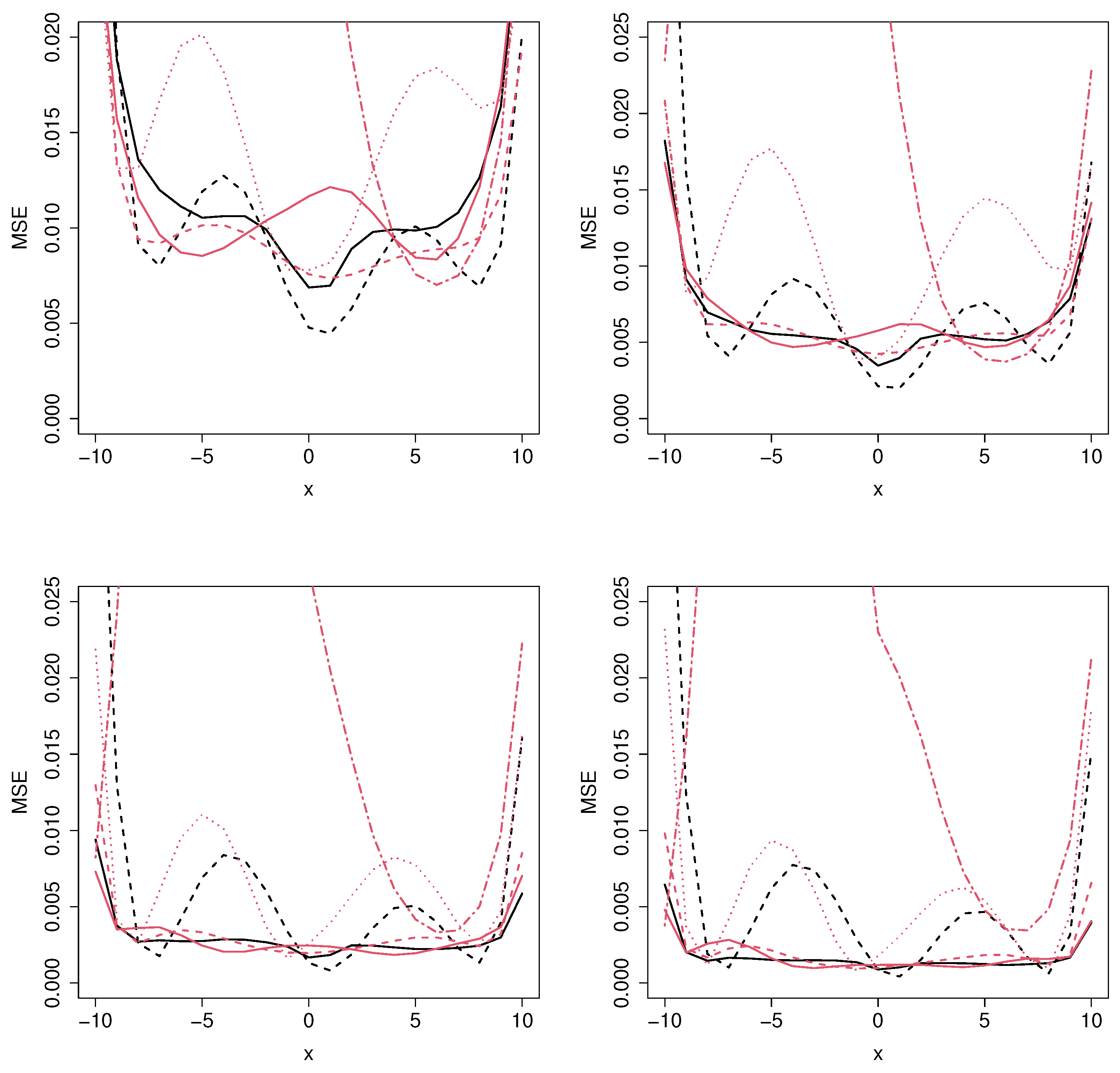
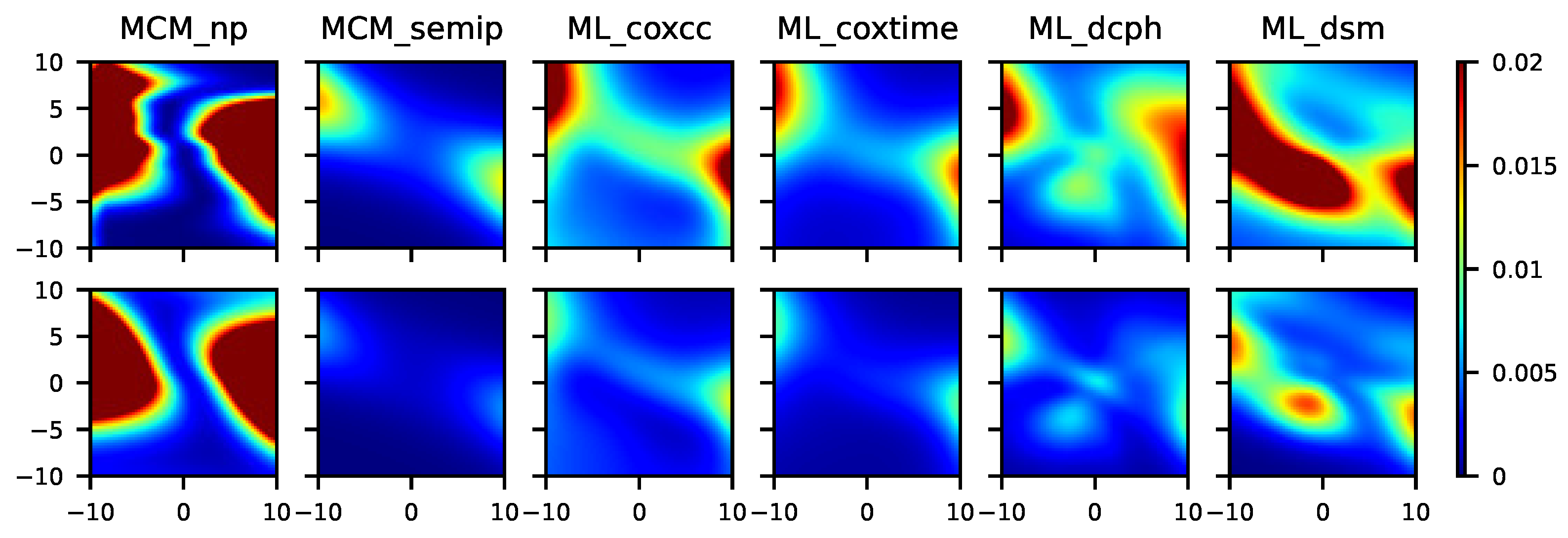
Note that, in Scenarios 1–4, the MSE in Equation (5) will be represented for a grid of covariate values. However, since in Scenarios 5–8 there are two covariates which influence the cure rate, the MSE is represented in a contour plot. The results related to Scenarios 1–8 are shown in Figure 2, Figure 3, Figure 4, Figure 5, Figure 6, Figure 7, Figure 8 and Figure 9, respectively.
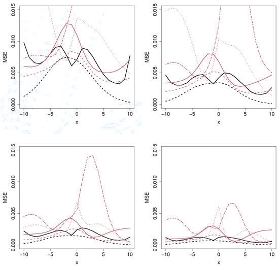
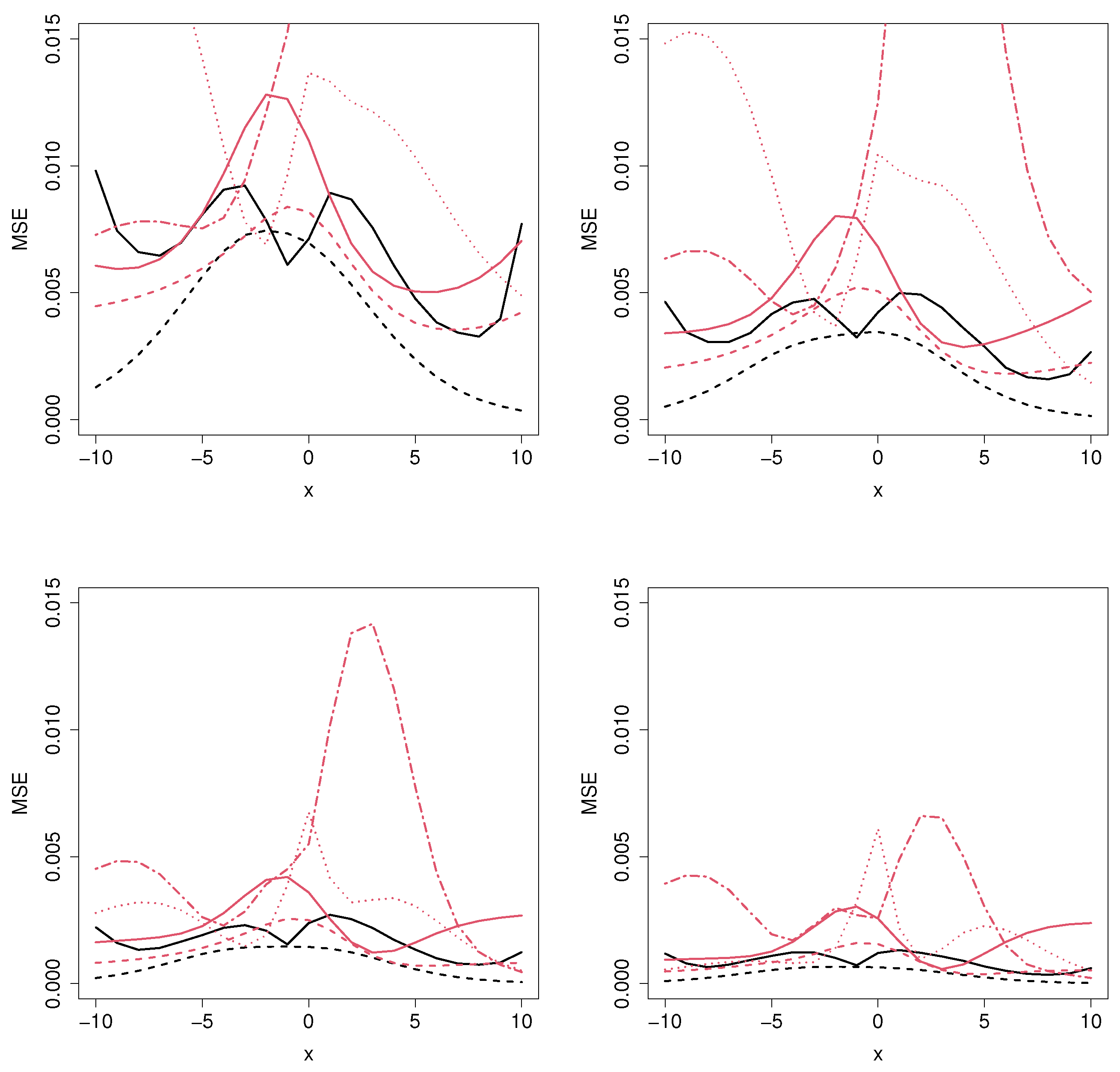
Figure 2.
Mean squared error for the MCM_np (black solid line), MCM_semip (black dashed line), ML_coxcc (red solid line), ML_coxtime (red dashed line), ML_dcph (red dotted line), and ML_dsm (red dot-dashed line), with sample sizes (top left), (top right), (bottom left), and (bottom right) for Scenario 1.
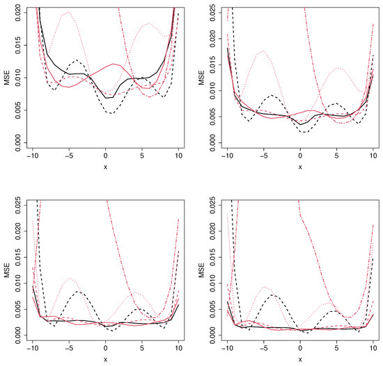
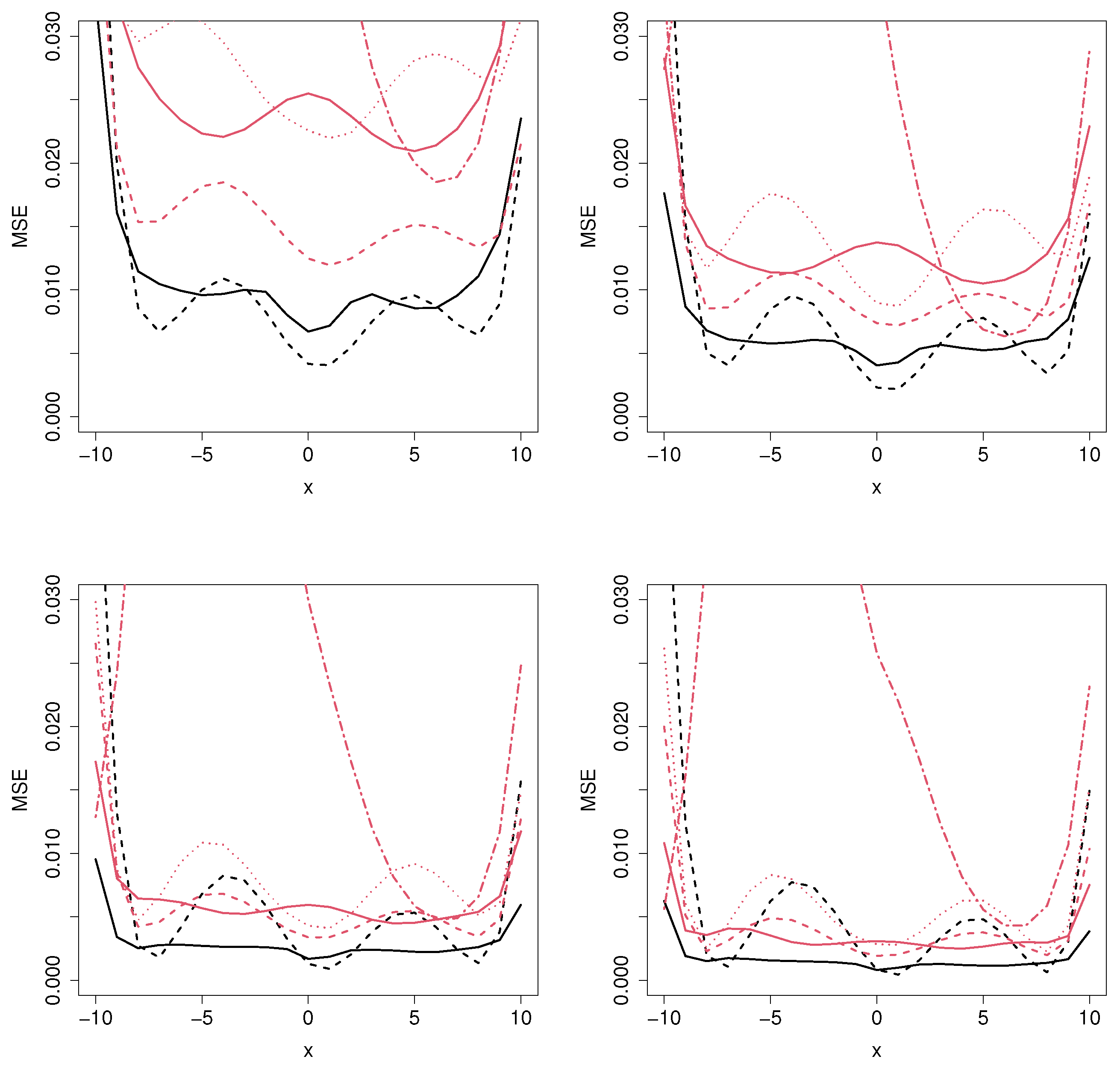
Figure 3.
Mean squared error for the MCM_np (black solid line), MCM_semip (black dashed line), ML_coxcc (red solid line), ML_coxtime (red dashed line), ML_dcph (red dotted line), and ML_dsm (red dot-dashed line), with sample sizes (top left), (top right), (bottom left), and (bottom right) for Scenario 2.
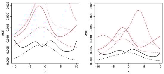
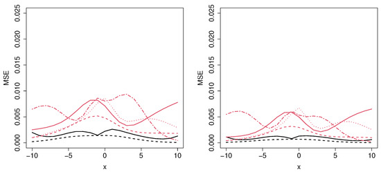
Figure 4.
Mean squared error for the MCM_np (black solid line), MCM_semip (black dashed line), ML_coxcc (red solid line), ML_coxtime (red dashed line), ML_dcph (red dotted line), and ML_dsm (red dot-dashed line), with sample sizes (top left), (top right), (bottom left), and (bottom right) for Scenario 3.
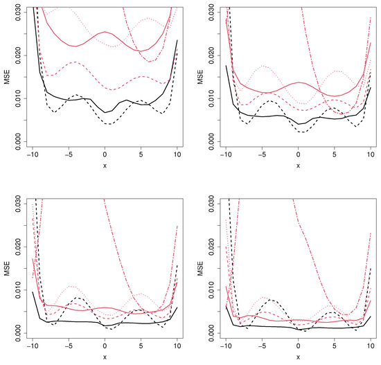
Figure 5.
Mean squared error for the MCM_np (black solid line), MCM_semip (black dashed line), ML_coxcc (red solid line), ML_coxtime (red dashed line), ML_dcph (red dotted line), and ML_dsm (red dot-dashed line), with sample sizes (top left), (top right), (bottom left), and (bottom right) for Scenario 4.
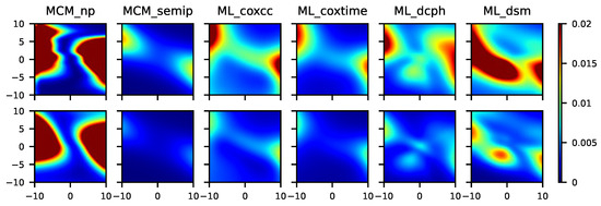
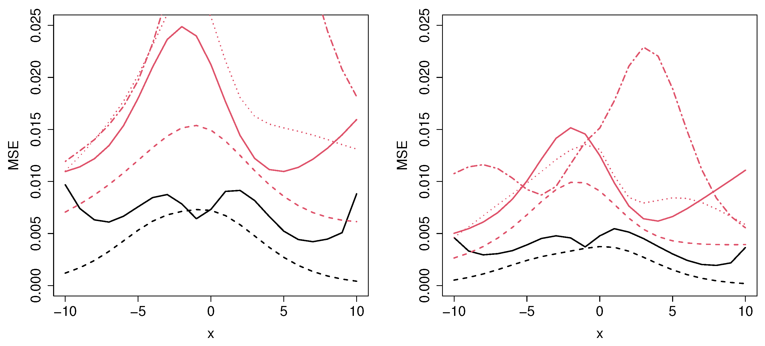
Figure 6.
From left to right, mean squared error for the MCM_np, MCM_semip, ML_coxcc, ML_coxtime, ML_dcph, and ML_dsm, with sample sizes (top) and (bottom) for Scenario 5.
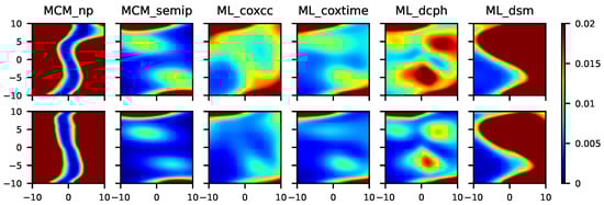
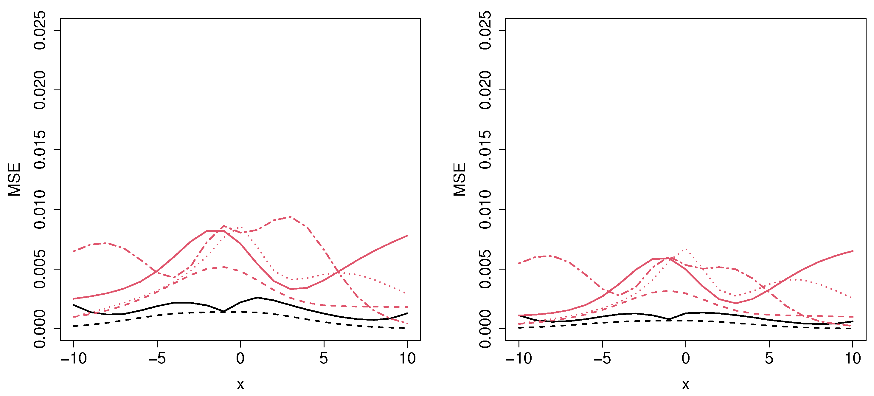
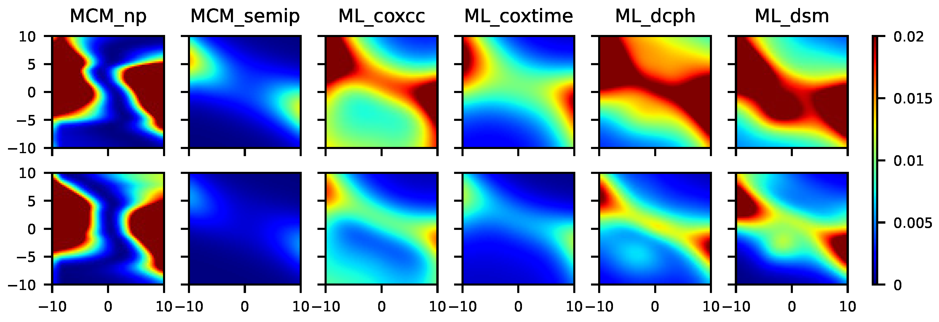
Figure 7.
From left to right, mean squared error for the MCM_np, MCM_semip, ML_coxcc, ML_coxtime, ML_dcph, and ML_dsm, with sample sizes (top) and (bottom) for Scenario 6.

Figure 8.
From left to right, mean squared error for the MCM_np, MCM_semip, ML_coxcc, ML_coxtime, ML_dcph, and ML_dsm, with sample sizes (top) and (bottom) for Scenario 7.
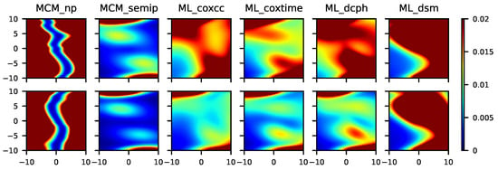
Figure 9.
From left to right, mean squared error for the MCM_np, MCM_semip, ML_coxcc, ML_coxtime, ML_dcph, and ML_dsm, with sample sizes (top) and (bottom) for Scenario 8.
As expected, as the sample size increases, the MSE decreases, proving the consistency of the methods. Figure 2 shows the results related to Scenario 1, where the underlying covariate effects can be well approximated by a logistic function. Therefore, the performance of the MCM_semip estimator is very good for all the sample sizes and for most of the covariate values. Regarding the MCM_np estimator, it is clear that, in this unfavorable context, it will lead to large MSE values. Not surprisingly, the second best method is the ML_coxtime, since the non-proportional hazard approach gives more flexibility for these scenarios.
The results obtained in Scenario 2 (see Figure 3), where there are no parametric or semiparametric assumptions, show the gain of using a nonparametric estimator. For moderate or large sample sizes and for most of the covariate values, the MCM_np outperforms the MCM_semip approach. However, the MCM_semip and the ML_coxcc are very competitive for small sample sizes, even beating the nonparametric methodology for a specific range of covariate values. Furthermore, it is important to note that the performance of the ML_coxtime approach is very similar to the one by the MCM_np method.
Regarding Figure 4 and Figure 5, which correspond to Scenarios 3 and 4, respectively, the MCM approaches outperform the ML methods for all the sample sizes and for most covariate values, as expected. The reason is that, in these scenarios, there are two covariates involved: one related to the cure rate and another one to the latency. However, since the ML methods cannot distinguish between those variables, the MSE error is not constant along the latency-involved variable, causing these models to be non-competitive in these situations.
In Figure 6, we can appreciate the difference regarding the MSE obtained in a semiparametric and in a nonparametric context. Note that, although the data were generated under a nonparametric model, the MCM_np is not expected to have a good performance since it does not account for multiple covariates in the cure rate. Specifically, the results related to the MCM_np approach show that, as the sample size increases, the MSE decreases very slowly, in some cases even negligibly. In Scenario 6 (see Figure 7), the minimum MSE is obtained with the MCM_semip, the ML_coxcc, and the ML_coxtime methods for the two considered sample sizes. As we observed in Scenarios 2 and 4, these semiparametric approaches are competitive even in nonparametric contexts.
Figure 8 shows the results related to a semiparametric context in which three different covariates are involved. As expected, the MCM_semip, ML_coxcc, and ML_coxtime approaches, due to their semiparametric nature, lead to small MSEs. Note that Scenario 8 (see Figure 9) is a non-favorable context for all of the methods. However, the performance of the MCM_semip is very good, beating the other methods. Again, the existence of a covariate only affecting the latency causes a bad performance of the ML methods.
5. Real Data Application
5.1. Application to COVID-19 Patients
The MCM and ML methods were applied to a dataset related to 8623 individuals who tested positive for COVID-19 infection in Galicia (Spain) during the first weeks of the pandemic (from 6 March 2020 until 7 May 2020). The data were provided by the Galician Public Health System. The event of interest is the hospital admission. Specifically, the variable of interest is the follow-up time, in days, since the individual tested positive for the first time until hospital admission. In this case, the term cured refers to individuals who did not need hospitalization. Since not all the infected subjects will suffer the event of interest, it is clear that a standard survival analysis is not appropriate and a cure model approach should be used.
Two covariates are considered: sex and age (from 0 to 106 years). The percentage of censoring is around 90%, depending on the sex. Table 2 shows a summary of the dataset.
Table 2.
Summary of the COVID-19 dataset.
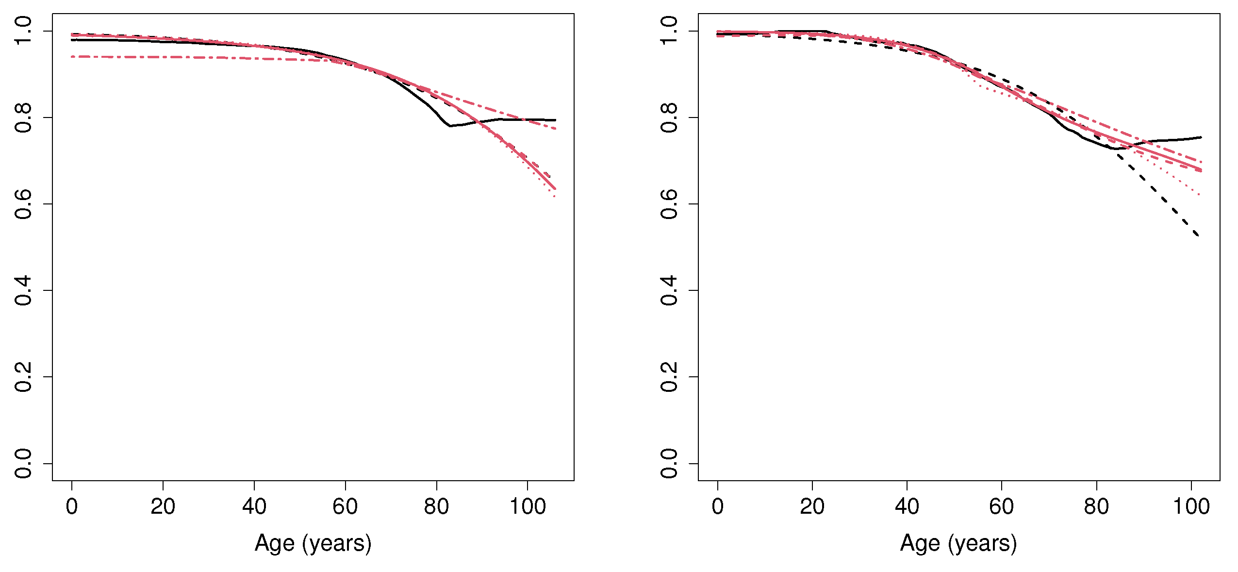
The cure rate estimation computed considering all the MCM and the ML approaches is shown in Figure 10. Regarding the MCM_np estimator, for both male and female patients aged below 50, the probability of not needing hospitalization is very close to 1. However, for individuals aged between 50 and 80, this probability decreases as the age increases. In addition, for patients above 80, the cure rate seems to become stabilized. Specifically, for female individuals above 80, the probability of not needing hospitalization is around 0.82, whereas for male subjects, this probability is around 0.77. The results obtained by the MCM_semip estimator and all the ML approaches deserve some comments. Note that these methods are not able to account for the, apparently, nonparametric underlying form of the data. In particular, although all the approaches lead to similar results for patients younger than 80, the MCM_semip estimation does not account for the constant cure rate related to patients above 80.
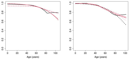
Figure 10.
Cure rate estimation for female (left) and male (right) patients, computed with MCM_np (black solid line), MCM_semip (black dashed line), ML_coxcc (red solid line), ML_coxtime (red dashed line), ML_dcph (red dotted line), and ML_dsm (red dot-dashed line) for the COVID-19 data set.
5.2. Application to Bone Marrow Transplant Patients
We consider the well-known dataset related to 137 bone marrow transplant patients (see [27,28]). The event of interest is the relapse of the disease, and the variable of interest is the disease-free survival time. Similarly as for the COVID-19 data application in Section 5.1, we considered two covariates: sex and age. The age varies from 8 to 45 years. A summary of the dataset is shown in Table 3.
Table 3.
Summary of the bmt dataset.
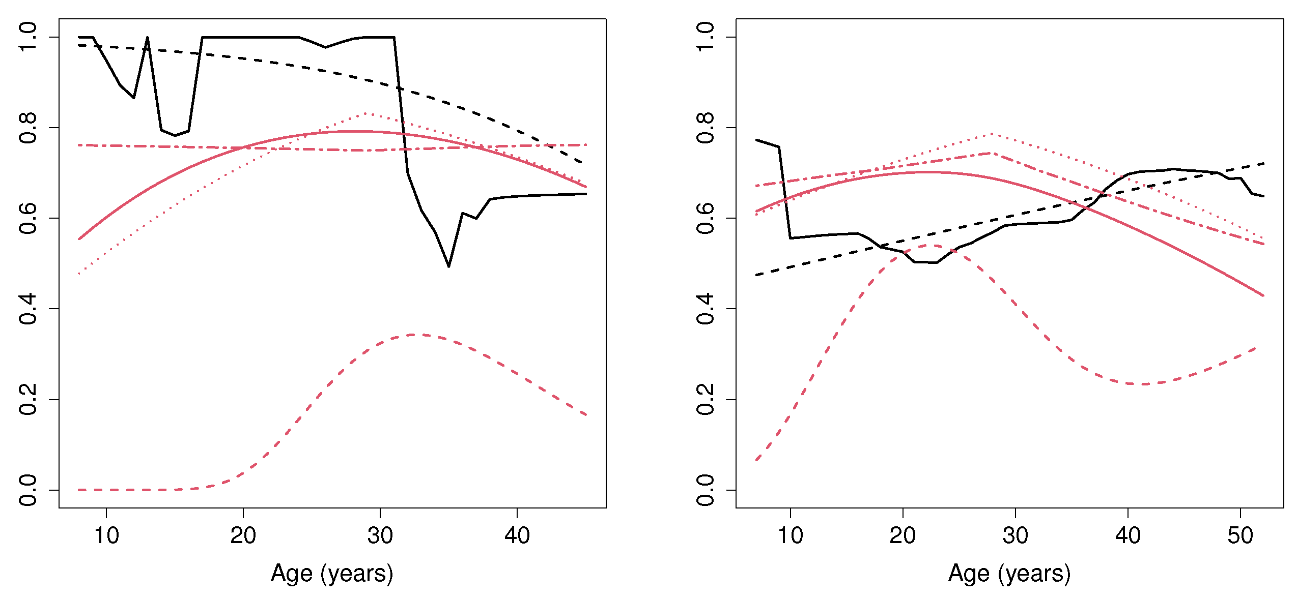
Figure 11 shows the estimated probability of cure (i.e., not suffering a relapse of the disease). Regarding MCM, we can observe that, for young female patients (aged below 30), this probability is between 0.8 and 1. However, for female patients above 30, the cure rate estimated with the MCM_np method considerably decreases and remains, approximately, constant at 0.6. Note that the methods defined under a semiparametric assumption (MCM_semip, ML_coxcc and ML_coxtime) are not able to detect this feature. It is important to mention that the MCM_np method considers the optimal bootstrap bandwidth required in the nonparametric estimator. If a larger bandwidth was considered, it would lead to a smoother cure rate estimation, especially for ages below 20, where the number of patients is not large. With respect to male subjects, it seems that the age does not influence the cure rate, since the estimated probability is around 0.6 and 0.8 for all ages. Furthermore, it is important to mention the results obtained by the ML_coxtime method, which differ considerably from all the other results. The reduced number of patients together with the underlying nonparametric curve may cause the ML_coxtime approach not to converge during the training procedure.
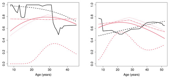
Figure 11.
Cure rate estimation for female (left) and male (right) patients, computed with MCM_np (black solid line), MCM_semip (black dashed line), ML_coxcc (red solid line), ML_coxtime (red dashed line), ML_dcph (red dotted line), and ML_dsm (red dot-dashed line) for the bone marrow transplant dataset.
6. Discussion
The outcome of this study shows that although machine learning approaches are powerful tools to deal with censored data, they have trouble fitting the real distribution. As far as we know, it is a relevant question that was not previously answered, since using the concordance index as metric does not provide information about how well the models adjust to the probability distribution.
In addition to that, our studies can offer some observations regarding the tested algorithms:
- There is a high discrepancy between the results obtained by the tested methods in recent classic survival analysis studies [7,9] and the ones obtained here, when cure is a possibility. Previous studies conclude that techniques like Random Survival Forests, DeepHit, and Deep Survival Machine achieve the best results in terms of the concordance index. However, when dealing with survival scenarios where cure is a possibility, the previous results do not translate. The experiments conducted in this paper conclude that mixture cure models and deep learning Cox-based approaches are the ones that best approximate the cure rate distribution.
- The MCM_semip approach is the best choice whenever the underlying cure rate function follows a semiparametric model. However, this is a hard assumption that is difficult to reassure when dealing with real case scenarios.
- Although it is never the best choice, the MCM_np approach obtains close-to-best results. Unfortunately, due to the curse of dimensionality, its implementation is only available for single-covariate contexts.
- The ML_coxtime algorithm is very accurate when dealing with both semiparametric and nonparametric cure rate functions.
- Both ML_coxcc and ML_dcph achieve similar results, proving to be a good choice whenever the cure rate function is not known.
- The ML_coxtime approach has to be treated carefully, as its solution can be unstable if a wrong neural network architecture is selected. Our experiments suggest that small networks (less than three hidden layers) tend to achieve more consistent results.
- With independence of the selected Deep Survival algorithm, the performance is highly affected in cases where the uncure rate and the latency are influenced by different covariates. In these cases, the MCM_semip achieves the best results, even when dealing with nonparametric scenarios.
Regarding the real data applications, some important remarks can also be made:
- ML_coxtime estimation in the application to bone narrow transplant is clearly far from the solutions provided by the other methods. We advise not to use it when the number of study samples is low.
- In addition, we do not recommend to use the ML_dhcp algorithm when the sample size is small. Figure 11, left, suggests the algorithm is not able to adjust to the cure rate estimation, providing a completely flat curve.
- The MCM_np is the only algorithm that is able to capture subtle changes in the cure rate estimation. Both machine learning Cox models and the MCM_semip method assume some conditions that cause a high degree of rigidity in their output. Therefore, in order to avoid biased estimations, we recommend the use of MCM_np when the underlying covariate effects cannot be well approximated by any parametric or semiparametric model.
7. Conclusions
In this work, we adapted ML methods used for classical survival analysis to estimate the probability of cure. Furthermore, we compared the performance of the introduced approaches. Two main groups have been evaluated: cure models (semiparametric and nonparametric approaches) and ML algorithms (mainly focused on deep learning solutions). An extensive simulation study was conducted, where the reliability of the evaluated methods was tested by measuring how they can estimate the cure probability. The results stipulate that MCM_np is the best choice, since it is the method which leads to the lowest MSE in each scenario. For contexts with multiple covariates, both MCM_semip and ML_coxtime are solid choices. In terms of reliability, we advise carefully using either ML_dsm and other ML approaches that were not included in the study, like DeepHit. Their output is highly influenced by either the model initialization or their hyper-parameters, making their output very unstable. For illustrative purposes, the methodologies were applied to two medical datasets, where the gain of using the nonparametric mixture cure model approach, which does not require any parametric or semiparametric assumptions to be fulfilled, was shown. In addition, it was observed how a small sample size affects the reliability of some machine learning methods, specifically, the ML_coxtime method.
Regarding future research lines, we propose to extend this work to evaluate the performance of these methods over the survival function, instead of only taking into account the survival rate. Additionally, we aim to define a fully nonparametric deep learning approach that can cope with some of the problems detected in the deep learning methods: discretization of the cure rate (DeepHit) and the rigidity of the Cox restrictions. In addition, a comparison of the latency estimation for the different methods will be of interest.
Author Contributions
Conceptualization, B.C. and A.L.-C.; Methodology, B.C. and A.L.-C.; Software, A.E.; Validation, A.E., B.C. and A.L.-C.; Formal Analysis, A.E., B.C. and A.L.-C.; Investigation, A.E., B.C. and A.L.-C.; Writing—Original Draft Preparation, A.E.; Writing—Review & Editing, B.C. and A.L.-C.; Visualization, A.E., B.C. and A.L.-C.; Supervision, B.C. and A.L.-C.; Project Administration, B.C. and A.L.-C.; Funding Acquisition, B.C. and A.L.-C. All authors have read and agreed to the published version of the manuscript.
Funding
This project was funded by the Xunta de Galicia (Axencia Galega de Innovación) Research projects COVID-19 presented in ISCIII IN845D 2020/26, Operational Program FEDER Galicia 2014–2020; by the Centro de Investigación de Galicia “CITIC”, funded by Xunta de Galicia and the European Union European Regional Development Fund (ERDF)-Galicia 2014–2020 Program, by grant ED431G 2019/01; and by the Spanish Ministerio de Economía y Competitividad (research projects PID2019-109238GB-C22 and PID2021-128045OA-I00). ALC was sponsored by the BEATRIZ GALINDO JUNIOR Spanish Grant from MICINN (Ministerio de Ciencia e Innovación) with code BGP18/00154. ALC was partially supported by the MICINN Grant PID2020-113578RB-I00 and partial support of Xunta de Galicia (Grupos de Referencia Competitiva ED431C-2020-14).
Institutional Review Board Statement
Not applicable.
Informed Consent Statement
Not applicable.
Data Availability Statement
The data related to Section 5.1 are available on request from the corresponding author. The data presented in Section 5.2 have been published in [28].
Acknowledgments
We gratefully acknowledge the support of NVIDIA Corporation with the donation of the Titan Xp GPU used for this research.
Conflicts of Interest
The authors declare no conflict of interest.
Abbreviations
The following abbreviations are used in this manuscript:
| AFT | Accelerated Failure Time |
| ANN | Artificial Neural Netowrks |
| ARD | Automatic Relevance Determination |
| IPCW | Inverse Probability of Censoring Weighting |
| MCM | Mixture Cure Models |
| ML | Machine Learning |
| MSE | Mean Squared Error |
| NB | Naive-Bayes |
| NMCM | Non-Mixture Cure Models |
| PH | Proportional Hazard |
| SVM | Support Vector Machine |
| SVR | Support Vector Regression |
References
- Leung, K.; Elashoff, R.M.; Afifi, A.A. Censoring issues in Survival Analysis. Annu. Rev. Public Health 1997, 18, 83–104. [Google Scholar] [CrossRef] [PubMed]
- Marubini, E.; Valsecchi, M. Analysing Survival Data from Clinical Trials and Observational Studies; John Wiley & Sons: Chichester, UK, 2004; Volume 15. [Google Scholar]
- Amico, M.; Van Keilegom, I. Cure models in survival analysis. Ann. Rev. Stat. Appl. 2018, 5, 311–342. [Google Scholar] [CrossRef]
- Pedrosa-Laza, M.; López-Cheda, A.; Cao, R. Cure models to estimate time until hospitalization due to COVID-19. Appl. Intell. 2022, 52, 794–807. [Google Scholar] [CrossRef] [PubMed]
- Peng, Y.; Yu, B. Cure Models. Methods, Applications, and Implementation; Chapman and Hall/CRC Press: Boca Raton, FL, USA, 2021. [Google Scholar]
- Steele, A.J.; Denaxas, S.C.; Shah, A.D.; Hemingway, H.; Luscombe, N.M. Machine learning models in electronic health records can outperform conventional survival models for predicting patient mortality in coronary artery disease. PLoS ONE 2018, 13, e0202344. [Google Scholar] [CrossRef]
- Kvamme, H.; Borgan, Ø.; Scheel, I. Time-to-Event Prediction with Neural Networks and Cox Regression. J. Mach. Learn Res. 2019, 20, 1–30. [Google Scholar]
- Spooner, A.; Chen, E.; Sowmya, A.; Sachdev, P.; Kochan, N.A.; Trollor, J.; Brodaty, H. A comparison of machine learning methods for survival analysis of high-dimensional clinical data for dementia prediction. Sci. Rep. 2020, 10, 20410. [Google Scholar] [CrossRef]
- Nagpal, C.; Li, X.; Dubrawski, A. Deep survival machines: Fully parametric survival regression and representation learning for censored data with competing risks. IEEE J. Biomed Health Inform. 2021, 25, 3163–3175. [Google Scholar] [CrossRef]
- Jiang, C.; Wang, Z.; Zhao, H. A prediction-driven mixture cure model and its application in credit scoring. Eur. J. Oper. Res. 2019, 277, 20–31. [Google Scholar] [CrossRef]
- Li, P.; Peng, Y.; Jiang, P.; Dong, Q. A support vector machine based semiparametric mixture cure model. Comput. Stat. 2020, 35, 931–945. [Google Scholar] [CrossRef]
- Štěpánek, L.; Habarta, F.; Malá, I.; Štěpánek, L.; Nakládalová, M.; Boriková, A.; Marek, L. Machine Learning at the Service of Survival Analysis: Predictions Using Time-to-Event Decomposition and Classification Applied to a Decrease of Blood Antibodies against COVID-19. Mathematics 2023, 11, 819. [Google Scholar] [CrossRef]
- Xu, J.; Peng, Y. Nonparametric cure rate estimation with covariates. Can. J. Stat. 2014, 42, 1–17. [Google Scholar] [CrossRef]
- Haybittle, J. The estimation of the proportion of patients cured after treatment for cancer of the breast. Brit. J. Radiol. 1959, 32, 725–733. [Google Scholar] [CrossRef] [PubMed]
- Haybittle, J. A two-parameter model for the survival curve of treated cancer patients. J. Am. Stat. Assoc. 1965, 60, 16–26. [Google Scholar] [CrossRef]
- Tsodikov, A.D.; Yakovlev, A.Y.; Asselain, B. Stochastic Models of Tumor Latency and Their Biostatistical Applications; World Scientific: Singapore, 1996; Volume 1. [Google Scholar]
- Yakovlev, A.Y.; Cantor, A.B.; Shuster, J.J. Parametric versus non-parametric methods for estimating cure rates based on censored survival data. Stat. Med. 1994, 13, 983–986. [Google Scholar] [CrossRef] [PubMed]
- Chen, M.H.; Ibrahim, J.; Sinha, D. A new Bayesian model for survival data with a surviving fraction. J. Am. Stat. Assoc. 1999, 94, 909–919. [Google Scholar] [CrossRef]
- Chen, K.; Jin, Z.; Ying, Z. Semiparametric analysis of transformation models with censored data. Biometrika 2002, 89, 659–668. [Google Scholar] [CrossRef]
- Tsodikov, A. A proportional hazards model taking account of long-term survivors. Biometrics 1998, 48, 1508–1516. [Google Scholar] [CrossRef]
- Tsodikov, A. Semiparametric models: A generalized self-consistency approach. J. R. Stat. Soc. Series B Stat. Methodol. 2003, 65, 759–774. [Google Scholar] [CrossRef]
- Zeng, D.; Yin, G.; Ibrahim, J.G. Semiparametric transformation models for survival data with a cure fraction. J. Am. Stat. Assoc. 2006, 101, 670–684. [Google Scholar] [CrossRef]
- Liu, X.; Xiang, L. Generalized accelerated hazards mixture cure models with interval-censored data. Comput. Stat. Data Anal. 2021, 161, 107248. [Google Scholar] [CrossRef]
- Tsodikov, A. Estimation of survival based on proportional hazards when cure is a possibility. Math. Comput. Model. 2001, 33, 1227–1236. [Google Scholar] [CrossRef]
- Kaplan, E.L.; Meier, P. Nonparametric Estimation from Incomplete Observations. J. Am. Stat. Assoc. 1958, 53, 457–481. [Google Scholar] [CrossRef]
- Beran, R. Nonparametric Regression with Randomly Survival Data; University of California: Berkeley, CA, USA, 1981. [Google Scholar]
- Klein, J.P.; Moeschberger, M.L. Survival Analysis: Techniques for Censored and Truncated Data; Springer: New York, NY, USA, 1997; Volume 1. [Google Scholar]
- Klein, J.P.; Moeschberger, M.L.; Yan, J. KMsurv: Data Sets from Klein and Moeschberger (1997), Survival Analysis; R package version 0.1-5; 2012. Available online: https://CRAN.R-project.org/package=KMsurv (accessed on 4 September 2023).
- López-Cheda, A.; Cao, R.; Jácome, M.A.; Van Keilegom, I. Nonparametric incidence estimation and bootstrap bandwidth selection in mixture cure models. Comput. Stat. Data Anal. 2017, 105, 144–165. [Google Scholar] [CrossRef]
- Boag, J.W. Maximum likelihood estimates of the proportion of patients cured by cancer therapy. J. R. Stat. Soc. Series B Stat. Methodol. 1949, 11, 15–53. [Google Scholar] [CrossRef]
- Berkson, J.; Gage, R.P. Survival curve for cancer patients following treatment. J. Am. Stat. Assoc. 1952, 47, 501–515. [Google Scholar] [CrossRef]
- Farewell, V.T. The use of mixture models for the analysis of survival data with long-term survivors. Biometrics 1982, 38, 1041–1046. [Google Scholar] [CrossRef] [PubMed]
- Yamaguchi, K. Accelerated failure-time regression models with a regression model of surviving fraction: An application to the analysis of “permanent employment” in Japan. J. Am. Stat. Assoc. 1992, 87, 284–292. [Google Scholar]
- Peng, Y.; Dear, K.B.; Denham, J. A generalized F mixture model for cure rate estimation. Stat. Med. 1998, 17, 813–830. [Google Scholar] [CrossRef]
- Denham, J.; Denham, E.; Dear, K.; Hudson, G. The follicular non-Hodgkin’s Lymphomas—I. The possibility of cure. Eur. J. Cancer 1996, 32, 470–479. [Google Scholar] [CrossRef]
- Wileyto, E.P.; Li, Y.; Chen, J.; Heitjan, D.F. Assessing the fit of parametric cure models. Biostatistics 2012, 14, 340–350. [Google Scholar] [CrossRef]
- de Oliveira, R.P.; de Oliveira Peres, M.V.; Martinez, E.Z.; Alberto Achcar, J. A new cure rate regression framework for bivariate data based on the Chen distribution. Stat. Methods Med. Res. 2022, 31, 2442–2455. [Google Scholar] [CrossRef] [PubMed]
- Müller, U.; Van Keilegom, I. Goodness-of-fit tests for the cure rate in a mixture cure model. Biometrika 2019, 106, 211–227. [Google Scholar] [CrossRef]
- Scolas, S.; El Ghouch, A.; Legrand, C.; Oulhaj, A. Variable selection in a flexible parametric mixture cure model with interval-censored data. Stat. Med. 2016, 35, 1210–1225. [Google Scholar] [CrossRef] [PubMed]
- Geng, Z.; Li, J.; Niu, Y.; Wang, X. Goodness-of-fit test for a parametric mixture cure model with partly interval-censored data. Stat. Med. 2022, 42, 407–421. [Google Scholar] [CrossRef]
- Musta, E.; Patilea, V.; Van Keilegom, I. A presmoothing approach for estimation in the semiparametric Cox mixture cure model. Bernoulli 2022, 28, 2689–2715. [Google Scholar] [CrossRef]
- Li, C.; Taylor, J.M.G. A semi-parametric accelerated failure time cure model. Stat. Med. 2002, 21, 3235–3247. [Google Scholar] [CrossRef]
- Wang, Y.; Zhang, J.; Tang, Y. Semiparametric estimation for accelerated failure time mixture cure model allowing non-curable competing risk. Stat. Theory Relat. Fields 2020, 4, 97–108. [Google Scholar] [CrossRef]
- Wang, Y.; Wang, W.; Tang, Y. A Bayesian semiparametric accelerate failure time mixture cure model. Int. J. Biostat. 2022, 18, 473–485. [Google Scholar] [CrossRef]
- Peng, Y.; Dear, K. A nonparametric mixture model for cure rate estimation. Biometrics 2000, 56, 237–243. [Google Scholar] [CrossRef]
- Lam, K.F.; Fong, D.Y.T.; Tang, O.Y. Estimating the proportion of cured patients in a censored sample. Stat. Med. 2005, 24, 1865–1879. [Google Scholar] [CrossRef]
- Corbière, F.; Commenges, D.; Taylor, J.M.G.; Joly, P. A penalized likelihood approach for mixture cure models. Stat. Med. 2009, 28, 510–524. [Google Scholar] [CrossRef] [PubMed]
- Wang, L.; Du, P.; Liang, H. Two-component mixture cure rate model with spline estimated nonparametric components. Biometrics 2012, 68, 726–735. [Google Scholar] [CrossRef] [PubMed]
- Hu, T.; Xiang, L. Efficient estimation for semiparametric cure models with interval-censored data. J. Multivar. Anal. 2013, 121, 139–151. [Google Scholar] [CrossRef]
- Amico, M.; Van Keilegom, I.; Legrand, C. The single-index/Cox mixture cure model. Biometrics 2019, 75, 452–462. [Google Scholar] [CrossRef]
- Maller, R.A.; Zhou, S. Estimating the proportion of immunes in a censored sample. Biometrika 1992, 79, 731–739. [Google Scholar] [CrossRef]
- Laska, E.M.; Meisner, M.J. Nonparametric estimation and testing in a cure model. Biometrics 1992, 48, 1223–1234. [Google Scholar] [CrossRef]
- Dabrowska, D. Uniform consistency of the kernel conditional Kaplan-Meier estimate. Ann. Stat. 1989, 17, 1157–1167. [Google Scholar] [CrossRef]
- López-Cheda, A.; Jácome, M.A.; Cao, R. Nonparametric latency estimation for mixture cure models. Test 2017, 26, 353–376. [Google Scholar] [CrossRef]
- López-Cheda, A.; Jácome, M.A.; López-de-Ullibarri, I. npcure: An R Package for Nonparametric Inference in Mixture Cure Models. R J. 2021, 13, 21–41. [Google Scholar] [CrossRef]
- López-de-Ullibarri, I.; López-Cheda, A.; Jácome, M.A. Npcure: Nonparametric Estimation in Mixture Cure Models; R package version 0.1-5; 2020. Available online: https://CRAN.R-project.org/package=npcure (accessed on 4 September 2023).
- López-Cheda, A.; Jácome, M.A.; Van Keilegom, I.; Cao, R. Nonparametric covariate hypothesis tests for the cure rate in mixture cure models. Stat. Med. 2020, 39, 2291–2307. [Google Scholar] [CrossRef]
- Wang, P.; Li, Y.; Reddy, C.K. Machine learning for survival analysis: A Survey. ACM Comput. Surv. 2019, 51, 1–36. [Google Scholar] [CrossRef]
- Gordon, L.; Olshen, R.A. Tree-structured survival analysis. Cancer Treat. Rep. 1985, 69, 1065–1069. [Google Scholar] [PubMed]
- Davis, R.B.; Anderson, J.R. Exponential survival trees. Stat. Med. 1989, 8, 947–961. [Google Scholar] [CrossRef] [PubMed]
- Kwak, L.W.; Halpern, J.; Olshen, R.A.; Horning, S.J. Prognostic significance of actual dose intensity in diffuse large-cell lymphoma: Results of a tree-structured survival analysis. J. Clin. Oncol. 1990, 8, 963–977. [Google Scholar] [CrossRef] [PubMed]
- LeBlanc, M.; Crowley, J. Relative risk trees for censored survival data. Biometrics 1992, 48, 411–425. [Google Scholar] [CrossRef]
- Huang, X.; Soong, S.; McCarthy, W.; Urist, M.; Balch, C. Classification of localized melanoma by the exponential survival trees method. Cancer 1997, 79, 1122–1128. [Google Scholar] [CrossRef]
- Huang, X.; Chen, S.; Soong, S. Piecewise exponential survival trees with time-dependent covariates. Biometrics 1998, 54, 1420–1433. [Google Scholar] [CrossRef]
- Ciampi, A.; Thiffault, J.; Nakache, J.; Asselain, B. Stratification by stepwise regression, correspondence analysis and recursive partition: A comparison of three methods of analysis for survival data with covariates. Comput. Stat. Data Anal. 1986, 4, 185–204. [Google Scholar] [CrossRef]
- Ciampi, A.; Chang, C.; Hogg, S.; McKinney, S. Recursive Partition: A Versatile Method for Exploratory-Data Analysis in Biostatistics. In Biostatistics: Advances in Statistical Sciences Festschrift in Honor of Professor V.M. Joshi’s 70th Birthday Volume V; Springer: Dordrecht, The Netherlands, 1987; pp. 23–50. [Google Scholar]
- Segal, M.R. Regression trees for censored data. Biometrics 1988, 44, 35–47. [Google Scholar] [CrossRef]
- Ishwaran, H.; Kogalur, U.B.; Blackstone, E.H.; Lauer, M.S. Random Survival Forests. Ann. Appl. Stat. 2008, 2, 841–860. [Google Scholar] [CrossRef]
- Schmid, M.; Wright, M.; Ziegler, A. On the use of Harrell’s C for clinical risk prediction via random survival forests. Expert Syst. Appl. 2016, 63, 450–459. [Google Scholar] [CrossRef]
- Andrade, J.; Valencia, J. A Fuzzy Random Survival Forest for Predicting Lapses in Insurance Portfolios Containing Imprecise Data. Mathematics 2023, 11, 198. [Google Scholar] [CrossRef]
- Awad, M.; Khanna, R. Support vector regression. In Efficient Learning Machines; Apress: Berkeley, CA, USA, 2015; pp. 67–80. [Google Scholar]
- Smola, A.J.; Schölkopf, B. Learning with Kernels; Citeseer: New York, NY, USA, 1998; Volume 4. [Google Scholar]
- Har-Peled, S.; Roth, D.; Zimak, D. Constraint classification: A new approach to multiclass classification. In Proceedings of the International Conference on Algorithmic Learning Theory, Virtual, 16–19 March 2021; Springer: Heidelberg, Germany, 2002; pp. 365–379. [Google Scholar]
- Khan, F.M.; Zubek, V.B. Support vector regression for censored data (SVRc): A novel tool for survival analysis. In Proceedings of the 2008 Eighth IEEE International Conference on Data Mining, IEEE, Pisa, Italy, 15–19 December 2008; pp. 863–868. [Google Scholar]
- Van Belle, V.; Pelckmans, K.; Van Huffel, S.; Suykens, J.A. Support vector methods for survival analysis: A comparison between ranking and regression approaches. Artif. Intell. Med. 2011, 53, 107–118. [Google Scholar] [CrossRef] [PubMed]
- Kiaee, F.; Sheikhzadeh, H.; Mahabadi, S.E. Relevance vector machine for survival analysis. IEEE Trans. Neural. Netw. Learn. Syst. 2015, 27, 648–660. [Google Scholar] [CrossRef] [PubMed]
- Lisboa, P.J.; Wong, H.; Harris, P.; Swindell, R. A Bayesian neural network approach for modelling censored data with an application to prognosis after surgery for breast cancer. Artif. Intell. Med. 2003, 28, 1–25. [Google Scholar] [CrossRef]
- Fard, M.J.; Wang, P.; Chawla, S.; Reddy, C.K. A bayesian perspective on early stage event prediction in longitudinal data. IEEE Trans. Knowl. Data Eng. 2016, 28, 3126–3139. [Google Scholar] [CrossRef]
- Rosenblatt, F. The perceptron: A probabilistic model for information storage and organization in the brain. Psychol. Rev. 1958, 65, 386. [Google Scholar] [CrossRef]
- Liestbl, K.; Andersen, P.K.; Andersen, U. Survival analysis and neural nets. Stat. Med. 1994, 13, 1189–1200. [Google Scholar] [CrossRef]
- Mariani, L.; Coradini, D.; Biganzoli, E.; Boracchi, P.; Marubini, E.; Pilotti, S.; Salvadori, B.; Silvestrini, R.; Veronesi, U.; Zucali, R.; et al. Prognostic factors for metachronous contralateral breast cancer: A comparison of the linear Cox regression model and its artificial neural network extension. Breast Cancer Res. Treat. 1997, 44, 167–178. [Google Scholar] [CrossRef]
- Brown, S.F.; Branford, A.J.; Moran, W. On the use of artificial neural networks for the analysis of survival data. IEEE Trans. Neural. Netw. Learn. Syst. 1997, 8, 1071–1077. [Google Scholar] [CrossRef]
- Cox, D.R. Regression models and life-tables. J. R. Stat. Soc. Series B Stat. Methodol. 1972, 34, 187–202. [Google Scholar] [CrossRef]
- Cox, D.R. Partial likelihood. Biometrika 1975, 62, 269–276. [Google Scholar] [CrossRef]
- Faraggi, D.; Simon, R. A neural network model for survival data. Stat. Med. 1995, 14, 73–82. [Google Scholar] [CrossRef] [PubMed]
- Yousefi, S.; Amrollahi, F.; Amgad, M.; Dong, C.; Lewis, J.E.; Song, C.; Gutman, D.A.; Halani, S.H.; Vega, J.E.V.; Brat, D.J.; et al. Predicting clinical outcomes from large scale cancer genomic profiles with deep survival models. Sci. Rep. 2017, 7, 11707. [Google Scholar] [CrossRef] [PubMed]
- Luck, M.; Sylvain, T.; Cardinal, H.; Lodi, A.; Bengio, Y. Deep learning for patient-specific kidney graft survival analysis. arXiv 2017, arXiv:1705.10245. [Google Scholar]
- Katzman, J.L.; Shaham, U.; Cloninger, A.; Bates, J.; Jiang, T.; Kluger, Y. DeepSurv: Personalized treatment recommender system using a Cox proportional hazards deep neural network. BMC Med. Res. Methodol. 2018, 18, 1–12. [Google Scholar] [CrossRef]
- Ching, T.; Zhu, X.; Garmire, L.X. Cox-nnet: An artificial neural network method for prognosis prediction of high-throughput omics data. PLoS Comput. Biol. 2018, 14, e1006076. [Google Scholar] [CrossRef]
- Kvamme, H.; Borgan, Ø. Continuous and discrete-time survival prediction with neural networks. Lifetime Data Anal. 2021, 27, 710–736. [Google Scholar] [CrossRef]
- Beaulac, C.; Rosenthal, J.S.; Pei, Q.; Friedman, D.; Wolden, S.; Hodgson, D. An evaluation of machine learning techniques to predict the outcome of children treated for Hodgkin-Lymphoma on the AHOD0031 trial. Appl. Artif. Intell. 2020, 34, 1100–1114. [Google Scholar] [CrossRef]
- Srujana, B.; Verma, D.; Naqvi, S. Machine Learning vs. Survival Analysis Models: A study on right censored heart failure data. Commun. Stat. Simul. Comput. 2022, 0, 1–18. [Google Scholar] [CrossRef]
- Lee, C.; Zame, W.R.; Yoon, J.; Van der Schaar, M. Deephit: A deep learning approach to survival analysis with competing risks. In Proceedings of the Thirty-Second AAAI Conference on Artificial Intelligence, New Orleans, LA, USA, 2–7 February 2018. [Google Scholar]
- Gensheimer, M.F.; Narasimhan, B. A scalable discrete-time survival model for neural networks. PeerJ 2019, 7, e6257. [Google Scholar] [CrossRef] [PubMed]
- Xie, Y.; Yu, Z. Mixture cure rate models with neural network estimated nonparametric components. Comput. Stat. 2021, 36, 2467–2489. [Google Scholar] [CrossRef]
- Xie, Y.; Yu, Z. Promotion time cure rate model with a neural network estimated non-parametric component. Stat. Med. 2021, 40, 3516–3532. [Google Scholar] [CrossRef] [PubMed]
- Pal, S.; Aselisewine, W. A semiparametric promotion time cure model with support vector machine. Ann. Appl. Stat. 2023, 17, 2680–2699. [Google Scholar] [CrossRef]
- Kim, D.; Lee, S.; Kwon, S.; Nam, W.; Cha, I.; Kim, H. Deep learning-based survival prediction of oral cancer patients. Sci. Rep. 2019, 9, 6994. [Google Scholar] [CrossRef]
- Antosz, K.; Machado, J.; Mazurkiewicz, D.; Antonelli, D.; Soares, F. Systems Engineering: Availability and Reliability. Appl. Sci. 2022, 12, 2504. [Google Scholar] [CrossRef]
- Martyushev, N.; Malozyomov, B.; Sorokova, S.; Efremenkov, E.; Valuev, D.; Qi, M. Review Models and Methods for Determining and Predicting the Reliability of Technical Systems and Transport. Mathematics 2023, 11, 3317. [Google Scholar] [CrossRef]
- Antolini, L.; Boracchi, P.; Biganzoli, E. A time-dependent discrimination index for survival data. Stat. Med. 2005, 24, 3927–3944. [Google Scholar] [CrossRef]
- Kuk, A.; Chen, C. A mixture model combining logistic regression with proportional hazards regression. Biometrika 1992, 79, 531–541. [Google Scholar] [CrossRef]
- Nagpal, C.; Potosnak, W.; Dubrawski, A. Auton-survival: An open-source package for regression, counterfactual estimation, evaluation and phenotyping with censored time-to-event data. In Proceedings of the Machine Learning for Healthcare Conference, PMLR, Durham, NC, USA, 5–6 August 2022; pp. 585–608. [Google Scholar]


Disclaimer/Publisher’s Note: The statements, opinions and data contained in all publications are solely those of the individual author(s) and contributor(s) and not of MDPI and/or the editor(s). MDPI and/or the editor(s) disclaim responsibility for any injury to people or property resulting from any ideas, methods, instructions or products referred to in the content. |
© 2023 by the authors. Licensee MDPI, Basel, Switzerland. This article is an open access article distributed under the terms and conditions of the Creative Commons Attribution (CC BY) license (https://creativecommons.org/licenses/by/4.0/).