Article

Selecting and Weighting Mechanisms in Stock Portfolio Design Based on Clustering Algorithm and Price Movement Analysis

1
Department of Statistics, Faculty of Mathematics and Natural Sciences, Universitas Padjadjaran, Sumedang 45363, Indonesia
2
Department of Mathematics, Faculty of Mathematics and Natural Sciences, Universitas Padjadjaran, Sumedang 45363, Indonesia
3
Doctoral Program of Mathematics, Faculty of Mathematics and Natural Sciences, Universitas Padjadjaran, Sumedang 45363, Indonesia
4
Magister Program of Mathematics, Faculty of Mathematics and Natural Sciences, Universitas Padjadjaran, Sumedang 45363, Indonesia
*
Author to whom correspondence should be addressed.
Mathematics 2023, 11(19), 4151; https://doi.org/10.3390/math11194151
Submission received: 18 August 2023 / Revised: 26 September 2023 / Accepted: 28 September 2023 / Published: 2 October 2023
(This article belongs to the Special Issue Economic Model Analysis and Application)

Abstract

:
The fundamental stages in designing a stock portfolio are each stock’s selection and capital weighting. Selection and weighting must be conducted through diversification and price movement analysis to maximize profits and minimize losses. The problem is how the technical implementations of both are carried out. Based on this problem, this study aims to design these selection and weighting mechanisms. Stock selection is based on clusters and price movement trends. The optimal stock clusters are formed using the K-Means algorithm, and price movement analyses are carried out using the moving average indicator. The selected stocks are those whose prices have increasing trends with the most significant Sharpe ratio in each cluster. Then, the capital weighting for each preferred stock is carried out using the mean-variance model with transaction cost and income tax. After designing the mechanism, it is applied to Indonesia’s 80 index stock data. In addition, a comparison is conducted between the estimated portfolio return and the actual one day ahead. Finally, the sensitivity of investors’ courage in taking risks to their profits and losses is also analyzed. This research is expected to assist investors in diversification and price movement analysis of the stocks in the portfolios they form.

1. Introduction

One of the crucial stages in forming a stock investment portfolio is the selection of stocks [1,2]. The selection must be based on the characteristics of certain stocks, for example, the average profit and loss. In detail, the stocks selected must have different characteristics. This selection of stocks in a portfolio with different characteristics is referred to as diversification. Diversification can minimize portfolio losses [3,4]. In simple terms, if the portfolio contains stocks with the same characteristics, the loss experienced when the price of these falls is enormous. However, if diversification is applied, the loss of one stock can be covered by another stock whose price rises. In other words, diversification also makes the profit opportunities from the portfolio greater. In addition to considering the different characteristics, the selection of stocks in forming a portfolio must also consider price movements [5,6]. The selected stock must have a price movement that tends to rise. This is because stocks with an increasing price trend generally indicate high demand. If that happens, the stock price will too rise [7,8]. In other words, selecting stocks with rising price trends can increase opportunities for profits and reduce opportunities for losses that may occur in the future.
After the stock selection, another important step is the capital weighting for each stock in the portfolio [9,10]. This weighting can practically be conducted based on minimizing losses and maximizing profits, as first introduced by Markowitz [11]. In general, stocks with large average losses also have large average profits, and vice versa [12,13]. If investors want to avoid the risk of large losses, the capital weight on stocks with high average losses can be reduced. The consequence is that the return obtained is small. However, if investors are willing to take the risk of loss, the weight of stocks with large average losses can be increased. Thus, the opportunity for profit is also greater. It should be noted that the weight allocated to each stock should be positive. In other words, stocks are not bought on debt. It avoids the risk of default on debt when stocks fail [14,15,16,17]. Apart from minimizing losses and maximizing profits, investors must consider administrative costs, e.g., transaction costs and income taxes. Even though the value of both is small, both can be detrimental if the profit is small. This can give rise to a negative mean of portfolio return [18].
The development of studies examining the mechanism of weighting stock capital in forming investment portfolios is briefly explained in this paragraph. Markowitz [19] first introduced a capital weighting model in portfolios called mean-variance. Then, Sharpe [20] made the model into a matrix form to make it more efficient in computing time. These two pieces of study became the basis for future research, e.g., the capital asset pricing model (CAPM) [21] and the minimax portfolio model [22]. Then, Björk et al. [23] developed a mean-variance model in continuous time, where risk aversion is assumed to depend on investors’ wealth. Using the conic programming approach, Ghaoui et al. [24] developed the Markowitz model for worst-case value-at-risk. Then, Abdurakhman [25] introduced a robust portfolio mean-variance-skewness model to accommodate abnormal and asymmetric problems of stock returns. Then, Faramarzi et al. [26] introduced the equilibrium optimizer model for weighting stock capital in portfolios. Zhou and Li [27] designed a multiobjective optimization model that is stochastic, linear-quadratic (LQ), and has a continuous time index in the capital stock weighting problem. Zhu et al. [28] introduced particle swarm optimization (PSO) to solve the problem of optimizing multiobjective portfolio weights with non-linear constraints. Kalfin et al. [29] and Ryoo [30] introduced a mean-absolute-deviation model for the unique case weighting stock capital, where the covariance matrix between stock returns is singular. Wang and Gan [31] designed a weighting model for stock capital in a portfolio with targeted performance criteria through neurodynamic optimization. Dai and Kang [32] developed a mean-variance model by considering the L1 regulation of the objective function and the shrinkage method of Ledoit and Wolf [33] in forming the return covariance matrix. Then, Mba et al. [34] developed a mean-variance model using behavioral mean-variance (BMV) and copula behavioral mean-variance (CBMV). Du [35] presented a new mean-variance model built using a stationary portfolio of cointegrated stocks based on deep learning. Li et al. [36] developed a mean-variance model whose modal weight allocation is given by a predictive control model with the aim of risk parity.
Since the 2000s, the topic has focused on weighting stock capital and expanded to stock selection mechanisms through clustering. Chen and Huang [37] introduced a clustering-based stock selection mechanism through the K-Means algorithm with the following attributes: average return, the standard deviation of returns, the Treynor index, and turnover rate. Then, they weighted the capital using a fuzzy return rate through a mean-variance model. Sinha et al. [38] clustered the stocks in the portfolio using a genetic algorithm and weighted the capital using a minimized variance portfolio model. Golosnoy and Okhrin [39] developed a mean-variance model by involving shrinkage in measuring the mean of the covariance matrix of stock returns. Ren et al. [40] applied the K-Means algorithm to cluster stocks with attribute correlation coefficients between stocks. Fleischhacker et al. [41] clustered stock data in the energy sector using the K-Means algorithm with the attributes of heat demand, electricity demand, cooling demand, solar PV supply, and solar thermal collector supply. Then, they weighted the capital using Pareto optimization and two objectives: costs and carbon emissions. Tola et al. [42] clustered stock data using the average linkage algorithm with characteristic attributes of the correlation coefficient between stock returns and weighted the capital using a mean-variance model. Then, in their research, Chen et al. [43] and Cheong et al. [44] used the K-Means algorithm with the characteristic attribute mean of return for clustering stock data. Then, they weighted the capital using a mean-variance model. Musmeci et al. [45] compared the K-Medoids, linkage, and directed bubble hierarchical tree methods with the attributes of the correlation coefficient between stocks. Fawaid et al. [46] compared the K-Means and average linkage clustering algorithms with the mean of return and variance of return attributes. Then, they weighted the capital using the mean-value-at-risk model. Khan and Mehlawat [47] clustered stocks using fuzzy C-means clustering and weighted stock capital in the portfolio using a genetic algorithm. Finally, Hussain et al. [48] proposed new mechanisms for cluster stocks, which are the Adaptive Neuro-Fuzzy Inference System (ANFIS) and Induced Ordered Weighted Averaging (IOWA) model.
Several studies have also considered the price movement analysis in their selection and weighting of the capital of stocks in the portfolio. Navarro et al. [49] carried out stock clustering using K-Means, price analysis using the MACD method, and capital weighting using the mean-variance model. Aheer et al. [50] clustered stocks in a portfolio using a feed-forward neural network, analyzed their price movements using geometric Brownian motion, and weighted the capital using a mean-variance model. Then, Sukono et al. [51] analyzed the stock price movement using ARIMA-GARCH and weighted its capital using the mean-value-at-risk model. Then, Du and Tanaka-Ishii [52] analyzed stock price movement using a NEWS-STock space with Event Distribution (NESTED) and weighted the capital using a mean-variance model. Chang et al. [53] conducted mixed integer programming for weighting the capital in the portfolio. They took advantage of price movements using behavioral stock (B-stock). Varga-Haszonits and Kondor [54] investigated the capital weight of the stock in the portfolio using minimum variance portfolio optimization. The stock price movement was assumed to follow the constant conditional correlation GARCH process proposed by Bollerslev. Thuankhonrak et al. [55] carried out stock clustering using a support vector machine (SVM) and artificial neural network (ANN), price analysis using the ARIMA and Holt Winter method, and capital weighting using a mean-variance model.
Gaps from previous studies are discussed in this paragraph. In general, stock clustering in previous studies used K-Means. This is because the method is intuitive. Stock clusters are determined based on the similarity of their attributes. This similarity is seen from the closest distance between the stock attribute values and the center point of the cluster (called the centroid), e.g., Euclidean distance [40]. Then, the stocks selected are the stocks with the best characteristic attribute values in each cluster. Of course, the selected stocks have a positive average return. Then, in general, the capital weighting of stocks in the portfolio is carried out using the mean-variance model. However, no one has integrated the mean-variance model with transaction cost and income tax variables, even though transaction costs and income tax are essential to involve. Finally, analysis of stock price movements in previous studies was not focused on a specific method. In other words, the methods used vary. However, there has been no research using moving-average indicators. This method is simple and fast for practitioners in the capital market for short-term investments. Therefore, this gap is used as a novelty in this study.
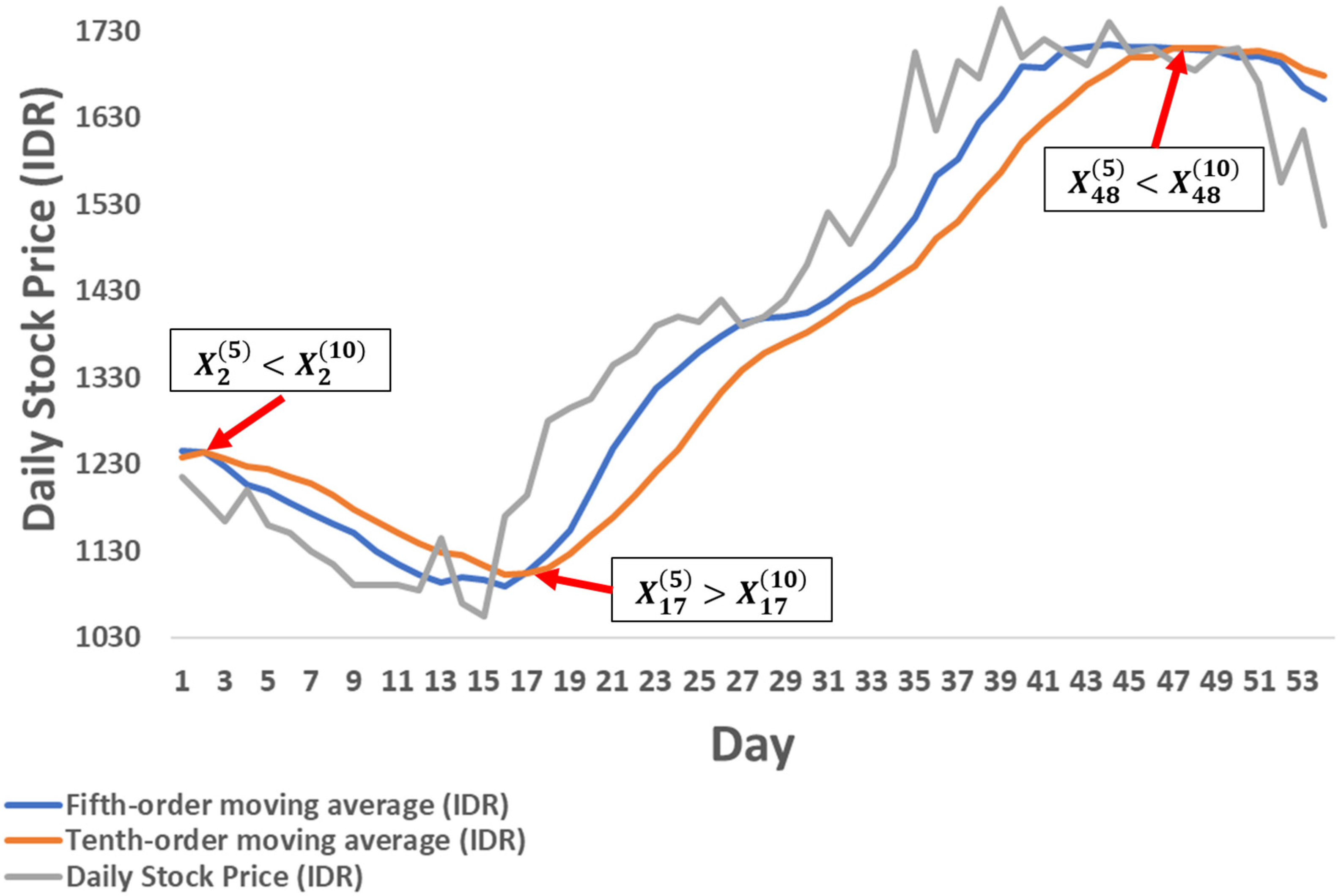
Based on this introduction, this study aims to develop a mechanism for selecting and weighing the capital of stocks in a portfolio based on a clustering algorithm and price movement analysis. Stocks with a positive mean of returns are selected for clustering. Clustering is conducted using the K-Means method based on the attributes of the mean and variance of returns. This method is intuitively based on the closest distance between stock attributes and the centroid of a cluster, as mentioned in the previous paragraph. After clustering is conducted, stocks with an increasing trend are considered to reselect again. The increasing trend in this research is explored weekly using the fifth and tenth orders of moving average values, abbreviated as MA5 and MA10. If MA5 exceeds MA10, daily stock prices this week tend to be higher than in the previous weeks. In other words, the stock has an increasing price tendency now. Therefore, the selected stocks must have an MA5 greater than MA10. After increasing trend reselection, the best stock from each cluster is chosen based on the Sharpe ratio measure. After that, the capital weight of each stock is determined using the mean-variance model with the addition of administrative costs, e.g., transaction costs and income taxes. The model is also intuitive, based on the investor’s goal of maximizing the return mean and minimizing the return variance. After the mechanism is designed, its application is conducted on Index 80 stock data in Indonesia. Finally, the sensitivity of investors’ risk aversion, transaction cost, income tax, and increasing trend to the mean and variance of return is analyzed. This research is expected to assist investors in selecting and weighing stocks in a portfolio designed based on cluster-based and price movement analysis.

2. Stock Selection and Weighting Framework

2.1. Stock Clustering with Two-Dimensional K-Means

Data clustering using the K-means algorithm is based on the closest distance to a particular centroid [56]. The K-means algorithm is carried out iteratively until there is no change between the new and old centroids [57,58]. In other words, the iteration stops when the members of each current cluster are equal to the members of each previous cluster. The cluster from the last iteration is the result. This method is suitable for clustering that uses not too many attributes [42,46,59]. Since this research uses two attributes, namely the mean and variance of stock returns, it is appropriate to use this method.
Suppose that the number of stocks is M , and the number of clusters is Q . Then, suppose that the distance between data and cluster centroids is measured using the Euclidean distance. The K-means clustering algorithm, in this case, is briefly given in Algorithm 1.
Algorithm 1. Two-Dimensional K-Means based on Euclidean Distance
Input am: the set of vectors of the mean and variance of returns from the m-th stock,
                                                   m = 1, 2, …, M
vq: the initial centroid for q-th cluster, q = 1, 2, …, Q
Output   v q : the latest centroid for q-th cluster, q = 1, 2, …, Q
k q : the latest q-th cluster, q = 1, 2, …, Q
Processes:
(1)
//Calculating the distance between the vector am and each centroid
for q in {1, 2, …, Q}
for m in {1, 2, …, M}
                                             dq,m= ‖amvq2
end
end
(2)
//Defining the empty vector set for each cluster
for q in {1, 2, …, Q}
kq = []
end
(3)
//Determining the members of each cluster
for m in {1, 2, …, M}
                                       p = min⁡{dq,m; q = 1, 2, …, Q}
if p = d1,m
                                             k1 = [k1,am]
else if p = d2,m
                                             k2 = [k2 am]
                                                         ⋮
else if p = dQ−1,m
                                             kQ−1 = [kQ−1 am]
else p = dQ,m
                                             kQ = [kQ am]
end
end
(4)
//Determining new centroids
for q in {1, 2, …, Q}
vq = average of kq
end
(5)
Repeat steps (1) through (4) until there is no difference between the new and previous centroids.

2.2. Selecting Stocks in Each Cluster with Indicators of Short-Term Price Increases

This study’s increasing trend of stock prices is analyzed using the fifth and tenth orders of moving average values, abbreviated as MA5 and MA10 [60,61]. The fifth order represents the number of working days in one week, while the tenth order represents the number of working days in two weeks. Intuitively, if MA5 is higher than MA10, the stock price has an increasing tendency [62] because daily stock prices this week tend to be higher than in the previous weeks. This intuition also applies to the opposite situation, where if MA5 is smaller than MA10, the stock price has a decreasing tendency [62] because daily stock prices this week tend to be smaller than in the previous week. Then, if MA5 is equal to M10, the stock price movement tendency cannot be concluded. The MA5 and MA10 are calculated, respectively using the following equation:
X   T + 1 5 = 1 5 t = 1 5 X T t + 1
and
X T + 1 10 = 1 10 t = 1 10 X T t + 1 ,
where X t represents the stock price on t working days before today. Mathematically, if X T + 1 5 > X T + 1 10 , the stock price has an increasing tendency now, whereas if X T + 1 5 < X T + 1 10 , the stock price has a decreasing tendency now. Then, if X T + 1 5 = X T + 1 10 , the result cannot be concluded [60]. It can be seen in Figure 1, where when X t 5 < X t 10 , the stock price at day t tends to decrease. Then, when X t 5 > X t 10 , the stock price at day t tends to increase.

2.3. Final Selection

Stocks with an increasing tendency in each cluster were reselected. Reselection is conducted using the value of the Sharpe ratio. The value of the Sharpe ratio r is determined using the following equation [63]:
r = m e a n   o f   r e t u r n s t a n d a r d   d e v i a t i o n   o f   r e t u r n .
Stocks with an increasing tendency and the highest Sharpe ratio value in each cluster are those chosen in the portfolio preparation [64]. As a small note, the mean in Equation (3) represents the mean of stock returns over the period considered, while the means in Equations (1) and (2), respectively, represent the mean of stock prices over the last five and ten working days.

2.4. Capital Weighting in Portfolios Using the Mean-Variance Model

Markowitz [19] introduced the mean-variance model in the problem of the capital weighting of stocks in an investment portfolio in single period time, e.g., daily and weekly. Intuitively, this model is based on investors’ tendency to maximize profits and minimize losses from the portfolio simultaneously when they invest their capital [65]. In the mean-variance model, the profit is represented by the mean of return, while the variance of return represents the loss.
Suppose that the total capital of the stock portfolio containing M stocks is W in currency units, and the capital weight of each stock in it is { w m , m = 1 ,   2 , , M } . To facilitate modeling, the value of W is set to 1. Then, suppose that the return of each stock in each portfolio is expressed as a normal random variable R m , m = 1 ,   2 ,   , M with mean μ m and variance σ m 2 . The state of country stability in this model is assumed to be constant so that the model cannot handle extreme jumping returns. Furthermore, the average of portfolio returns as an objective function is stated as follows:
R M = E m = 1 M w m R m = m = 1 M w m E R m = m = 1 M w m μ m .
When investing, investors are charged at least two additional costs in their portfolio as follows:
  • Transaction costs
Transaction costs here include transaction costs when investors buy and sell stocks in the capital market. The amount is small and generally less than one percent of the transaction. Mathematically, the total transaction costs of buying and selling are as follows:
T M = η + η 1 + R M = η 2 + R M = η 2 + m = 1 M w m μ m .
where η represents the percentage of transaction costs of buying and selling stocks.
  • Income taxes
Similar to transaction costs, income taxes are usually no more than one percent of the total portfolio return. Mathematically, it is expressed as follows:
T M = ζ R M = ζ m = 1 M w m μ m ,
where ζ represents the income tax percentage.
Therefore, the average of portfolio returns which has been reduced by transaction costs and income taxes in Equation (4) can be expressed as follows:
R M = R M T M T M = m = 1 M w m μ m η 2 + m = 1 M w m μ m ζ m = 1 M w m μ m = 1 η ζ m = 1 M w m μ m 2 η
Equation (7) can be reformulated into matrix multiplication form as follows:
R M = 1 η ζ w T μ 2 η ,
where
w = w 1 w 2 w M ,   and   μ = μ 1 μ 2 μ M .
Then, the variance of the portfolio return is mathematically expressed as follows:
V M = E m = 1 M k = 1 M w m w k R m μ m R k μ k , = m = 1 M m = 1 M w m w k E R m μ m R k μ k , = m = 1 M k = 1 M w m w k σ m k ,
where σ m k represents the covariance between the m -th and k -th stock returns, m , k = 1,2 , , M . Equation (9) can be reformulated into matrix multiplication form as follows:
V M = w T Σ w ,
where Σ = σ m k R M × M .
The constraint with this problem is the total weight of the capital allocation in each stock. The total weighted capital allocation is one. Therefore, the constraint on the number of weights can be written as follows:
m = 1 M w m = 1 ,
or
w T e = 1 ,
where
e = 1 1 1 .
Thus, the problem of maximizing the mean of return and minimizing the variance of return from the portfolio can be simultaneously expressed as follows:
m a x . R M ρ 2 V M = 1 η ζ w T μ 2 η ρ 2 w T Σ w
s . t .   w T e = 1 ,   w 0
The ρ value in Equation (13) represents the risk aversion coefficient of investors. The greater the value of the coefficient, the lesser the courage of investors in facing risk, and vice versa [66]. In other words, the greater the value of the risk aversion coefficient, the greater the risk of loss that investors face, and vice versa.
The solution to the maximization problem in Equations (13) and (14) can be solved using the Lagrange multiplier approach. The problems in Equations (13) and (14) are transformed so that the unconstrained optimization problem in the Lagrange function is obtained as follows:
m a x . L w , λ = 1 η ζ w T μ 2 η ρ 2 w T Σ w + λ w T e 1 ,
where w 0 , and λ > 0 represents Lagrange multiplier. The values of w and λ that maximize Equation (15) are solutions of the following equations:
w L w , λ = 1 η ζ μ ρ 2 Σ w + λ e = 0
and
λ L w , λ = w T e 1 = 0 .
Briefly, the solutions of w and λ are, respectively as follows:
w = 2 ρ Σ 1 1 η ζ μ + λ e
and
λ = ρ 2 1 η ζ e T Σ 1 μ 2 e T Σ 1 e .
As an important note, although the value of ρ depends on the investor, its value must cause the vector w and the value of the Lagrange multiplier λ to be positive.

3. Application of Mechanisms on 80 Index Stock Data in Indonesia

The selection and weighting mechanisms introduced in this study can be used on stock data in various capital markets in the world. Note that the country’s condition is assumed to be stable. Hence, there will be no jump in profit and loss. For application to actual data, we consider one of the economically strategic regions in the world, Southeast Asia. Two oceans flank Southeast Asia, so the ports there are active. Then, natural resources are also abundant. In more detail, we use data on the best capital market in 2022, namely the Indonesian capital market [67].

3.1. Data Description

The data used in this study are data on daily stock returns on the 80 indices in Indonesia from 13 February 2022 to 13 February 2023. The data can be freely obtained via the following link: https://finance.yahoo.com (accessed on 13 February 2023). A list of stock codes in each sector in the 80 Index in Indonesia is given in Table 1. Since the data used are daily, this investment is made for the next day.
Table 1 shows 11 stock sectors in Indonesia, for example, Energy, Financials, and Healthcare. Each sector has a representative in the 80 Index. The sector with the most representation is the Basic Materials and Energy sector. Both have 13 representatives. Then, the sector with the fewest representatives is the Technology and Transportation and Logistics sectors. Both have two representatives. The stocks in Table 1 are then clustered based on their mean and variance of returns. Visually, the mean and variance of returns of each stock are shown in Figure 2.
Figure 2 shows stocks with a positive mean of return (colored green with a frequency of 47) and a negative mean of return (colored red with a frequency of 33) at an index of 80 in Indonesia. Stocks with a negative mean of return appear to have a negative relationship with the variance, where the lower the mean of return, the higher the variance of return, and vice versa. Meanwhile, stocks with a positive mean of return seem to have a positive relationship with their variance, where the higher the mean of return, the higher the variance of return, and vice versa. In this study, only 47 stocks with a positive mean of return are considered, which are given in Table 2.
Table 2 shows that the highest frequency of data is still in the Energy sector, and the second position is occupied by the Basic Materials sector. Meanwhile, the Technology sector does not have stocks with a positive mean of return.

3.2. Clustering Result

Clustering starts with determining the optimal number of clusters. In this study, the number of clusters is determined using the gap statistics method introduced by Tibshirani et al. [68]. The optimal number of clusters has the most significant statistical gap value of the many clusters considered. Gap statistics values for clusters 1 to 10 are represented visually in Figure 3. The visualization was conducted using the “factoextra” package [69] in R Studio.
Figure 3 shows that the most significant gap statistical value is owned by many clusters 8. Therefore, there are eight clusters of stocks in this study. Next is determining the members of each cluster. The algorithm for this step can be seen in Algorithm 1. We conducted one hundred experiments to determine the accuracy of determining stocks in each cluster with Algorithm 1. The results of this experiment are given in Table 3. Table 3 shows that out of one hundred experiments, each stock, on average, occupied its best cluster 80 times. In other words, the accuracy of placing each stock in its cluster is 80 percent or, more accurately, 80.2340 percent. According to Tibshirani et al. [43], this accuracy value is accurate because it is more than 70 percent. The cluster selected for a stock is the cluster that has the highest frequency of placement of that stock. The final centroid of each cluster is the average of each stock attribute within it. A summary of the clusterization results, along with their centroids, is given in Table 4. Then, the final eight clusters are also shown in Figure 4.
Table 4 shows that several clusters are designated unique places for specific sectors. For example, cluster 6 is filled with stocks in the Healthcare sector, and cluster 1 is filled with stocks in the Infrastructure and Properties and Real Estate sectors. Then, the cluster with the highest mean and variance returns is cluster 8. Stocks in the energy sector dominate this cluster. Then, the cluster with the lowest mean and variance is cluster 1. Stocks in the Infrastructure and Properties and Real Estate sectors dominate this cluster.

3.3. Final Stock Selection

The stocks of each cluster are examined first for their price movement trends in the next week. This check is carried out through the moving average indicators of the fifth and tenth orders in Equations (1) and (2). Stock prices tend to increase in the next week if the value of the fifth-order moving average X T + 1 5 is greater than the tenth-order moving average X T + 1 10 . In summary, a list of stocks in each cluster with an increasing trend in the next week is given in Table 5.
Table 5 shows that the clusters with stocks whose prices tend to rise the most are clusters 1 and 3. Meanwhile, cluster 5 does not have stocks whose prices tend to rise, so no one is selected. After selecting stocks with an increasing trend, the next step is the final stock selection stage. This selection is carried out using the Sharpe ratio ( r ) criterion. The stock with the highest r from each cluster is selected. Table 5 shows that BBRI, SMGR, BBNI, BMTR, KLBF, ENRG, and AMRT stocks have the highest r values in their respective clusters. Therefore, this study uses the seven stocks as a stock portfolio. The visualization of these stock returns is presented in Figure 5. Then, statistical descriptions of these stock returns are provided in Table 6, Table 7 and Table 8.
Table 6 shows that the seven stocks generally come from different sectors. Only BBRI and BBNI are in the same sector. Then, the most significant daily mean of return is owned by AMRT, while the smallest is SMGR. It also can be seen in Figure 5, where the daily returns of the two stocks are generally higher and lower than others, respectively. Then, the most significant daily variance of return belongs to ENRG, while the smallest belongs to BBRI. This also can be seen in Figure 5, where the two daily return stocks have higher and lower deviation from the zero-return line than others, respectively. If the seven stocks are viewed from the correlation coefficient in Table 7, all correlation values are close to zero. There is also a negative correlation coefficient. It indicates that the returns from the seven stocks do generally not affect each other. It is great for diversification purposes. Finally, the covariance values of the seven stocks in Table 8 are also small. It shows that the risk of loss from the portfolio formed is also tiny.

3.4. Capital Weighting for Each Stock in the Portfolio

The capital weight of each stock in the portfolio in this study is determined using Equation (18). The value of risk aversion ( ρ ) is chosen so that each value of the weight of the stock capital is positive. In this study, the ρ value is determined using the trial-and-error method. Briefly, the interval of ρ values obtained is [ 30.3995 , ) . Furthermore, the final capital weight for each stock is obtained from the portfolio with the ρ value that produces the most significant Sharpe ratio ( r ). The portfolio is referred to as the optimal portfolio. The most significant r for each ρ is shown in Figure 6. Then, the optimal portfolio return’s standard deviation and means of returns are also shown in the efficient frontier in Figure 7.
Figure 6 shows that the portfolio with the most significant r occurs at ρ = 30.3995 . In Figure 7, the portfolio has a standard deviation of return of 1.3425 × 10 2 IDR and a mean of return of 1.1871 × 10 3 IDR. Therefore, this portfolio becomes the optimal portfolio. The value ρ = 30.3995 is substituted to Equation (18), resulting in the capital weight of each stock in the portfolio given in Table 9.
Table 9 shows that the stock with the most significant capital weight is AMRT, while the stock with the most negligible capital weight is SMGR. Then, the mean of portfolio return on the following day is estimated to be 0.1187 percent with a risk of loss of 0.0180 percent.

4. Discussion

4.1. Comparison of Mean of Portfolio Return in the Next Day

The mean of portfolio returns on the next day, 14 February 2023, is predicted to be 0.1187 percent. This section checks these estimates by examining the actual data at that date. The results of the examination are given in Table 10.
Table 10 shows that the actual mean of return on 14 February is more significant than its estimator. This indicates that the mechanisms of selection and capital weighting by considering clustering and rising stock price trends can be used effectively.

4.2. Sensitivity of Risk Aversion to Mean and Variance of Portfolio Return

Each value of ρ produces a different mean and variance of portfolio return. The sensitivity of risk aversion to the mean and variance of portfolio returns is presented in Figure 8.
Figure 8 shows that risk aversion from investors has a negative relationship with the mean and variance of portfolio return. The greater the risk aversion, the smaller the mean and variance of portfolio return, and vice versa. This is rational because when investors avoid risk, the returns, and losses from the investment will be small, and vice versa.

4.3. Sensitivity of Transaction Cost and Income Tax to Mean and Portfolio Return

We added transaction cost and income tax variables to the mean-variance model used. In this section, we analyze the effect of both on the mean of portfolio return. With the risk aversion value, ρ = 30.3995 , the effect is given in Figure 9. Figure 9 shows that transaction cost and income tax in the model affect the mean of portfolio return, where both are not in line with the mean of portfolio return. The decline in the mean of portfolio return appears very sharp, along with increasing transaction costs. This is because the value is calculated as a percentage of the total transaction (see Equation (5)). Hence, the value is significant. Meanwhile, the decline in the mean of portfolio return appears to be slow, along with increased income tax. This is because the income tax is calculated as a percentage of the total return (see Equation (6)). Hence, it is not as great as the transaction costs. Then, the portfolio return mean interval length in Figure 9 is 2.0057 percent. This is very great value. Therefore, investors must check transaction costs and income tax before investing to avoid a negative mean of portfolio return.

5. Conclusions

This research develops a mechanism for selecting and weighing capital in stock investment portfolios by considering stock clusters and price movement trends. Stock clustering is carried out to diversify the risk of loss from each stock in the portfolio, and the price movement trend is considered to reduce the risk of decreasing stock prices in the following period. Clustering is carried out using the intuitive and practical K-means method. This cluster chosen in this method is based on the shortest distance between the mean and variance of stock returns (used as attributes) and the centroid. Then, the price movement trend is analyzed using moving-average order five (MA5) and ten (MA10) indicators. If MA5 is more significant than MA10, the stock price has an increasing trend. This is because the daily price also tends to rise so that the average increases. Then, capital weighting is carried out using a mean-variance model with the addition of transaction cost and income tax variables.
The mechanism can be applied to stock data in various capital markets in economically stable countries so there are no return jumps. This research applies the mechanism to 80 index stock data from Indonesia. After carrying out 100 clusterization experiments, we obtained eight stock clusters in Indonesia. Several particular clusters were filled with stocks in the same sector. After clustering, 25 stocks were identified as having an increasing price trend in the short term based on the moving-average indicator. In short, the final stock selection results produced seven stocks: BBRI, SMGR, BBNI, BMTR, KLBF, ENRG, and AMRT. The stock with the most significant capital weight was AMRT, while the stock with the smallest was SMGR. Then, with the capital of 1 IDR, the mean portfolio return on the following day was estimated at 1.1871 × 10 3 IDR with a risk of loss of 1.8023 × 10 4 IDR. In detail, this estimate is smaller than the actual mean return obtained. This indicates that the selection and capital weighting mechanisms can be used effectively by considering clustering and stock price movement trends. Thus, investors’ risk aversion is sensitive to the mean and variance of their portfolio returns. The greater the investor’s risk aversion, the greater the mean and variance of the portfolio return, and vice versa. Finally, transaction costs and income taxes also significantly affect the mean of portfolio return. Therefore, investors must check transaction costs and income taxes before investing to avoid a negative mean of portfolio returns.
This research can help investors form a stock investment portfolio, especially in selecting and weighing the capital of stocks. The sensitivity of investors’ risk aversion can be illustrative in making selection decisions and weighing stocks. Then, investors can consider the effects of transaction costs and income taxes from investments to avoid the negative mean of portfolio returns.
This study has several shortcomings that can be used as opportunities for further research. This study only uses the Sharpe measure in selecting the optimum portfolio. Other measures can be used to measure it, e.g., the SIRF measure [70], the risk assessment method [71], and the global CAPM equilibrium [72]. Then, the liability variables of each company can also be considered. It can measure the quality of stocks fundamentally. Finally, jumps in stock returns can also be involved in further research. It actually makes sense if investments are made in assets with extreme fluctuations. It is also suitable for use in disaster situations.

Author Contributions

Conceptualization, T.P. and Y.H.; methodology, R.A.I. and R.A.H.; software, R.; validation, S., T.P. and Y.H.; formal analysis, R.A.I. and R.A.H.; investigation, R.; resources, S.; data curation, T.P.; writing—original draft preparation, R.A.I.; writing—review and editing, T.P.; visualization, Y.H.; supervision, S.; project administration, R.; funding acquisition, T.P. All authors have read and agreed to the published version of the manuscript.

Funding

This research was funded by Universitas Padjadjaran with grant number 1549/UN6.3.1/PT.00/2023.

Data Availability Statement

Data are contained within the article.

Acknowledgments

Thanks to Universitas Padjadjaran for providing the RDPD grant for the 2023 fiscal year with contract number: 1549/UN6.3.1/PT.00/2023.

Conflicts of Interest

The authors declare no conflict of interest.

References

  1. Brito, I. A Portfolio Stock Selection Model Based on Expected Utility, Entropy and Variance. Expert Syst. Appl. 2023, 213, 118896. [Google Scholar] [CrossRef]
  2. de Melo, M.K.; Nogueira Cardoso, R.T.; Argolo Jesus, T.; Vianna Raffo, G. Investment Portfolio Tracking Using Model Predictive Control. Optim. Control Appl. Methods 2023, 44, 259–274. [Google Scholar] [CrossRef]
  3. Kirby, C.; Ostdiek, B. It’s All in the Timing: Simple Active Portfolio Strategies That Outperform Naïve Diversification. J. Financ. Quant. Anal. 2012, 47, 437–467. [Google Scholar] [CrossRef]
  4. Boyle, P.; Garlappi, L.; Uppal, R.; Wang, T. Keynes Meets Markowitz: The Trade-off Between Familiarity and Diversification. Manag. Sci. 2012, 58, 253–272. [Google Scholar] [CrossRef]
  5. Xiong, J.; Zhou, X.Y. Mean-Variance Portfolio Selection under Partial Information. SIAM J. Control Optim. 2007, 46, 156–175. [Google Scholar] [CrossRef]
  6. Chan, K.; Hameed, A. Stock Price Synchronicity and Analyst Coverage in Emerging Markets. J. Financ. Econ. 2006, 80, 115–147. [Google Scholar] [CrossRef]
  7. Lee, J.; Kim, R.; Koh, Y.; Kang, J. Global Stock Market Prediction Based on Stock Chart Images Using Deep Q-Network. IEEE Access 2019, 7, 167260–167277. [Google Scholar] [CrossRef]
  8. Karmakar, M. Modeling Conditional Volatility of the Indian Stock Markets. Vikalpa J. Decis. Makers 2005, 30, 21–38. [Google Scholar] [CrossRef]
  9. Saling, P.; Kicherer, A.; Dittrich-Krämer, B.; Wittlinger, R.; Zombik, W.; Schmidt, I.; Schrott, W.; Schmidt, S. Eco-Efficiency Analysis by Basf: The Method. Int. J. Life Cycle Assess. 2002, 7, 203–218. [Google Scholar] [CrossRef]
  10. Zhai, Q.H.; Ye, T.; Huang, M.X.; Feng, S.L.; Li, H. Whale Optimization Algorithm for Multiconstraint Second-Order Stochastic Dominance Portfolio Optimization. Comput. Intell. Neurosci. 2020, 2020, 8834162. [Google Scholar] [CrossRef]
  11. Markowitz, H. The Utility of Wealth. J. Polit. Econ. 1952, 60, 151–158. [Google Scholar] [CrossRef]
  12. Kalfin*; Sukono; Carnia, E. Portfolio Optimization of the Mean-Absolute Deviation Model of Some Stocks Using the Singular Covariance Matrix. Int. J. Recent Technol. Eng. 2019, 8, 7818–7822. [Google Scholar] [CrossRef]
  13. Sharpe, W.F. Capital Asset Prices: A Theory of Market Equilibrium under Conditions of Risk*. J. Financ. 1964, 19, 425–442. [Google Scholar] [CrossRef]
  14. Sukono; Sidi, P.; Susandi, D.; Supian, S. Quadratic Investment Portfolio Without a Risk-Free Asset Based on Value-at-Risk. J. Eng. Appl. Sci. 2017, 12, 4846–4850. [Google Scholar]
  15. Ibrahim, R.A.; Sukono; Napitupulu, H. Multiple-Trigger Catastrophe Bond Pricing Model and Its Simulation Using Numerical Methods. Mathematics 2022, 10, 1363. [Google Scholar] [CrossRef]
  16. Ibrahim, R.A.; Sukono; Napitupulu, H.; Ibrahim, R.I. How to Price Catastrophe Bonds for Sustainable Earthquake Funding? A Systematic Review of the Pricing Framework. Sustainability 2023, 15, 7705. [Google Scholar] [CrossRef]
  17. Sukono; Ibrahim, R.A.; Saputra, M.P.A.; Hidayat, Y.; Juahir, H.; Prihanto, I.G.; Halim, N.B.A. Modeling Multiple-Event Catastrophe Bond Prices Involving the Trigger Event Correlation, Interest, and Inflation Rates. Mathematics 2022, 10, 4685. [Google Scholar] [CrossRef]
  18. Chavalle, L.; Chavez-Bedoya, L. The Impact of Transaction Costs in Portfolio Optimization. J. Econ. Financ. Adm. Sci. 2019, 24, 288–311. [Google Scholar] [CrossRef]
  19. Markowitz, H. Portfolio Selection*. J. Finance 1952, 7, 77–91. [Google Scholar] [CrossRef]
  20. Sharpe, W.F. A Simplified Model for Portfolio Analysis. Manag. Sci. 1963, 9, 277–293. [Google Scholar] [CrossRef]
  21. Sharpe, W.F. A Linear Programming Approximation for the General Portfolio Analysis Problem. J. Financ. Quant. Anal. 1971, 6, 1263. [Google Scholar] [CrossRef]
  22. Young, M.R. A Minimax Portfolio Selection Rule with Linear Programming Solution. Manag. Sci. 1998, 44, 673–683. [Google Scholar] [CrossRef]
  23. Björk, T.; Murgoci, A.; Zhou, X.Y. Mean-Variance Portfolio Optimization with State-Dependent Risk Aversion. Math. Financ. 2014, 24, 1–24. [Google Scholar] [CrossRef]
  24. El Ghaoui, L.; Oks, M.; Oustry, F. Worst-Case Value-At-Risk and Robust Portfolio Optimization: A Conic Programming Approach. Oper. Res. 2003, 51, 543–556. [Google Scholar] [CrossRef]
  25. Abdurakhman, A. Asset Allocation in Indonesian Stocks Using Portfolio Robust. Math. Stat. 2022, 10, 1313–1319. [Google Scholar] [CrossRef]
  26. Faramarzi, A.; Heidarinejad, M.; Stephens, B.; Mirjalili, S. Equilibrium Optimizer: A Novel Optimization Algorithm. Knowl.-Based Syst. 2020, 191, 105190. [Google Scholar] [CrossRef]
  27. Zhou, X.Y.; Li, D. Continuous-Time Mean-Variance Portfolio Selection: A Stochastic LQ Framework. Appl. Math. Optim. 2000, 42, 19–33. [Google Scholar] [CrossRef]
  28. Zhu, H.; Wang, Y.; Wang, K.; Chen, Y. Particle Swarm Optimization (PSO) for the Constrained Portfolio Optimization Problem. Expert Syst. Appl. 2011, 38, 10161–10169. [Google Scholar] [CrossRef]
  29. Kalfin; Sukono; Carnia, E. Optimization of the Mean-Absolute Deviation Portfolio Investment in Some Mining Stocks Using the Singular Covariance Matrix Method. J. Phys. Conf. Ser. 2019, 1315, 012002. [Google Scholar] [CrossRef]
  30. Ryoo, H.S. A Compact Mean-Variance-Skewness Model for Large-Scale Portfolio Optimization and Its Application to the NYSE Market. J. Oper. Res. Soc. 2007, 58, 505–515. [Google Scholar] [CrossRef]
  31. Wang, J.; Gan, X. Neurodynamics-Driven Portfolio Optimization with Targeted Performance Criteria. Neural Netw. 2023, 157, 404–421. [Google Scholar] [CrossRef] [PubMed]
  32. Dai, Z.; Kang, J. Some New Efficient Mean–Variance Portfolio Selection Models. Int. J. Financ. Econ. 2022, 27, 4784–4796. [Google Scholar] [CrossRef]
  33. Ledoit, O.; Wolf, M. Honey, I Shrunk the Sample Covariance Matrix. J. Portf. Manag. 2004, 30, 110–119. [Google Scholar] [CrossRef]
  34. Mba, J.C.; Ababio, K.A.; Agyei, S.K. Markowitz Mean-Variance Portfolio Selection and Optimization under a Behavioral Spectacle: New Empirical Evidence. Int. J. Financ. Stud. 2022, 10, 28. [Google Scholar] [CrossRef]
  35. Du, J. Mean–Variance Portfolio Optimization with Deep Learning Based-Forecasts for Cointegrated Stocks. Expert Syst. Appl. 2022, 201, 117005. [Google Scholar] [CrossRef]
  36. Li, X.; Uysal, A.S.; Mulvey, J.M. Multi-Period Portfolio Optimization Using Model Predictive Control with Mean-Variance and Risk Parity Frameworks. Eur. J. Oper. Res. 2022, 299, 1158–1176. [Google Scholar] [CrossRef]
  37. Chen, L.-H.; Huang, L. Portfolio Optimization of Equity Mutual Funds with Fuzzy Return Rates and Risks. Expert Syst. Appl. 2009, 36, 3720–3727. [Google Scholar] [CrossRef]
  38. Sinha, P.; Chandwani, A.; Sinha, T. Algorithm of Construction of Optimum Portfolio of Stocks Using Genetic Algorithm. Int. J. Syst. Assur. Eng. Manag. 2015, 6, 447–465. [Google Scholar] [CrossRef]
  39. Golosnoy, V.; Okhrin, Y. Flexible Shrinkage in Portfolio Selection. J. Econ. Dyn. Control 2009, 33, 317–328. [Google Scholar] [CrossRef]
  40. Ren, F.; Lu, Y.-N.; Li, S.-P.; Jiang, X.-F.; Zhong, L.-X.; Qiu, T. Dynamic Portfolio Strategy Using Clustering Approach. PLoS ONE 2017, 12, e0169299. [Google Scholar] [CrossRef]
  41. Fleischhacker, A.; Lettner, G.; Schwabeneder, D.; Auer, H. Portfolio Optimization of Energy Communities to Meet Reductions in Costs and Emissions. Energy 2019, 173, 1092–1105. [Google Scholar] [CrossRef]
  42. Tola, V.; Lillo, F.; Gallegati, M.; Mantegna, R.N. Cluster Analysis for Portfolio Optimization. J. Econ. Dyn. Control 2008, 32, 235–258. [Google Scholar] [CrossRef]
  43. Chen, B.; Zhong, J.; Chen, Y. A Hybrid Approach for Portfolio Selection with Higher-Order Moments: Empirical Evidence from Shanghai Stock Exchange. Expert Syst. Appl. 2020, 145, 113104. [Google Scholar] [CrossRef]
  44. Cheong, D.; Kim, Y.M.; Byun, H.W.; Oh, K.J.; Kim, T.Y. Using Genetic Algorithm to Support Clustering-Based Portfolio Optimization by Investor Information. Appl. Soft Comput. 2017, 61, 593–602. [Google Scholar] [CrossRef]
  45. Musmeci, N.; Aste, T.; Di Matteo, T. Relation between Financial Market Structure and the Real Economy: Comparison between Clustering Methods. PLoS ONE 2015, 10, e0116201. [Google Scholar] [CrossRef]
  46. Ridwan, A.F.; Napitupulu, H.; Sukono, S. Decision-Making in Formation of Mean-VaR Optimal Portfolio by Selecting Stocks Using K-Means and Average Linkage Clustering. Decis. Sci. Lett. 2022, 11, 431–442. [Google Scholar] [CrossRef]
  47. Khan, A.Z.; Mehlawat, M.K. Dynamic Portfolio Optimization Using Technical Analysis-based Clustering. Int. J. Intell. Syst. 2022, 37, 6978–7057. [Google Scholar] [CrossRef]
  48. Hussain, W.; Merigó, J.; Raza, M.; Gao, H. A New QoS Prediction Model Using Hybrid IOWA-ANFIS with Fuzzy C-Means, Subtractive Clustering and Grid Partitioning. Inf. Sci. 2022, 584, 280–300. [Google Scholar] [CrossRef]
  49. Navarro, M.M.; Young, M.N.; Prasetyo, Y.T.; Taylar, J.V. Stock Market Optimization amidst the COVID-19 Pandemic: Technical Analysis, K-Means Algorithm, and Mean-Variance Model (TAKMV) Approach. Heliyon 2023, 9, e17577. [Google Scholar] [CrossRef] [PubMed]
  50. Aheer, A.K.; Pradhan, A.K.; Srivastava, R. Application of Feedforward Neural Network in Portfolio Optimization and Geometric Brownian Motion in Stock Price Prediction. In Proceedings of the 2023 4th International Conference on Electronics and Sustainable Communication Systems (ICESC), Coimbatore, India, 6 July 2023; IEEE: Piscataway, NJ, USA, 2023; pp. 1494–1503. [Google Scholar]
  51. Sukono, S.; Parmikanti, K.; Lisnawati, L.; Gw, S.H.; Saputra, J. Mean-Var Investment Portfolio Optimization Under Capital Asset Pricing Model (CAPM) with Nerlove Transformation: An Empirical Study Using Time Series Approach. Ind. Eng. Manag. Syst. 2020, 19, 498–509. [Google Scholar] [CrossRef]
  52. Du, X.; Tanaka-Ishii, K. Stock Portfolio Selection Balancing Variance and Tail Risk via Stock Vector Representation Acquired from Price Data and Texts. Knowl.-Based Syst. 2022, 249, 108917. [Google Scholar] [CrossRef]
  53. Chang, R.-H.; Young, M.N.; Hildawa, M.I.; Santos, I.J.R.; Pan, C.-H. Portfolio Selection Problem Considering Behavioral Stocks. In Proceedings of the World Congress on Engineering (WCE) 2015, London, UK, 3 July 2015; Lecture Notes in Engineering and Computer Science. pp. 685–690. [Google Scholar]
  54. Varga-Haszonits, I.; Kondor, I. Noise Sensitivity of Portfolio Selection in Constant Conditional Correlation GARCH Models. Phys. A Stat. Mech. Its Appl. 2007, 385, 307–318. [Google Scholar] [CrossRef]
  55. Thuankhonrak, P.; Rattagan, E.; Phoomvuthisarn, S. Machine Trading by Time Series Models and Portfolio Optimization. In Proceedings of the 2019 4th International Conference on Information Technology (InCIT), Bangkok, Thailand, 24–25 October 2019; IEEE: Piscataway, NJ, USA, 2019; pp. 217–222. [Google Scholar]
  56. Madhulatha, T.S. An Overview on Clustering Methods. IOSR J. Eng. 2012, 2, 719–725. [Google Scholar] [CrossRef]
  57. Anggraeni, W.; Supian, S.; Sukono; Halim, N.B.A. Earthquake Catastrophe Bond Pricing Using Extreme Value Theory: A Mini-Review Approach. Mathematics 2022, 10, 4196. [Google Scholar] [CrossRef]
  58. Ibrahim, R.A.; Sukono, S.; Napitupulu, H.; Ibrahim, R.I.; Johansyah, M.D.; Saputra, J. Estimating Flood Catastrophe Bond Prices Using Approximation Method of the Loss Aggregate Distribution: Evidence from Indonesia. Decis. Sci. Lett. 2023, 12, 179–190. [Google Scholar] [CrossRef]
  59. Anggraeni, W.; Supian, S.; Sukono; Halim, N.A. Single Earthquake Bond Pricing Framework with Double Trigger Parameters Based on Multi Regional Seismic Information. Mathematics 2023, 11, 689. [Google Scholar] [CrossRef]
  60. Gençay, R. Non-Linear Prediction of Security Returns with Moving Average Rules. J. Forecast. 1996, 15, 165–174. [Google Scholar] [CrossRef]
  61. Kim, H.; Shin, K. A Hybrid Approach Based on Neural Networks and Genetic Algorithms for Detecting Temporal Patterns in Stock Markets. Appl. Soft Comput. 2007, 7, 569–576. [Google Scholar] [CrossRef]
  62. Bisoi, R.; Dash, P.K. A Hybrid Evolutionary Dynamic Neural Network for Stock Market Trend Analysis and Prediction Using Unscented Kalman Filter. Appl. Soft Comput. 2014, 19, 41–56. [Google Scholar] [CrossRef]
  63. Hasbullah, E.S.; Halim, N.B.A.; Sukono; Putra, A.S.; Bon, A.T. Mean-Variance Portfolio Optimization on Islamic Stocks by Using Non Constant Mean and Volatility Models and Genetic Algorithm. Int. J. Eng. Technol. 2018, 7, 366. [Google Scholar] [CrossRef]
  64. Sukono; Lesmana, E.; Napitupulu, H.; Hidayat, Y.; Saputra, J.; Ghazali, P.L.B. Mean-VaR Portfolio Optimisations: An Application of Multiple Index Models with Non-Constant Volatility and Long Memory Effects. Int. J. Innov. Creat. Chang. 2019, 9, 364–381. [Google Scholar]
  65. Kolm, P.N.; Tütüncü, R.; Fabozzi, F.J. 60 Years of Portfolio Optimization: Practical Challenges and Current Trends. Eur. J. Oper. Res. 2014, 234, 356–371. [Google Scholar] [CrossRef]
  66. Van Mieghem, J.A. Capacity Management, Investment, and Hedging: Review and Recent Developments. Manuf. Serv. Oper. Manag. 2003, 5, 269–302. [Google Scholar] [CrossRef]
  67. Sinaga, J.; Wu, T.; Chen, Y. Impact of Government Interventions on the Stock Market during COVID-19: A Case Study in Indonesia. SN Bus. Econ. 2022, 2, 136. [Google Scholar] [CrossRef]
  68. Tibshirani, R.; Walther, G.; Hastie, T. Estimating the Number of Clusters in a Data Set Via the Gap Statistic. J. R. Stat. Soc. Ser. B Stat. Methodol. 2001, 63, 411–423. [Google Scholar] [CrossRef]
  69. Kassambara, A.; Mundt, F. Package ‘Factoextra’. Available online: https://cran.r-project.org/web/packages/factoextra/factoextra.pdf (accessed on 15 May 2023).
  70. Zou, X.; Yang, Q.; Wang, Q. Analysing the Risk Propagation in the Project Portfolio Network Using the SIRF Model. In Proceedings of the 10th International Conference on Operations Research and Enterprise Systems, Online, 4–6 February 2021; SCITEPRESS—Science and Technology Publications: Setúbal, Portugal, 2021; pp. 226–232. [Google Scholar]
  71. Mylnikov, L.; Kuetz, M. The Risk Assessment Method in Prognostic Models of Production Systems Management with Account of the Time Factor. Eur. Res. Stud. J. 2017, 20, 291–310. [Google Scholar] [CrossRef]
  72. Black, F.; Litterman, R. Global Portfolio Optimization. Financ. Anal. J. 1992, 48, 28–43. [Google Scholar] [CrossRef]
Figure 1. Visualization of the relationship between the fifth and tenth orders of moving average values and the stock price movement trend of PT Sumber Alfaria Trijaya Tbk (AMRT.JK) in Indonesia from 15 February 2022 to 12 May 2022 (Accessed on 13 September 2023 in the following link: https://bit.ly/HistoricalDailyAMRTPrice).
Mathematics 11 04151 g001
Figure 2. The mean and variance of returns of each stock on the 80 Index in Indonesia.
Mathematics 11 04151 g002
Figure 3. Visualization of gap statistics values for many clusters 1 to 10.
Mathematics 11 04151 g003
Figure 4. Visualization of the final eight clusters of stocks.
Mathematics 11 04151 g004
Figure 5. Visualization of the seven daily stock returns.
Mathematics 11 04151 g005
Figure 6. The most significant Sharpe ratio.
Mathematics 11 04151 g006
Figure 7. Efficient frontiers of portfolio.
Mathematics 11 04151 g007
Figure 8. Sensitivity of risk aversion to mean (a) and variance (b) of portfolio return.
Mathematics 11 04151 g008
Figure 9. The effect of transaction cost and income tax to mean of portfolio return.
Mathematics 11 04151 g009
Table 1. List of stock codes in each sector on the 80 Index in Indonesia.
SectorFrequencyStock Code
Basic Materials13ANTM, AVIA, BRMS, BRPT, ESSA, INCO, INKP, INTP, MDKA, SMGR, TINS, TKIM, TPIA
Consumer Cyclicals6ACES, ERAA, MAPI, MNCN, MPMX, SCMA
Consumer Non-Cyclicals12AALI, AMRT, CPIN, GGRM, HMSP, ICBP, INDF, JPFA, LSIP, MYOR, TAPG, UNVR
Energy13ADMR, ADRO, AKRA, DOID, ELSA, ENRG, HRUM, INDY, ITMG, MEDC, PGAS, PTBA, RMKE
Financials10ARTO, BBCA, BBNI, BBRI, BBTN, BFIN, BMRI, BRIS, PNLF, STRG
Healthcare4HEAL, KLBF, MIKA, SIDO
Industrials4ASII, BMTR, EMTK, UNTR
Infrastructures10EXCL, ISAT, JSMR, MTEL, PTPP, TBIG, TLKM, TOWR, WIKA, WSKT
Properties and Real Estate4BSDE, CTRA, PWON, SMRA
Technology2BUKA, GOTO
Transportation and Logistics2ASSA, SMDR
Total80
Table 2. List of stock codes with a positive mean of return in each sector on 80 Index in Indonesia.
SectorFrequencyStock Code
Basic Materials9ANTM, BRMS, ESSA, INCO, INKP, INTP, MDKA, SMGR, TKIM
Consumer
Cyclicals
2MAPI, MPMX
Consumer Non-Cyclicals6AMRT, HMSP, ICBP, INDF, MYOR, UNVR
Energy11ADMR, ADRO, AKRA, ELSA, ENRG, INDY, ITMG, MEDC, PGAS, PTBA, RMKE
Financials6BBCA, BBNI, BBRI, BFIN, BMRI, PNLF
Healthcare3HEAL, KLBF, MIKA
Industrials3ASII, BMTR, UNTR
Infrastructures3ISAT, JSMR, TOWR
Properties and Real Estate3BSDE, CTRA, PWON
Technology0-
Transportation and Logistics1SMDR
Total47
Table 3. One hundred experiment results of determining cluster of each stock.
Stock CodeFrequency within the ClusterThe Number of ExperimentsMaximum FrequencyCluster Chosen
12345678
BSDE 10000000001001001
INDF 10000000001001001
ASII 10000000001001001
BBRI 10000000001001001
INTP 937000000100931
JSMR 937000000100931
TKIM 937000000100931
TOWR 937000000100931
PWON 8317000000100831
HMSP 8315200000100831
SMGR 2274400000100742
UNTR 2473300000100732
CTRA 2766430000100662
ELSA 2959642000100592
BFIN 2957254300100572
INDY 21556954 00100552
UNVR 009280000100923
PTBA 138880000100883
PGAS 178660000100863
ICBP 1197280000100723
BBNI 41866102000100663
BBCA 0355960000100593
MPMX 0345790000100573
INKP 0435520000100553
ADRO 0019764100100764
MDKA 0021743200100744
ISAT 0526681000100684
BMTR 0625662010100664
ANTM 0138610000100614
ADMR 000289450100895
BRMS 00 4885120100855
INCO 00000100001001006
ITMG 00000100001001006
MYOR 00000100001001006
HEAL 0064117900100796
KLBF 00014117410100746
MIKA 00142275700100576
BMRI 00511215580100556
SMDR 0000008812100887
ESSA 0000214840100847
ENRG 0000128413100847
MEDC 000002494100948
AKRA 000025390100908
PNLF 000600490100908
RMKE 000600490100908
AMRT 000262486100868
MAPI 0000210484100848
Average of Maximum Frequency80.2340
Table 4. The final eight stock clusters with their centroids.
ClusterCentroidFrequencyMember
1 v 1 = 2.585 × 10 2 3.016 × 10 2 10BSDE, PWON, HMSP, INDF, INTP, TKIM, JSMR, TOWR, ASII, BBRI
2 v 2 = 1.151 × 10 2 6.249 × 10 2 6ELSA, INDY, BFIN, CTRA, SMGR, UNTR
3 v 3 = 6.322 × 10 2 3.876 × 10 2 8BBCA, BBNI, ICBP, UNVR, PGAS, PTBA, INKP, MPMX
4 v 4 = 7.259 × 10 2 8.214 × 10 2 5ANTM, MDKA, ADRO, BMTR, ISAT
5 v 5 = 6.891 × 10 2 1.688 × 10 1 2ADMR, BRMS
6 v 6 = 1.467 × 10 1 5.779 × 10 2 7KLBF, MIKA, HEAL, BMRI, INCO, ITMG, MYOR
7 v 7 = 1.916 × 10 1 1.183 × 10 1 3ENRG, ESSA, SMDR
8 v 8 = 3.072 × 10 1 1.187 × 10 1 6AKRA, MEDC, RMKE, AMRT, MAPI, PNLF
Table 5. List of stocks in each cluster with an increasing trend and their Sharpe ratios.
ClusterStock Code Is   X T + 1 ( 5 ) > X T + 1 ( 10 ) ? Sharpe   Ratio   ( r ) (IDR)
1INTPYes 1.236 × 10 2
BBRIYes 2.096 × 10 2
INDFYes 1.774 × 10 2
JSMRYes 5.498 × 10 3
HMSPYes 2.035 × 10 2
PWONYes 2.048 × 10 2
BSDEYes 1.591 × 10 2
2UNTRYes 8.876 × 10 3
SMGRYes 9.956 × 10 3
BFINYes 4.195 × 10 3
3BBCAYes 3.959 × 10 2
BBNIYes 4.948 × 10 2
UNVRYes 2.883 × 10 2
PTBAYes 2.501 × 10 2
PGASYes 2.604 × 10 2
INKPYes 2.302 × 10 2
MPMXYes 3.228 × 10 2
4BMTRYes 2.048 × 10 2
6ITMGYes 6.412 × 10 2
BMRIYes 6.377 × 10 2
KLBFYes 7.024 × 10 2
MYORYes 6.250 × 10 2
7ENRGYes 4.782 × 10 2
8MAPIYes 1.034 × 10 1
AMRTYes 1.297 × 10 1
Table 6. Mean and variance of return of the seven stocks in the portfolio.
Stock CodeSectorMean of Return (Percent)Variance of Return (Percent)
BBRIFinancials0.0344 0.0270
SMGRBasic Materials0.02200.0487
BBNIFinancials0.08540.0298
BMTRIndustrials0.05510.0723
KLBFHealthcare0.13500.0369
ENRGEnergy0.21210.1967
AMRTConsumer Non-Cyclicals0.36000.0770
Table 7. Correlation matrix of seven stocks in percent.
BBRISMGRBBNIBMTRKLBFENRGAMRT
BBRI10021.360358.847517.634416.3254−6.813910.9698
SMGR21.360310024.658013.174020.41866.19944.0386
BBNI58.847524.658010017.356319.02022.559714.8148
BMTR17.634413.174017.3563100.0000−4.308511.95516.2510
KLBF16.325420.418619.0202−4.30851000.80907.6357
ENRG−6.81396.19942.559711.95510.8090100.00000.4144
AMRT10.96984.038614.81486.25107.63570.4144100
Table 8. Covariance matrix of seven stocks in decimal.
BBRISMGRBBNIBMTRKLBFENRGAMRT
BBRI 2.702 × 10 4 7.751 × 10 5 1.669 × 10 4 7.792 × 10 5 5.156 × 10 5 4.967 × 10 5 5.003 × 10 5
SMGR 7.751 × 10 5 4.854 × 10 4 9.356 × 10 5 7.786 × 10 5 8.626 × 10 5 6.044 × 10 5 2.464 × 10 5
BBNI 1.669 × 10 4 9.356 × 10 5 2.966 × 10 4 8.019 × 10 5 6.281 × 10 5 1.951 × 10 5 7.065 × 10 5
BMTR 7.792 × 10 5 7.786 × 10 5 8.019 × 10 5 7.197 × 10 4 2.217 × 10 5 1.419 × 10 4 4.644 × 10 5
KLBF 5.156 × 10 5 8.626 × 10 5 6.281 × 10 5 2.217 × 10 5 3.677 × 10 4 6.866 × 10 6 4.054 × 10 5
ENRG 4.967 × 10 5 6.044 × 10 5 1.951 × 10 5 1.419 × 10 4 6.866 × 10 6 1.959 × 10 3 5.078 × 10 6
AMRT 5.003 × 10 5 2.464 × 10 5 7.065 × 10 5 4.644 × 10 5 4.054 × 10 5 5.078 × 10 6 7.667 × 10 4
Table 9. The final capital weight for each stock in the portfolio.
VariableValue
ρ 30.3995
w 1 4.403 × 10 2
w 2 2.793 × 10 7
w 3 1.621 × 10 1
w 4 6.617 × 10 2
w 5 3.060 × 10 1
w 6 8.878 × 10 2
w 7 3.329 × 10 1
W 1 IDR
i = 1 7 w i 1
V 7 1.8023 × 10 4 IDR
R 7 1.1871 × 10 3 IDR
r 8.8423 × 10 2
Table 10. The estimated portfolio returns and the actual returns one day ahead.
VariableValue
R 7 1.1871 × 10 3
The Actual Return 5.5612 × 10 3
Disclaimer/Publisher’s Note: The statements, opinions and data contained in all publications are solely those of the individual author(s) and contributor(s) and not of MDPI and/or the editor(s). MDPI and/or the editor(s) disclaim responsibility for any injury to people or property resulting from any ideas, methods, instructions or products referred to in the content.

