Asymptotic Sample Size for Common Test of Relative Risk Ratios in Stratified Bilateral Data

Abstract

In medical clinical studies, various tests usually relate to the sample size. This paper proposes several methods to calculate sample sizes for a common test of relative risk ratios in stratified bilateral data. Under the prespecified significant level and power, we derive some explicit formulae and an algorithm of the sample size. The sample sizes of the stratified intra-class model are obtained from the likelihood ratio, score, and Wald-type tests. Under pooled data, we calculate sample size based on the Wald-type test and its log-transformation form. Numerical simulations show that the proposed sample sizes have empirical power close to the prespecified value for given significance levels. The sample sizes from the iterative method are more stable and effective.

1. Introduction

In medical clinical studies, we often encounter observations from patients’ paired organs or parts (e.g., eyes, ears, and arms). The observations are often binary, that is, response or no response. When each patient in the study contributes such paired measurements, the overall outcome can be bilateral, unilateral, or no response(s). We call this type of data bilateral data. A correlation always exists between paired parts’ responses. Several intra-class correlation models have been proposed for analyzing such paired data under a probability model [1,2,3]. Rosner [1] introduced a constant R model with the assumption that the conditional probability of a response at one side of the paired body parts given response at the other side was R times the unconditional probability. Donner [3] proposed a model by assuming that the correlation coefficient was a fixed constant $\rho$ in each group. Based on the three models mentioned above, there have been many achievements, such as asymptotic tests [4,5,6,7,8], exact tests [9,10,11], and confidence intervals [12,13]. However, comparatively little work has been done on the sample size problem of bilateral data.

In practice, sample size is one of the essential factors in designing clinical trials. Up to now, a considerable body of literature has grown up relating to binary data. For example, Tang et al. [8] proposed a power-controlled sample size, which can guarantee a desired power and control type I error rates (TIEs) at the fixed significance level. Qiu et al. [14] studied sample sizes for common tests of disease prevalence. Further, Qiu et al. [15] used an iterative algorithm to calculate the asymptotic sample sizes of common tests for binomial proportions. Sun et al. [16] extended the iterative algorithm to the homogeneity test in stratified unilateral and bilateral data. For more detailed results of sample sizes, we refer to [17,18,19]. Through the above analysis, there are mainly two approaches: sample size formula and algorithms. The former is practical for some explicit test statistics, while the latter often handles complex cases. However, there is little research to evaluate these methods’ performance.

Under Donner’s model, Zhuang et al. [20] proposed several statistics for testing common relative risk ratios across J strata. In this paper, we extend the hypotheses to the general case. Thus, their results are a special case of our results. What is more important, our work focuses on calculating the sample sizes of various test statistics, while Zhuang et al. [20] did not take it into account. The novelty and contribution of our work are shown by three main aspects as follows: (i) the common hypotheses mentioned above are extended to the general case $H_0:\delta ={\delta }_0 \mathrm{versus} H_a:\delta \ne {\delta }_0$, where ${\delta }_0\in (0,\infty )$. (ii) Under the dependent and independent models, the approximate equations and algorithms of sample size are derived at prespecified power and significance levels. (iii) Numerical simulations are conducted to compare these methods.

The rest of the work is organized as follows. Section 2 reviews data structure and establishes Donner’s model. Several test statistics are derived for a common test of relative risk ratios. Based on these statistics, sample size calculations are proposed in Section 3. In Section 4, simulations show the performance of eight asymptotic sample sizes in terms of empirical power and TIEs. We also compare estimated values with actual sample sizes. A real example is provided to illustrate the proposed methods in Section 5. Conclusions are given in Section 6.

2. Donner’s Model and Common Test

Let M be the total number of patients for a stratified bilateral design. There are $M_j$ ($j=1,2,\dots ,J$) patients in the jth stratum. Thus, $M={\sum }_{j=1}^J{M}_j$. Let $m_{lij}$ be the number of patients with l responses ($l=0,1,2$) in the ith group ($i=1,2$) of the jth stratum ($j=1,2,\dots ,J$), and $N_{ij}={\displaystyle \sum _{l=0}^2}{m}_{lij}$ be a fixed total number of patients in the ith group of the jth stratum. Let $p_{lij}$$(l=0,1,2,i=1,2,j=1,\dots ,J)$ be the probabilities of no, unilateral, and bilateral response(s) in the ith group of the jth stratum, where $p_{0ij}+p_{1ij}+p_{2ij}=1$ for any fixed i and j. The data structure of the jth stratum is shown in

Table 1. Data structure in the jth stratum.

Number of Responses $(\mathit{l})$	Group $(\mathit{i})$		Total
	1	2
0	$m_{01j}$ ($p_{01j}$)	$m_{02j}$ ($p_{02j}$)	$S_{0j}$
1	$m_{11j}$ ($p_{11j}$)	$m_{12j}$ ($p_{12j}$)	$S_{1j}$
2	$m_{21j}$ ($p_{21j}$)	$m_{22j}$ ($p_{22j}$)	$S_{2j}$
Total	$N_{1j}$	$N_{2j}$	$M_j$

.

Denote ${\mathit{m}}_{ij}={(m_{0ij},m_{1ij},m_{2ij})}^T$ and ${\mathit{p}}_{ij}={(p_{0ij},p_{1ij},p_{2ij})}^T$ ($i=1,2,j=1,\dots ,J$). For the jth stratum, ${\mathit{m}}_{ij}$$(i=1,2)$ follows a trinomial distribution. Thus, its probability density is expressed as follows:

$$f({\mathit{m}}_{ij}\mid {\mathit{p}}_{ij})=\frac{N_{ij}!}{m_{0ij}!m_{1ij}!m_{2ij}!}{p}_{0ij}^{m_{0ij}}{p}_{1ij}^{m_{1ij}}{p}_{2ij}^{m_{2ij}}.$$

Let $Z_{hijk}$ be an indicator of the kth organ’s response $(k=1,2)$ for the hth patient ($h=1,2,\dots ,N_{ij}$) in the ith group from the jth stratum. If there is a response, $Z_{hijk}=1$, and 0 otherwise. Under Donner’s model, $\mathrm{Pr}(Z_{hijk}=1)={\pi }_{ij}$$(0\le {\pi }_{ij}\le 1$), and $\mathrm{Corr}(Z_{hijk},Z_{hij(3-k)})={\rho }_j$ ($0\le {\rho }_j\le 1$). The correlation coefficient ${\rho }_j$$(j=1,2,\dots ,J)$ is constant in each stratum. The organ responses are affected by other factors such as group (e.g., treatments) and stratum (e.g., age, sex) factors. Through a simple calculation, the probabilities $p_{lij}$ can be obtained by $p_{0ij}={\rho }_j(1-{\pi }_{ij})+(1-{\rho }_j){(1-{\pi }_{ij})}^2,$$p_{1ij}=2{\pi }_{ij}(1-{\rho }_j)(1-{\pi }_{ij}),p_{2ij}={\rho }_j{\pi }_{ij}+(1-{\rho }_j){\pi }_{ij}^2$ for $i=1,2,j=1,\dots ,J$.

Let ${\delta }_j={\pi }_{2j}/{\pi }_{1j}$ ($j=1,\dots ,J$) be the relative risk ratio between two groups in the jth stratum. Denote ${\mathit{\pi }}_i={({\pi }_{i1},\cdots ,{\pi }_{iJ})}^T$ for $i=1,2$, and $\mathit{\rho }={({\rho }_1,\cdots ,{\rho }_J)}^T$. Suppose that the relative risk ratios from all strata are equal, that is, ${\delta }_1={\delta }_2=\cdots ={\delta }_J\triangleq \delta$. The effects of strata include the correlation coefficients ${\rho }_j$, probabilities $p_{lij}(l=0,1,2)$, sample sizes $M_j(j=1,2,\dots ,J)$, and ratios $N_{2j}/N_{1j}$ between two groups. Based on the observed data ${\mathit{m}}_{ij}$$(i=1,2,j=1,2,\dots ,J)$, the log-likelihood function can be written as

$$\begin{array}{c}\hfill \mathit{\ell }({\mathit{\pi }}_1,\delta ,\mathit{\rho })=log\left(\prod _{j=1}^J\prod _{i=1}^{2}f({\mathit{m}}_{ij}\mid {\mathit{p}}_{ij})\right)=\sum _{j=1}^J{l}_j({\pi }_{1j},\delta ,{\rho }_j)+logC,\end{array}$$

(1)

where $C={\prod }_{j=1}^J{\prod }_{i=1}^2\frac{N_{ij}!}{m_{0ij}!m_{1ij}!m_{2ij}!}$ and

$$\begin{array}{ccc}\hfill l_j({\pi }_{1j},\delta ,{\rho }_j)& =& m_{01j}log[{\rho }_j(1-{\pi }_{1j})+(1-{\rho }_j){(1-{\pi }_{1j})}^2]\hfill \\ & & +m_{11j}log\left[2{\pi }_{1j}(1-{\rho }_j)(1-{\pi }_{1j})\right]+m_{21j}log[{\rho }_j{\pi }_{1j}+(1-{\rho }_j){\pi }_{1j}^2]\hfill \\ & & +m_{02j}log[{\rho }_j(1-{\pi }_{1j}\delta )+(1-{\rho }_j){(1-{\pi }_{1j}\delta )}^2]\hfill \\ & & +m_{12j}log\left[2{\pi }_{1j}\delta (1-{\rho }_j)(1-{\pi }_{1j}\delta )\right]+m_{22j}log[{\rho }_j{\pi }_{1j}\delta +(1-{\rho }_j){({\pi }_{1j}\delta )}^2].\hfill \end{array}$$

Under the assumption that relative risk ratios from all strata are equal, we propose the hypotheses of the common test as

$$\begin{array}{c}\hfill H_0:\delta ={\delta }_0 \mathrm{versus} H_a:\delta \ne {\delta }_0,\end{array}$$

(2)

where ${\delta }_0\in (0,\infty )$. Under $H_0$, that is ${\pi }_{2j}={\pi }_{1j}{\delta }_0$$(j=1,2,\dots ,J)$, the log-likelihood function can be rewritten as

$$\begin{array}{c}\hfill {\ell }_0({\mathit{\pi }}_{\mathbf{1}},{\delta }_0,\mathit{\rho })=\sum _{j=1}^J{l}_{0j}({\pi }_{1j},{\delta }_0,{\rho }_j)+logC,\end{array}$$

(3)

where $l_{0j}$ is written in Appendix A. Next, we introduce several asymptotic statistics to test the hypotheses (2) and solve the sample size calculations for the prespecified power and significance level based on these statistics.

Let ${\widehat{\mathit{\pi }}}_1={({\widehat{\pi }}_{11},{\widehat{\pi }}_{12},\cdots ,{\widehat{\pi }}_{1J})}^T$, $\widehat{\delta }$, $\widehat{\mathit{\rho }}={({\widehat{\rho }}_1,{\widehat{\rho }}_2,\cdots ,{\widehat{\rho }}_J)}^T$ be the global maximum likelihood estimations (MLEs) of ${\mathit{\pi }}_1$, $\delta$, $\mathit{\rho }$, and ${\tilde{\mathit{\pi }}}_1={({\tilde{\pi }}_{11},{\tilde{\pi }}_{12},\cdots ,{\tilde{\pi }}_{1J})}^T$, $\tilde{\mathit{\rho }}={({\tilde{\rho }}_1,{\tilde{\rho }}_2,\cdots ,{\tilde{\rho }}_J)}^T$ be the constrained MLEs of ${\mathit{\pi }}_1$, $\mathit{\rho }$ under $H_0$. The global MLEs are the solutions of the following equations

$$\begin{array}{c}\hfill \frac{\partial \ell }{\partial {\pi }_{1j}}=0,\frac{\partial \ell }{\partial \delta }=0,\frac{\partial \ell }{\partial {\rho }_j}=0,j=1,2,\dots ,J.\end{array}$$

(4)

The constrained MLEs are the solutions of the following equations

$$\begin{array}{c}\hfill \frac{\partial {\ell }_0}{\partial {\pi }_{1j}}=0,\frac{\partial {\ell }_0}{\partial {\rho }_j}=0,j=1,2,\cdots ,J.\end{array}$$

(5)

However, there are no closed-form solutions of Equations (4) and (5). Following Zhuang et al. [20], the global and constrained MLEs under $\delta ={\delta }_0$ can be obtained through the Fisher scoring algorithm.

2.1. Likelihood Ratio Test

Based on the log-likelihood functions (1) and (3), the likelihood ratio test is defined as

$$\begin{array}{c}\hfill \begin{array}{c}\hfill T_L=2[\ell ({\widehat{\mathit{\pi }}}_1,\widehat{\delta },\widehat{\mathit{\rho }})-{\ell }_0({\tilde{\mathit{\pi }}}_1,{\delta }_0,\tilde{\mathit{\rho }})]=2\sum _{j=1}^J[l_j({\widehat{\pi }}_{1j},\widehat{\delta },{\widehat{\rho }}_j)-l_{0j}({\tilde{\pi }}_{1j},{\delta }_0,{\tilde{\rho }}_j)].\end{array}\end{array}$$

2.2. Score Test

Denote a score function $\mathit{U}=({\displaystyle \sum _{j=1}^J}\frac{\partial l_j}{\partial \delta },0,\cdots ,0).$ A score test can be expressed by

$$T_{SC}=\mathit{U}{I}^{-1}{\mathit{U}}^T{|}_{\delta ={\delta }_0,\mathit{\rho }=\tilde{\mathit{\rho }},{\mathit{\pi }}_{\mathbf{1}}={\tilde{\mathit{\pi }}}_1},$$

where I is a Fisher information matrix with respect to the parameters $\delta$, $\mathit{\rho }={({\rho }_1,{\rho }_2,\cdots ,{\rho }_J)}^T$, ${\mathit{\pi }}_1={({\pi }_{11},{\pi }_{12},\cdots ,{\pi }_{1J})}^T$. Denote

$$\begin{array}{ccc}\hfill A_j& =& -\frac{{\pi }_{1j}(2(1-{\rho }_j)(1-\delta {\pi }_{1j})+{\rho }_j)}{{\rho }_j(1-\delta {\pi }_{1j})+(1-{\rho }_j){(1-\delta {\pi }_{1j})}^2},\hfill \\ \hfill B_j& =& \frac{(1-2\delta {\pi }_{1j})}{\delta (1-\delta {\pi }_{1j})},\hfill \\ \hfill C_j& =& \frac{(2\delta {\pi }_{1j}(1-{\rho }_j)+{\rho }_j)}{\delta {\rho }_j+(1-{\rho }_j){\delta }^2{\pi }_{1j}}.\hfill \end{array}$$

Further, it can be simplified as

$$T_{SC}={\left(\sum _{j=1}^J{e}_j\right)}^2{I}^{-1}(1,1){|}_{\delta ={\delta }_0,\mathit{\rho }=\tilde{\mathit{\rho }},{\mathit{\pi }}_{\mathbf{1}}={\tilde{\mathit{\pi }}}_1},$$

where $e_j=m_{02j}{A}_j+m_{12j}{B}_j+m_{22j}{C}_j,$ and $I^{-1}(1,1)$ is the first diagonal element of the inverse matrix of the Fisher information matrix I. See Appendix B for more details.

2.3. Wald-Type Test

Denote $\mathit{\beta }={(\delta ,{\mathit{\rho }}^T,{\mathit{\pi }}_1^T)}^T$, and $\mathit{C}={(1,0,\dots ,0)}_{1\times (1+2J)}.$ Thus, $H_0:\delta ={\delta }_0$ is equivalent to $\mathit{C}{\mathit{\beta }}^T={\delta }_0$. We can construct a Wald-type test statistic as

$$\begin{array}{c}\hfill \begin{array}{c}\hfill T_W=({\mathit{\beta }\mathit{C}}^T-{\delta }_0){(\mathit{C}{I}^{-1}{\mathit{C}}^T)}^{-1}({\mathit{C}\mathit{\beta }}^T-{\delta }_0){|}_{\delta =\widehat{\delta },\mathit{\rho }=\widehat{\mathit{\rho }},{\mathit{\pi }}_1={\widehat{\mathit{\pi }}}_1},\end{array}\end{array}$$

where ${\widehat{\mathit{\pi }}}_1={({\widehat{\pi }}_{11},{\widehat{\pi }}_{12},\cdots ,{\widehat{\pi }}_{1J})}^T$, $\widehat{\delta }$ and $\widehat{\mathit{\rho }}={({\widehat{\rho }}_1,{\widehat{\rho }}_2,\cdots ,{\widehat{\rho }}_J)}^T$ are global MLEs under $H_a$. Through calculation, it can be simplified as

$$\begin{array}{c}\hfill \begin{array}{c}\hfill T_W={(\widehat{\delta }-{\delta }_0)}^2{I}^{-1}(1,1){|}_{\delta =\widehat{\delta },\mathit{\rho }=\widehat{\mathit{\rho }},{\mathit{\pi }}_1={\widehat{\mathit{\pi }}}_1}.\end{array}\end{array}$$

2.4. Pooled MLE-Based Wald-Type Test

Suppose that relative risk ratios from all strata are equal regardless of the stratification effects. Thus, we can pool the data from J strata together (Zhuang et al. [20]) and summarize all observations into a 3 × 2 table. The pooled data structure is shown in

Table 2. Pooled data structure.

Number of Responses $(\mathit{l})$	Group $(\mathit{i})$		Total
	1	2
0	$M_{01}={\sum }_{j=1}^J{m}_{01j}$	$M_{02}={\sum }_{j=1}^J{m}_{02j}$	$M_{0+}$
1	$M_{11}={\sum }_{j=1}^J{m}_{11j}$	$M_{12}={\sum }_{j=1}^J{m}_{12j}$	$M_{1+}$
2	$M_{21}={\sum }_{j=1}^J{m}_{21j}$	$M_{22}={\sum }_{j=1}^J{m}_{22j}$	$M_{2+}$
Total	$M_{+1}$	$M_{+2}$	M

. Let $M_{li}$ ($l=0,1,2$; $i=1,2$) be the total number of subjects with l response(s) in the ith group, and $M_{l+}={\sum }_{i=1}^2{M}_{li}$ be the number of subjects with l responses, where $l=0,1,2$. $M_{+i}$$(i=1,2)$ is the total sample size in the ith group.

For the pooled data, let ${\pi }_i$ ($i=1,2$) be the response rate of the ith group. Denote the relative risk ratio $\delta ={\pi }_2/{\pi }_1$. If we ignore the relevance between the paired bilateral responses, the MLEs of ${\pi }_i$ for $i=1,2$ and $\delta$ can be derived as

$${\overline{\pi }}_i=\frac{M_{1i}+2M_{2i}}{2M_{+i}},\overline{\delta }=\frac{{\overline{\pi }}_2}{{\overline{\pi }}_1}=\frac{(M_{12}+2M_{22})M_{+1}}{(M_{11}+2M_{21})M_{+2}}.$$

Based on the assumption that the observations from the paired organs are independent, the estimate of $Var({\overline{\pi }}_i)$ is given in Tang et al. [9] as

$$\begin{array}{c}\hfill V_i=\frac{4M_{0i}{M}_{2i}+M_{1i}(M_{0i}+M_{2i})}{4M_{+i}^3},\end{array}$$

for $i=1,2$. By the delta method, we have $E(\overline{\delta })\approx \delta$ and $Var(\overline{\delta })\approx [{\delta }^{2}Var({\overline{\pi }}_1)+Var({\overline{\pi }}_2)]/{\pi }_1^2$. The estimate of $Var(\overline{\delta })$ is directly obtained by ${\overline{\sigma }}^2=[{\overline{\delta }}^2{V}_1+V_2]/{\overline{\pi }}_1^2$. A Wald-type test can be given by

$$\begin{array}{c}\hfill T_{LS}=\frac{{(\overline{\delta }-{\delta }_0)}^2}{{\overline{\sigma }}^2}=\frac{{(\overline{\delta }-{\delta }_0)}^2}{({\overline{\delta }}^2{V}_1+V_2)/{\overline{\pi }}_1^2}.\end{array}$$

2.5. Pooled MLE-Based Log-Transformation Test

According to the delta method, $log(\overline{\delta })$ has the mean $log(\delta )$ and the variance $Var[log(\overline{\delta })]\approx Var(\overline{\delta })/{\delta }^2$. In this case, an estimate of $Var[log(\overline{\delta })]$ is ${\tilde{\sigma }}^2={\overline{\sigma }}^2/{\overline{\delta }}^2=(V_1+V_2/{\overline{\delta }}^2)/{\overline{\pi }}_1^2$. The ${\chi }^2$ test statistic based on pooled MLE-based log-transformation is given by

$$\begin{array}{c}\hfill T_{log}=\frac{{(log(\overline{\delta })-log({\delta }_0))}^2}{{\tilde{\sigma }}^2}=\frac{{(log(\overline{\delta })-log({\delta }_0))}^2}{(V_1+V_2/{\overline{\delta }}^2)/{\overline{\pi }}_1^2}.\end{array}$$

Under $H_0$, the test statistics $T_i$ ($i=L,SC,W,LS,log$) are asymptotically distributed as a chi-square distribution with one degree of freedom. Thus, $H_0$ should be rejected if the value of the test statistic is larger than ${\chi }_{1,1-\alpha }^2$ at the significant level $\alpha$, where ${\chi }_{1,1-\alpha }^2$ is the $100(1-\alpha )$ percentile of the chi-square distribution with one degree of freedom.

3. Sample Size Determination

Determining an appropriate sample size for a statistical test is essential in any clinical trial design. This section proposes the approximate formulae and iterative algorithm to determine sample sizes based on the above test statistics. However, the approximate formula method is not entirely applicable to all statistics, but only some of them. For convenience, denote $k_j=N_{1j}/M_{+1}$, and $t_j=N_{2j}/N_{1j}$ ($j=1,2,\dots ,J$).

3.1. Asymptotic Sample Size

Based on the statistics above $T_{SC},T_{LS}$, and $T_{log}$, we derive the asymptotic sample size under the desired power level. Under the alternative hypothesis, $T_i(i=SC,LS,log)$ asymptotically follows a non-central chi-square distribution with one degree of freedom. The non-central parameter, denoted by ${\tau }_i$, can be obtained by solving the equation: ${\chi }_{1,1-\beta }^2({\tau }_i)={\chi }_{1,\alpha }^2$, where ${\chi }_{1,1-\beta }^2({\tau }_i)$ is the $100(1-\beta )$ percentile of the non-central ${\chi }^2$ distribution. When the observed frequencies are replaced by their expected frequencies (i.e., replace $m_{lij}$ with $M_{+i}{p}_{lij}$ for $l=0,1,2,i=1,2$ and $j=1,2,\dots ,J$), denote the solutions from the Equation (5) for ${\pi }_{1j}$, ${\rho }_j$ as ${\tilde{\pi }}_{1j}^{*}$, ${\tilde{\rho }}_j^{*}$, respectively. The Fisher scoring algorithm can be used to solve ${\tilde{\pi }}_{1j}^{*}$, ${\tilde{\rho }}_j^{*}$ for $j=1,2,\dots ,J$.

Theorem 1.

Given the prespecified power $1-\beta$ and significance level α, the asymptotic sample size for the score test $T_{SC}$ is expressed by

$$\begin{array}{c}\hfill M_{SC}^a\approx \sum _{j=1}^J\frac{({\tau }_{SC}+1)/W({\delta }_0,{\tilde{\rho }}_j^{*},{\tilde{\pi }}_j^{*})-{\sum }_{j=1}^J{k}_j{t}_j{P}_j}{{({\sum }_{j=1}^J{k}_j{t}_j{E}_j)}^2}\times (k_j+k_j{t}_j),\end{array}$$

where $W(\delta ,{\rho }_j,{\pi }_j)=I^{-1}(1,1)M_{+1}$, and

$$\begin{array}{ccc}\hfill P_j& =& A_j^2{p}_{02j}(1-p_{02j}))+B_j^2{p}_{12j}(1-p_{12j})+C_j^2{p}_{22j}(1-p_{22j})\hfill \\ & & -2A_j{B}_j{p}_{02j}{p}_{12j}-2A_j{C}_j{p}_{02j}{p}_{22j}-2B_j{C}_j{p}_{12j}{p}_{22j}{|}_{\delta ={\delta }_0,{\pi }_{1j}={\tilde{\pi }}_{1j}^{*},{\rho }_j={\tilde{\rho }}_j^{*}},\hfill \end{array}$$

$$\begin{array}{ccc}\hfill E_j& =& p_{02j}{A}_j+p_{12j}{B}_j+p_{22j}{C}_j{|}_{\delta ={\delta }_0,{\pi }_{1j}={\tilde{\pi }}_{1j}^{*},{\rho }_j={\tilde{\rho }}_j^{*}}.\hfill \end{array}$$

Proof. 

Given a significance level $\alpha$, the power of the test $T_{SC}$ can be expressed as

$$\begin{array}{c}\hfill Pr(T_{SC}\ge {\chi }_{1,\alpha }^2\mid H_a)=Pr({\chi }_1^2({\tau }_{SC})\ge {\chi }_{1,\alpha }^2).\end{array}$$

Thus, it follows that

$$\begin{array}{c}\hfill {\tau }_{SC}+1=E\left(T_{SC}\mid H_a\right).\end{array}$$

(6)

We first substitute $M_{1j}$ and $M_{2j}$ with $k_j{M}_{+1}$ and $k_j{t}_j{M}_{+1}$ into the Fisher information matrix $I_{}$ and obtain the symmetrical matrix $I_{}=M_{+1}{I}_{sym}$. Letting $W(\delta ,{\rho }_j,{\pi }_j)$ be the first main-diagonal element of the inverse of the matrix $I_{sym}$, we have $I^{-1}(1,1)=W(\delta ,{\rho }_j,{\pi }_j)/M_{+1}$. The conditional expectation can be written as

$$\begin{array}{c}\hfill E\left(T_{SC}\mid H_a\right)=E\left((\sum _{j=1}^J{e}_j{)}^2{I}^{-1}(1,1)\mid H_a\right)\approx W({\delta }_0,{\tilde{\rho }}_j^{*},{\tilde{\pi }}_j^{*})/M_{+1}E\left((\sum _{j=1}^J{e}_j{)}^2\mid H_a\right),\end{array}$$

where

$$\begin{array}{ccc}\hfill E\left((\sum _{j=1}^J{e}_j{)}^2\mid H_a\right)& =& Var(\sum _{j=1}^J{e}_j\mid H_a)+{\left(E(\sum _{j=1}^J{e}_j\mid H_a)\right)}^2.\hfill \end{array}$$

Since $e_j=m_{02j}{A}_j+m_{12j}{B}_j+m_{22j}{C}_j$, the variance of ${\sum }_{j=1}^J{e}_j$ is derived through the properties of the trinomial distribution of $m_{l2j}(l=0,1,2,j=1,2,\dots ,J)$. Thus,

$$\begin{array}{ccc}\hfill Var(\sum _{j=1}^J{e}_j)& =& Var(\sum _{j=1}^J{m}_{02j}{A}_j+m_{12j}{B}_j+m_{22j}{C}_j)=\sum _{j=1}^{J}Var(m_{02j}{A}_j+m_{12j}{B}_j+m_{22j}{C}_j)\hfill \\ & =& \sum _{j=1}^J\left\{A_j^{2}Var(m_{02j})+B_j^{2}Var(m_{12j})+C_j^{2}Var(m_{22j})+2A_j{B}_{j}Cov(m_{02j},m_{12j})\right.\hfill \\ & & +2A_j{C}_{j}Cov(m_{02j},m_{22j})+2B_j{C}_{j}Cov(m_{12j},m_{22j}),\hfill \end{array}$$

where $Var(m_{02j})=N_{2j}{p}_{02j}(1-p_{02j})$, $Var(m_{12j})=N_{2j}{p}_{12j}(1-p_{12j})$, $Var(m_{22j})=N_{2j}{p}_{22j}(1-p_{22j})$, $Cov(m_{02j},m_{12j})=-N_{2j}{p}_{02j}{p}_{12j}$, $Cov(m_{02j},m_{22j})=-N_{2j}{p}_{02j}{p}_{22j}$ and $Cov(m_{12j},m_{22j})=-N_{2j}{p}_{12j}{p}_{22j}$. Substitute the MLEs ${\tilde{\pi }}_{1j}$, ${\tilde{\rho }}_j$ with ${\tilde{\pi }}_{1j}^{*}$, ${\tilde{\rho }}_j^{*}$ for $j=1,2,\dots ,J$. The approximate conditional expectation of $e_j$ under $H_a$ can be given as $E(e_j\mid H_a)\approx M_{+1}{k}_j{t}_j{E}_j.$ The approximate conditional variance of $e_j$ under $H_a$ is $Var(e_j\mid H_a)\approx M_{+1}{k}_j{t}_j{P}_j.$ According to the Equation (6), we have

$$\begin{array}{c}\hfill {\tau }_{SC}+1\approx W({\delta }_0,{\tilde{\rho }}_j^{*},{\tilde{\pi }}_j^{*})(\sum _{j=1}^J{k}_j{t}_j{P}_j+M_{+1}(\sum _{j=1}^J{k}_j{t}_j{E}_j{)}^2).\end{array}$$

The total sample size of the first group can be solved as

$$\begin{array}{c}\hfill M_{+1}\approx \frac{({\tau }_{SC}+1)/W({\delta }_0,{\tilde{\rho }}_j^{*},{\tilde{\pi }}_j^{*})-{\sum }_{j=1}^J{k}_j{t}_j{P}_j}{{({\sum }_{j=1}^J{k}_j{t}_j{E}_j)}^2}.\end{array}$$

Thus, the asymptotic sample size of score statistic can be obtained as

$$\begin{array}{c}\hfill M_{SC}^a\approx \sum _{j=1}^J\frac{({\tau }_{SC}+1)/W({\delta }_0,{\tilde{\rho }}_j^{*},{\tilde{\pi }}_j^{*})-{\sum }_{j=1}^J{k}_j{t}_j{P}_j}{{({\sum }_{j=1}^J{k}_j{t}_j{E}_j)}^2}\times (k_j+k_j{t}_j).\end{array}$$

The proof is complete. □

For the Wald-type statistic under the pooled model, the sample size formula can be given according to the non-central chi-square distribution under $H_a$. Denote $t=M_{+2}/M_{+1}$ for the pooled data.

Theorem 2.

Given the prespecified power $1-\beta$ and significance level α, the asymptotic sample size for the test $T_{LS}$ is expressed by

$$\begin{array}{c}\hfill M_{LS}^a\approx (1+t)\frac{({\tau }_{SL}+1)\frac{{\overline{\delta }}^2{W}_1+W_2/t}{{({\overline{\pi }}_1)}^2}-\frac{{\overline{\delta }}^2{W}_1+W_2/t}{{\overline{\pi }}_1^2}}{{(\delta -{\delta }_0)}^2},\end{array}$$

where $W_i=p_{0i}{p}_{2i}+p_{1i}(p_{0i}+p_{2i})/4$ for $i=1,2$.

Proof. 

The test statistic $T_{LS}$ is asymptotically distributed as a non-central ${\chi }^2$ distribution with one degree of freedom and non-central parameter ${\tau }_{LS}$ under the alternative hypothesis $H_a$. The non-central parameter ${\tau }_{LS}$ can be obtained by solving the equation: ${\chi }_{1,1-\beta }^2({\tau }_{LS})={\chi }_{1,\alpha }^2$. Thus, it follows that ${\tau }_{LS}+1=E\left(T_{LS}\mid H_a\right)$. Substitute $M_{l1}$ and $M_{l2}$ with $M_{+1}{p}_{l1}$ and $k{M}_{+1}{p}_{l2}$(l = 0,1,2) for ${\overline{\sigma }}^2=[{\overline{\delta }}^2{V}_1+V_2]/{\overline{\pi }}_1^2$. Hence,

$$\begin{array}{ccc}\hfill E\left(T_{LS}\mid H_a\right)& =& E\left(\frac{{(\overline{\delta }-{\delta }_0)}^2}{({\overline{\delta }}^2{V}_1+V_2)/{\overline{\pi }}_1^2}\mid H_a\right)\hfill \\ & \approx & E({(\overline{\delta }-{\delta }_0)}^2\mid H_a)\frac{{\overline{\pi }}_1^2}{{\overline{\delta }}^2{W}_1/M_{+1}+W_2/(t{M}_{+1})}.\hfill \end{array}$$

Based on the conditional expectation $E({(\overline{\delta }-{\delta }_0)}^2\mid H_a)\approx Var(\overline{\delta }\mid H_a)+{\left(E(\overline{\delta }-{\delta }_0\mid H_a)\right)}^2$, and the conditional variance $Var(\overline{\delta }\mid H_a)\approx [{\overline{\delta }}^2{W}_1/M_{+1}+W_2/(t{M}_{+1})]/{\overline{\pi }}_1^2$, we have

$${\tau }_{SL}+1\approx \left(\frac{{\overline{\delta }}^2{W}_1+W_2/t}{{\overline{\pi }}_1^2}+{(\delta -{\delta }_0)}^2{M}_{+1}\right)\frac{{({\overline{\pi }}_1)}^2}{{\overline{\delta }}^2{W}_1+W_2/t}.$$

We can obtain the sample size of the first group by

$$\begin{array}{c}\hfill M_{+1}\approx \frac{({\tau }_{SL}+1)\frac{{\overline{\delta }}^2{W}_1+W_2/t}{{({\overline{\pi }}_1)}^2}-\frac{{\overline{\delta }}^2{W}_1+W_2/t}{{\overline{\pi }}_1^2}}{{(\delta -{\delta }_0)}^2}.\end{array}$$

Then, the sample size for the statistic $T_{LS}$ is given as

$$\begin{array}{c}\hfill M_{LS}^a\approx (1+t)\frac{({\tau }_{LS}+1)\frac{{\overline{\delta }}^2{W}_1+W_2/t}{{({\overline{\pi }}_1)}^2}-\frac{{\overline{\delta }}^2{W}_1+W_2/t}{{\overline{\pi }}_1^2}}{{(\delta -{\delta }_0)}^2}.\end{array}$$

The proof is complete. □

Next, we present the corresponding sample size formula of the statistic $T_{log}$ for the prespecified power at a fixed significance level.

Theorem 3.

Given the prespecified power $1-\beta$ and significance level α, the asymptotic sample size for the test $T_{log}$ is expressed by

$$\begin{array}{c}\hfill M_{log}^a\approx (1+t)\frac{({\tau }_{log}+1)\frac{W_1+W_2/({\overline{\delta }}^{2}t)}{{({\overline{\pi }}_1)}^2}-\frac{W_1+W_2/({\overline{\delta }}^{2}t)}{{\overline{\pi }}_1^2}}{{(log\delta -log{\delta }_0)}^2},\end{array}$$

where $W_i=p_{0i}{p}_{2i}+p_{1i}(p_{0i}+p_{2i})/4$ for $i=1,2$.

Proof. 

The test statistic $T_{log}$ is asymptotically distributed as a non-central ${\chi }^2$ distribution with one degree of freedom and non-central parameter ${\tau }_{log}$ under the alternative hypothesis $H_a$. Thus, it follows that

$$\begin{array}{c}\hfill {\tau }_{log}+1=E\left(T_{log}\mid H_a\right).\end{array}$$

Substitute $M_{l1}$ and $M_{l2}$ with $M_{+1}{p}_{l1}$ and $k{M}_{+1}{p}_{l2}$ ($l=0,1,2$) in ${\tilde{\sigma }}^2=(V_1+V_2/{\overline{\delta }}^2)/{\overline{\pi }}_1^2$. The conditional expectation of $T_{log}$ can be obtained

$$\begin{array}{ccc}\hfill E\left(T_{log}\mid H_a\right)& =& E(\frac{{(log(\overline{\delta })-log({\delta }_0))}^2}{(V_1+V_2/{\overline{\delta }}^2)/{\overline{\pi }}_1^2}\mid H_a)\hfill \\ & =& E({(log\overline{\delta }-log{\delta }_0)}^2\mid H_a)\frac{{\overline{\pi }}_1^2}{W_1/M_{+1}+W_2/(t{M}_{+1}{\overline{\delta }}^2)},\hfill \end{array}$$

where $E({(log\overline{\delta }-log{\delta }_0)}^2\mid H_a)\approx Var(log\overline{\delta }\mid H_a)+E({(log\overline{\delta }-log{\delta }_0)}^2\mid H_a).$ The value of $Var(log\overline{\delta }\mid H_a)$ can be approximated by $\frac{W_1/M_{+1}+W_2/(t{M}_{+1}{\overline{\delta }}^2)}{{\overline{\pi }}_1^2}$. Then, we have

$$\begin{array}{ccc}\hfill {\tau }_{log}+1& \approx & \left\{{(log\delta -log{\delta }_0)}^2+\frac{W_1/M_{+1}+W_2/(t{M}_{+1}{\overline{\delta }}^2)}{{\overline{\pi }}_1^2}\right\}\frac{{\overline{\pi }}_1^2}{W_1/M_{+1}+W_2/(t{M}_{+1}{\overline{\delta }}^2)}\hfill \\ & =& \left\{{(log\delta -log{\delta }_0)}^2{M}_{+1}+\frac{W_1+W_2/(t{\overline{\delta }}^2)}{{\overline{\pi }}_1^2}\right\}\frac{{\overline{\pi }}_1^2}{W_1+W_2/(t{\overline{\delta }}^2)}.\hfill \end{array}$$

We can obtain the sample size of the first group by

$$\begin{array}{c}\hfill M_{+1}\approx \frac{({\tau }_{log}+1)\frac{W_1+W_2/({\overline{\delta }}^{2}t)}{{({\overline{\pi }}_1)}^2}-\frac{W_1+W_2/({\overline{\delta }}^{2}t)}{{\overline{\pi }}_1^2}}{{(log\delta -log{\delta }_0)}^2}.\end{array}$$

The sample size of $T_{log}$ statistic is

$$\begin{array}{c}\hfill M_{log}^a\approx \frac{({\tau }_{log}+1)\frac{W_1+W_2/({\overline{\delta }}^{2}t)}{{({\overline{\pi }}_1)}^2}-\frac{W_1+W_2/({\overline{\delta }}^{2}t)}{{\overline{\pi }}_1^2}}{{(log\delta -log{\delta }_0)}^2}\times (1+t).\end{array}$$

The result follows. □

Theorems 1–3 provide the sample size formulae according to the asymptotic distribution of the statistics $T_{SC},T_{LS}$, and $T_{log}$ under the hypothesis $H_a:\delta \ne {\delta }_0$. However, it is not easy to obtain explicit expressions in practical applications. The iterative method can be considered to solve the problem.

3.2. The Iterative Method

The power $1-\beta$ of a common test is the probability that the null hypothesis is rejected when the alternative hypothesis is true. Under the alternative hypothesis $H_a$, the asymptotic power of statistic $T_i$ ($i=L,SC,W,LS$ or $log$) is given by

$$\begin{array}{ccc}\hfill Pr(T_i\ge {\chi }_{1,1-\alpha }^2\mid H_a)& =& 1-\beta ,\hfill \end{array}$$

(7)

where significance level $\alpha$ is fixed. We can usually derive sample size by solving Equation (2) at a given significance level $\alpha$ and power of $1-\beta$. However, we cannot know the exact distribution under $H_a$ of some test statistics based on MLEs from the iterative algorithm (e.g., $T_L$ and $T_W$). In this case, we propose an iterative algorithm for calculating the asymptotic sample size for stratified correlated data. The method can compare empirical power with the given power of $1-\beta$ for searching sample size. The detailed process of the algorithm is shown as follows:

(i)

Given $k_j,t_j,\delta ,{\pi }_{1j}$ and ${\rho }_j$, $j=1,2,\dots ,J$. The initial values of sample size ${\tilde{M}}^{(0)}=0$, the step size $d=1000$ and flag $f=1$.

(ii)

The $(t+1)$th update of $\tilde{M}$ is ${\tilde{M}}^{(t+1)}={\tilde{M}}^{(t)}+d\times f$. The 10,000 replicates ${\mathit{m}}_{ij}={(m_{0ij},m_{1ij},m_{2ij})}^T$ are randomly generated under $H_a$, where ${\mathit{m}}_{ij}$$(i=1 \mathrm{or} 2)$ follows a trinomial distribution

$$f({\mathit{m}}_{ij}\mid {\mathit{p}}_{ij})=\frac{N_{ij}!}{m_{0ij}!m_{1ij}!m_{2ij}!}{p}_{0ij}^{m_{0ij}}{p}_{1ij}^{m_{1ij}}{p}_{2ij}^{m_{2ij}}.$$

(iii)

Calculate empirical power based on random samples generated in step (ii) at a given significance level $\alpha$. The empirical power can be computed by dividing the number of times rejecting $H_0$ by 10,000. The empirical power is denoted as $p^{*}({\tilde{M}}^{(t+1)})$.

(iv)

Compare $p^{*}({\tilde{M}}^{(t+1)})$ with given power $1-\beta$. If $f\times p^{*}({\tilde{M}}^{(t+1)})<f\times (1-\beta )$, return to step (ii). Otherwise, $d=0.1\times d,f=-f$ and return to step (ii).

(v)

Repeat the steps (ii)–(iv) until $p^{*}({\tilde{M}}^{(t+1)})$ closes to $1-\beta$ before d becomes a decimal.

From the test statistics $T_i$, the sample sizes from power approximation method are denoted as $M_i^b$, where i is $L,SC,W,LS$, or $log$. The MATLAB code of the iterative algorithm is available in the Supplementary Materials.

4. Simulation for Asymptotic Power and Sample Size

In this section, numerical simulations are conducted to evaluate the performance of asymptotic sample sizes from our proposed methods.

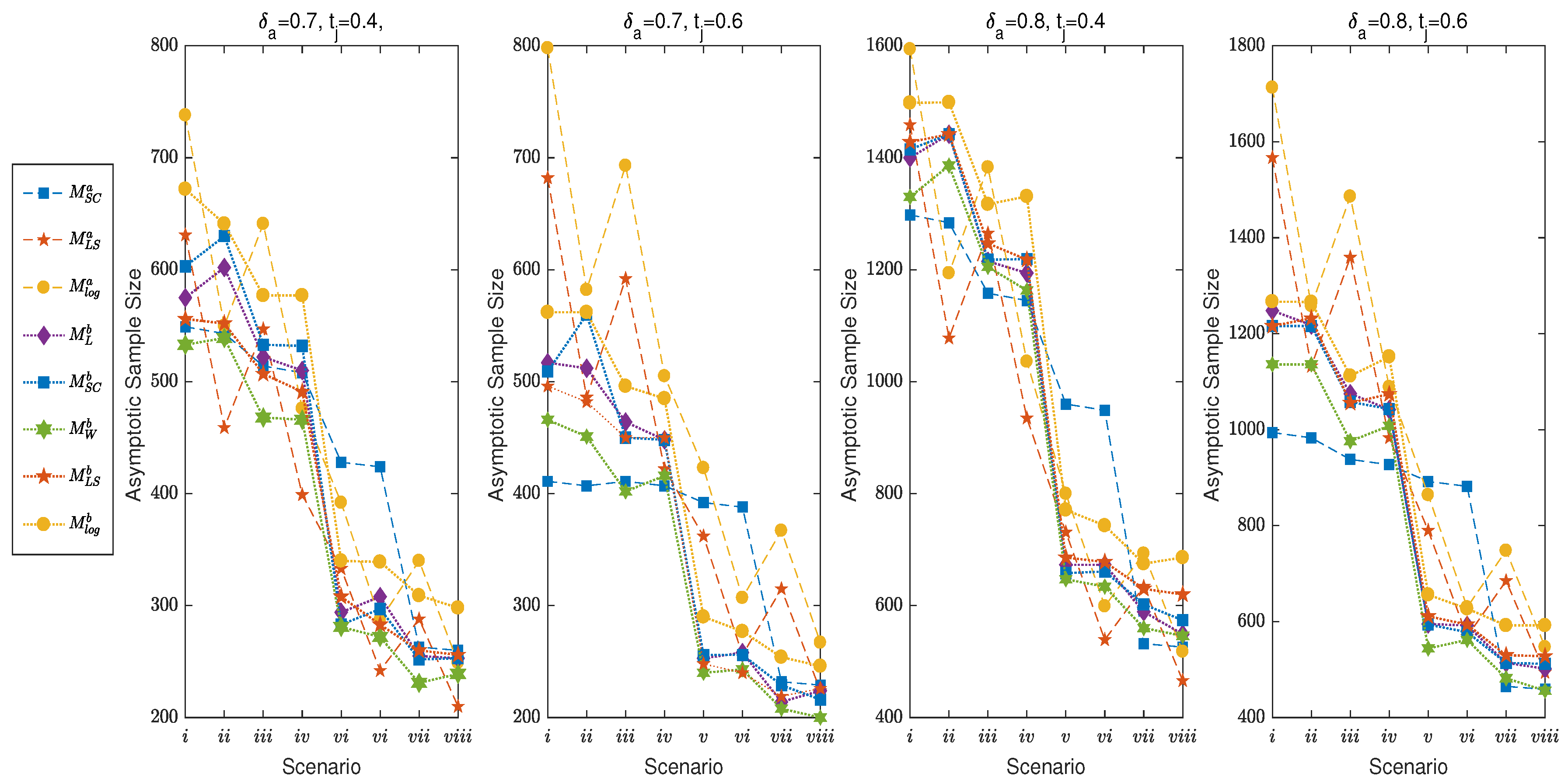
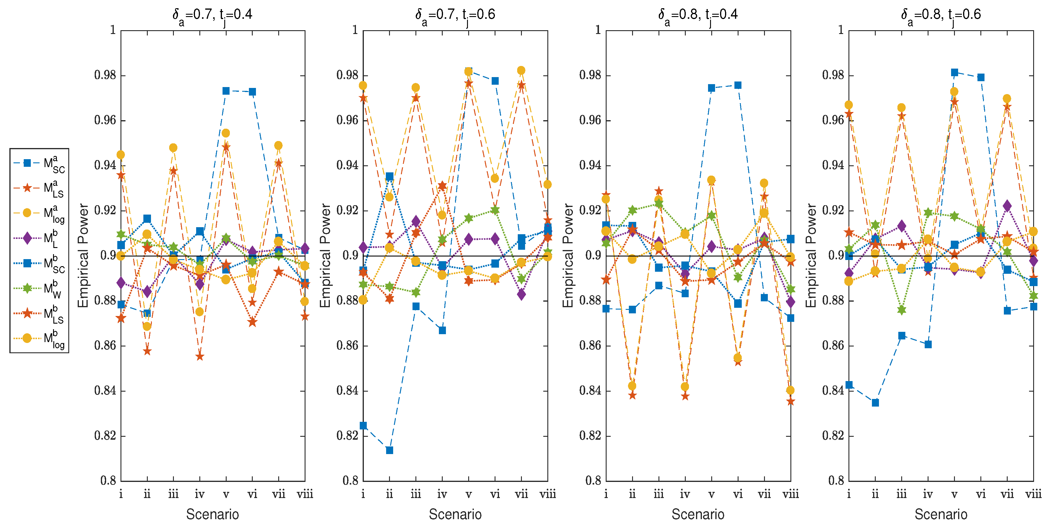
4.1. Asymptotic Sample Size, Power and TIE

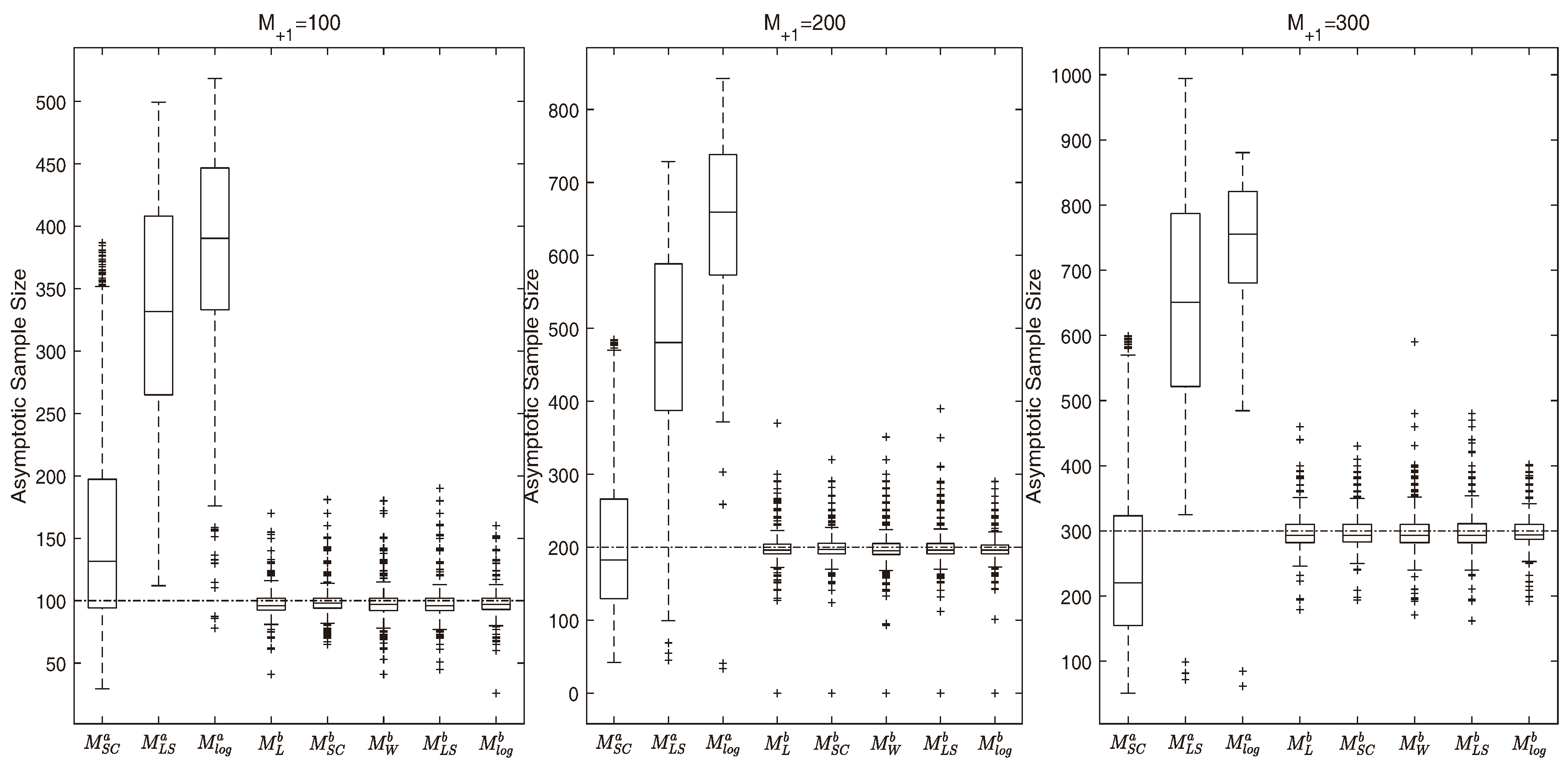
Take $J=3$. Under the null hypothesis $H_0:\delta =1$, we calculate the sample size $M_{SC}^a,M_{LS}^a,M_{log}^a,M_L^b,M_{SC}^b,M_W^b,M_{LS}^b$, and $M_{log}^b$ for given power $1-\beta =0.9$. Considering that the total numbers of strata may be the same or different, we let $\mathit{k}=(1/3,1/3,1/3)$ and $(0.5,0.3,0.2)$. The correlation coefficient ${\rho }_j=0.3$ (low), or 0.5 (moderate), and the response rates ${\pi }_{1j}=0.4$ (less than 50%), or $0.6$ (bigger than 50%). The scenarios of parameter settings in the simulations are listed in

Table 3. The scenarios of parameter settings in the simulations.

Scenario	${\mathit{\pi }}_{1\mathit{j}}$	${\mathit{\rho }}_{\mathit{j}}$	k
i	0.4	0.5	(1/3, 1/3, 1/3)
$ii$	0.4	0.5	(0.5, 0.3, 0.2)
$iii$	0.4	0.3	(1/3, 1/3, 1/3)
$iv$	0.4	0.3	(0.5, 0.3, 0.2)
v	0.6	0.5	(1/3, 1/3, 1/3)
$vi$	0.6	0.5	(0.5, 0.3, 0.2)
$vii$	0.6	0.3	(1/3, 1/3, 1/3)
$viii$	0.6	0.3	(0.5, 0.3, 0.2)

Scenarios i–$viii$ represent various parameter combinations of ${\pi }_{1j}$, ${\rho }_j$ and $\mathit{k}$.

.

Figure 1, Figure 2 and Figure 3 show the estimated sample sizes, empirical powers and TIEs of $M_{SC}^a$,$M_{LS}^a$, $M_{log}^a$, $M_L^b$, $M_{SC}^b$, $M_W^b$, $M_{LS}^b$ and $M_{log}^b$ for the given parameters listed in Table 3. We observe that there are obvious differences among $M_{SC}^a$, $M_{LS}^a$, and $M_{log}^a$ even though they are all solved by fitting asymptotic ${\chi }^2$ distributions. Asymptotic sample sizes based on the statistics $T_L$, $T_{SC}$, and $T_{LS}$ are close under the iterative method. For the five sample sizes from the iterative algorithm, the values of $M_W^b$ are always lower, and those of $M_{log}^b$ tend to be bigger. The sample sizes of ${\delta }_a=0.7$ are smaller than that of ${\delta }_a=0.8$. When other parameters are fixed, we can observe two phenomena: (i) the sample sizes become bigger for ${\rho }_j=0.5$ than ${\rho }_j=0.3$; (ii) the sample sizes tend to decrease when ${\pi }_{1j}$ increases from 0.4 to 0.6. The sample sizes increase as ${\delta }_a$ is closer to 1. That is to say, more samples are required when $\delta ={\delta }_a$ is closer to that under $H_0:\delta ={\delta }_0$.

We can calculate the empirical powers and TIEs based on the estimated sample sizes. For every sample size, 10,000 replicates ${\mathit{m}}_{ij}={(m_{0ij},m_{1ij},m_{2ij})}^T$ are randomly generated under $H_a$. Further, the empirical power can be computed by dividing the number of times rejecting $H_0$ by 10,000 when the significance level is 0.05. Empirical TIE is calculated through 10,000 replicates randomly generated under $\delta ={\delta }_0$. The results are listed in Figure 2 and Figure 3. The empirical powers are mostly close to the desired powers of 0.9. Compared with the sample size formula, the iterative algorithm often produces the sample size with empirical power closer to 0.9. In terms of empirical power, there are no significant trend changes for various parameter settings of ${\delta }_a,k_j,t_j,{\pi }_{1j}$ and ${\rho }_j$$(j=1,2,\dots ,J)$.

According to Tang et al. [8], a test is robust if its empirical TIE is between 0.04 and 0.06 when the significance level is 0.05, liberal if it is greater than 0.06, and conservative if it is less than 0.04. As shown in Figure 3, the sample size $M_{SC}^a$ has better performance in empirical TIEs. For the sample size $M_{SC}^a$, the empirical TIEs are located on $[0.04,0.06]$ under all considered settings. For some cases, the empirical TIEs based on statistics $T_{LS}$ and $T_{log}$ are lower than 0.04, which means that $T_{LS}$ and $T_{log}$ have conservative TIEs based on sample sizes from the approximate formula or the iterative algorithm. Sample sizes $M_L^b,M_{SC}^b$, and $M_W^b$ sometimes have liberal TIEs bigger than 0.06.

4.2. Accuracy

This section evaluates the effectiveness of sample size determinations. Let $J=3$, ${\delta }_0=1$, and the sample size $M_{+1}=100,200,300$. Other parameters $k_i$, ${\pi }_{ij}$, ${\rho }_j$ are randomly generated under $H_a:\delta ={\delta }_a(\ne {\delta }_0)$, satisfying $0<k_i<1,0\le {\pi }_{ij}\le 1$, $-1\le {\rho }_j\le 1$ and $0\le {\delta }_a\le 1$. Denote $\mathit{k}=(k_1,k_2,k_3),t_1=t_2=t_3,{\mathit{\pi }}_1={({\pi }_{11},{\pi }_{12},{\pi }_{13})}^T,\mathit{\rho }={({\rho }_1,{\rho }_2,{\rho }_3)}^T$. We choose 1000 parameter settings for every sample size. There are 10,000 random replications under every parameter setting. Empirical powers are given at a significance level of 0.05. Further, we calculate the corresponding asymptotic sample sizes for the obtained empirical powers at a significance level $\alpha =0.05$. The boxplots in Figure 4 show all asymptotic sample sizes.

We note that the estimated sample sizes ($M_L^b,M_{SC}^b,M_W^b,M_{LS}^b,$ and $M_{log}^b$) are close to the true sample size for $M_{+1}=100,200,300$, which performs better than the sample size formula method ($M_{SC}^a,M_{LS}^a$ and $M_{log}^a$). In terms of the sample size formula, the sample size from the score statistic is more accurate than the statistics $T_{LS}$ and $T_{log}$. The estimated sample sizes $M_{LS}^a$ and $M_{log}^a$ are always bigger than the true values. Thus, the stratified correlated model performs better for effectively estimating sample size through formula derivation.

Above all, all power-controlled methods can provide optimal estimates because the empirical powers are usually close to the prespecified one. The sample sizes from the iterative algorithm have more satisfactory power. Thus, the iterative method is recommended in practice.

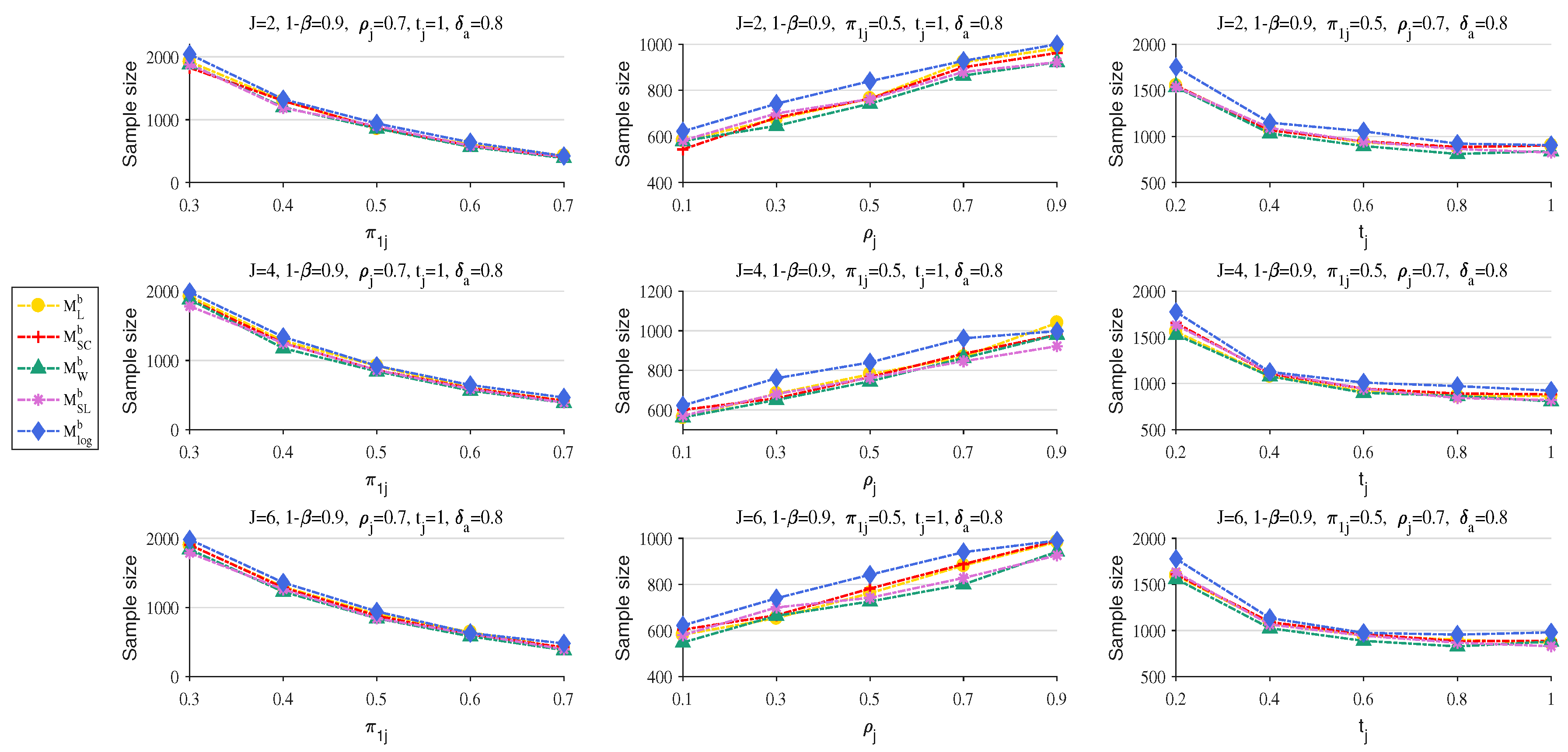
4.3. The Effect of Parameters

Through the iterative algorithm, we further study the effect of parameters on sample sizes. Given a prespecified power of 0.9 and a significance level of 0.05, the hypotheses $H_0:{\delta }_0=1$ and $H_1:{\delta }_a=0.8$. To study the effect of strata, we take $J=2,4,6$. The influence of ${\pi }_{1j}$, ${\rho }_j$ and $t_j$ can be observed according to these cases: (i) ${\pi }_{1j}=0.3(0.1)0.7$ for ${\rho }_j=0.7$ and $t_j=1$; (ii) ${\rho }_j=0.1(0.2)0.9$ for ${\pi }_{1j}=0.5$ and $t_j=1$; and (iii) $t_j=0.2(0.2)1$ for ${\pi }_{1j}=0.5$ and ${\rho }_j=0.7$. Under various parameter settings, Figure 5 shows that the asymptotic sample sizes become smaller when ${\pi }_{1j}$$(j=1,2,\dots ,J)$ increases. The five sample sizes increase with bigger ${\rho }_j$$(j=1,2,\dots ,J)$. As $t_j(j=1,2,\dots ,J)$ approaches 1, the values of asymptotic sample sizes will be smaller. This reflects that the balanced design (i.e., $N_{1j}=N_{2j}$ for $j=1,2,\dots ,J$) of two groups needs a smaller sample size for the prespecified power. When the number of strata changes, the sample sizes have similar values for $J=2,4,6$. Strata number has little effect on sample sizes.

5. A Real Example

Mandel et al. [21] conducted a double-blinded clinical trial to illustrate the proposed sample size considerations. In this trial, children with otitis media with effusion (OME) were stratified by age and randomly assigned to the cefaclor or amoxicillin treatment groups. There are three strata (<2, 2–5 and >5 yr) divided according to age as shown in

Table 4. Frequency of OME-free ears after treatment.

Number of OME-Free Ears	<2 yr		2–5 yr		>5 yr		Total
	Cefaclor	Amoxicillin	Cefaclor	Amoxicillin	Cefaclor	Amoxicillin
0	8	11	6	3	0	1	29
1	2	2	6	1	1	0	12
2	8	2	10	5	3	6	34
Total	18	15	22	9	4	7	75

.

From Table 4, it is obvious that $k_1=(18+15)/75=33/75$, $k_2=(22+9)/75=31/75$, $k_3=(4+7)/75=11/75$. Let $t_j=M_{+2}/M_{+1}=(18+22+4)/(15+9+7)=1.4$ for $j=1,2,3$. The Fisher scoring algorithm can derive the global MLEs under $H_a:{\delta }_1={\delta }_2={\delta }_3\triangleq \delta$ (see in

Table 5. Global MLEs in the real example.

Age	Stratum $(\mathit{j})$	${\widehat{\mathit{\pi }}}_{1\mathit{j}}$	${\widehat{\mathit{\rho }}}_{\mathit{j}}$	$\widehat{{\mathit{\delta }}_{\mathit{j}}}$
<2 yr	1	0.377	0.736	0.937
2–5 yr	2	0.606	0.532	0.937
>5 yr	3	0.885	0.624	0.937

). The asymptotic sample sizes are obtained based on the global MLEs of parameters ${\rho }_j,{\pi }_{1j}$ and $\delta$$(j=1,2,3)$.

Table 6. Asymptotic sample sizes for the real example.

${\mathit{\delta }}_0$	Power	${\mathit{M}}_{\mathit{SC}}^{\mathit{a}}$	${\mathit{M}}_{\mathit{LS}}^{\mathit{a}}$	${\mathit{M}}_{\mathit{log}}^{\mathit{a}}$	${\mathit{M}}_{\mathit{L}}^{\mathit{b}}$	${\mathit{M}}_{\mathit{SC}}^{\mathit{b}}$	${\mathit{M}}_{\mathit{W}}^{\mathit{b}}$	${\mathit{M}}_{\mathit{LS}}^{\mathit{b}}$	${\mathit{M}}_{\mathit{log}}^{\mathit{b}}$
0.5	0.80	70	127	67	43	43	53	86	53
	0.90	81	153	82	53	62	72	100	77
	0.95	88	170	91	70	74	86	122	94
0.6	0.80	129	213	134	77	79	91	151	120
	0.90	151	259	163	100	110	122	182	154
	0.95	164	285	180	132	132	146	218	192

shows the asymptotic sample sizes for the prespecified power $0.8,0.9$, and $0.95$ under ${\delta }_0=0.5,0.6$. The sample sizes based on $T_{LS}$ have bigger values than other sample size formulae or the iterative methods. The sample sizes from the iterative algorithm are smaller than those from the sample size formula. For ${\delta }_0$ = 0.5, the sample size 75 in the real example is close to the values of $M_{SC}^b$ and $M_L^b$ even when the power is 0.95. However, only $M_{SC}^b$ and $M_L^b$ for power 0.8 are close to the real sample size for ${\delta }_0=0.6$. That is to say, the sample size 75 can basically guarantee the power of 0.95 for the test statistics $T_L$ and $T_{SC}$ under $H_0:\delta =0.5$. Moreover, when the values of $\delta$ under $H_a$ and $H_0$ become closer, we need the larger sample size to keep the power at the fixed significance level. Then, we conduct the common test under the null hypothesis $H_0:\delta =0.5,0.6$. The values and p-values of the test statistics are recorded in

Table 7. Values and p-values of the test statistics for the real example.

${\mathit{\delta }}_0$	Result	${\mathit{T}}_{\mathit{L}}$	${\mathit{T}}_{\mathit{SC}}$	${\mathit{T}}_{\mathit{W}}$	${\mathit{T}}_{\mathit{LS}}$	${\mathit{T}}_{\mathit{log}}$
0.5	Value	8.8475	6.9551	8.2666	4.2853	4.6490
	p-value	0.0029	0.0084	0.0040	0.0384	0.0311
0.6	Value	4.3363	3.8767	4.9158	1.6514	1.7826
	p-value	0.0373	0.0490	0.0266	0.1988	0.1818

. For ${\delta }_0$ = 0.5, the p-values of five statistics $T_i(L,SC,W,LS,log)$ are 0.0029, 0.0084, 0.0040, 0.0384, and 0.0311, respectively. Obviously, the p-values are lower than 0.05. Thus, we have full evidence to reject $H_0:\delta =0.5$ at the significance level 0.05. Under $H_0:\delta =0.6$, there are some p-values smaller than 0.05 but others bigger than 0.05. Among the estimated sample sizes, only $M_L^b$ and $M_{SC}^b$ have close values to real sample sizes given power 0.8. Since p-values of $T_L$ and $T_{SC}$ are 0.0373 and 0.0490, the hypothesis $H_0:\delta =0.6$ is rejected at the significance level 0.05.

6. Conclusions

This paper mainly investigated the asymptotic sample size for the common test of relative risk ratio in stratified bilateral data. Under Donner’s model, we obtained the sample size formula and proposed the iterative method based on the likelihood ratio statistic $T_L$, score statistic $T_{SC}$, and Wald-type statistic $T_W$. We also applied the sample size methods to the pooled MLE-based Wald-type statistic $T_{LS}$ and the log-transformation $T_{log}$.

Numerical simulations are designed to evaluate the performance of estimated sample sizes. According to the simulations, the main conclusions lie in five aspects. (i) The estimated sample sizes have empirical power closer to the prespecified power level. (ii) The sample sizes $M_L^b,M_{SC}^b,M_W^b,M_{LS}^b$ and $M_{log}^b$, which are obtained by the iterative algorithm, outperform other asymptotic sample sizes because of accurate values and satisfactory power. (iii) The sample size $M_{SC}^a$ has more robust TIEs than $M_{LS}^a$ and $M_{log}^a$ from the sample size formula. (iv) The sample sizes are sensitive to ${\pi }_{1j}$ and ${\rho }_j$ ($j=1,2,\dots ,J$) when other parameters are fixed. (v) The sample sizes under unbalanced designs of two groups are greater than those under balanced designs for given power and significance levels.

This paper mainly focuses on the power-controlled sample size of the common test of relative risk ratios for stratified correlated bilateral data. However, one may want to calculate the necessary sample size such that the width of the $(1-\alpha )\%$ confidence interval (CI) does not exceed a prespecified quantity. This type of sample size is called CI-width controlled sample size determination [8]. In the future, we will study the CI-width controlled sample size for the relative risk ratio in stratified paired data. Through numerical simulation, we compared the performance of the proposed methods in terms of empirical TIEs and powers. An example was used to illustrate our proposed methods. However, we have not analyzed the theoretical results of the efficiency of these methods. These problems will be considered in our future works.

References

1. Rosner, B. Statistical methods in ophthalmology: An adjustment for the correlation between eyes. Biometrics 1982, 38, 105–114. [Google Scholar] [CrossRef]
2. Dallal, G. Paired Bernoulli trials. Biometrics 1988, 44, 253–257. [Google Scholar] [CrossRef]
3. Donner, A. Statistical methods in ophthalmology: An adjusted chi-square approach. Biometrics 1989, 45, 605–611. [Google Scholar] [CrossRef]
4. Tang, N.; Tang, M.; Qiu, S. Testing the equality of proportions for correlated otolaryngologic data. Comput. Stat. Data Anal. 2008, 52, 3719–3729. [Google Scholar] [CrossRef]
5. Pei, Y.; Tang, M.; Wong, W.; Tang, N. Testing equality of correlations of two paired binary responses from two treated groups in a randomized trial. J. Biopharm. Stat. 2011, 21, 511–525. [Google Scholar] [CrossRef]
6. Mou, K.; Ma, C.; Li, Z. Homogeneity test of relative risk ratios for stratified bilateral data under different algorithms. J. Appl. Stat. 2023, 50, 1060–1077. [Google Scholar] [CrossRef]
7. Tang, N.; Qiu, S. Homogeneity test, sample size determination and interval construction of difference of two proportions in stratified bilateral-sample designs. J. Stat. Plan. Inference 2012, 142, 1242–1251. [Google Scholar] [CrossRef]
8. Tang, M.; Tang, N.; Carey, V. Sample size determination for 2-step studies with dichotomous response. J. Stat. Plan. Inference 2006, 136, 1166–1180. [Google Scholar] [CrossRef]
9. Tang, M.; Tang, N.; Rosner, B. Statistical inference for correlated data in ophthalmologic studies. Stat. Med. 2006, 25, 2771–2783. [Google Scholar] [CrossRef]
10. Liu, X.; Shan, G.; Tian, L.; Ma, C. Exact methods for testing homogeneity of proportions for multiple groups of paired binary data. Commun. Stat.-Simul. C 2017, 46, 6074–6082. [Google Scholar] [CrossRef]
11. Shan, G. Exact approaches for testing non-inferiority or superiority of two incidence rates. Stat. Probab. Lett. 2014, 85, 129–134. [Google Scholar] [CrossRef]
12. Tang, N.; Qiu, S.; Tang, M.; Pei, Y. Asymptotic confidence interval construction for proportion difference in medical studies with bilateral data. Stat. Methods Med. Res. 2011, 20, 233–259. [Google Scholar] [CrossRef] [PubMed]
13. Pei, Y.; Tang, M.; Wong, W.; Gao, J. Confidence intervals for correlated proportion differences from paired data in a two-arm randomised clinical trial. Stat. Methods Med. Res. 2012, 21, 167–187. [Google Scholar] [CrossRef] [PubMed]
14. Qiu, S.; Poon, W.; Tang, M. Sample size determination for disease prevalence studies with partially validated data. Stat. Methods Med. Res. 2012, 25, 37–63. [Google Scholar] [CrossRef]
15. Qiu, S.; Zeng, X.; Tang, M.; Pei, Y. Test procedure and sample size determination for a proportion study using a doublesampling scheme with two fallible classifiers. Stat. Methods Med. Res. 2019, 28, 1019–1043. [Google Scholar] [CrossRef] [PubMed]
16. Sun, S.; Li, Z.; Jiang, H. Homogeneity test and sample size of risk difference for stratified unilateral and bilateral data. Commun. Stat.-Simul. C 2022, 1–24. [Google Scholar] [CrossRef]
17. Lloyd, C.; Ripamonti, E. comprehensive open-source library for exact required sample size in binary clinical trials. Contemp. Clin. Trials 2021, 107, 106491. [Google Scholar] [CrossRef]
18. Tang, N.; Yu, B. Bayesian sample size determination in a three-arm non-inferiority trial with binary endpoints. J. Biopharm. Stat. 2022, 32, 768–788. [Google Scholar] [CrossRef]
19. Pilz, M. Sample size calculation for one-armed clinical trials with clustered data and binary outcome. Biom. J. 2023, 28, e2300123. [Google Scholar] [CrossRef]
20. Zhuang, T.; Tian, G.; Ma, C. Homogeneity test of ratio of two proportions in stratified bilateral data. Stat. Biopharm. Res. 2019, 11, 200–209. [Google Scholar] [CrossRef]
21. Mandel, E.; Bluestone, C.; Rockette, H.; Blatter, M.; Reisinger, K.; Wucher, F.; Harper, J. Duration of effusion after antibiotic treatment for acute otitis media: Comparison of Cefaclor and Amoxicillin. Pediatr. Infect. Dis. J. 1982, 1, 310–316. [Google Scholar] [CrossRef] [PubMed]
Figure 1. Asymptotic sample size for 1 β = 0.9 .
Mathematics 11 04198 g001
Figure 2. Empirical power (%) based on estimated sample sizes for 1 β = 0.9 .
Mathematics 11 04198 g002
Figure 3. Empirical TIEs (%) based on estimated sample sizes for 1 β = 0.9 .
Mathematics 11 04198 g003
Figure 4. Sample sizes under various methods.
Mathematics 11 04198 g004
Figure 5. The effect of the parameter settings for sample size ( δ 0 = 1 , k j = 1 / J ).
Mathematics 11 04198 g005