Abstract
In design matters, mechanisms with deformable elements are a step behind those with rigid bars, particularly if dimensional synthesis is considered a fundamental part of mechanism design. For the purposes of this work, a hybrid rigid–flexible four-bar mechanism has been chosen, the input bar being a continuum tendon of constant curvature. The coupler curves are noticeably more complex but offer more possibilities than the classical rigid four-bar counterpart. One of the objectives of this work is to completely characterize the coupler curves of this hybrid rigid–flexible mechanism, determining the number and type of circuits as well as constituent branches. Another important aim is to apply optimization techniques to the dimensional synthesis of path generation. Considerable progress in finding the best design solutions can be obtained if all the acquired knowledge about the coupler curves of this hybrid mechanism is integrated into the optimization algorithm.
Keywords:
continuum rod; constant curvature; rigid–flexible mechanisms; path generation; dimensional synthesis; optimization MSC:
14H05
1. Introduction
Unlike rigid link mechanisms—where positions can be determined considering geometry and joints configuration by means of a purely kinematic analysis—compliant mechanisms require consideration of elasticity for defining their configuration [1,2]. Hence, a model of the deformation of parts of the mechanism must be considered along with forces and moments applied to the mechanism by its own actuators and the external environment. In this sense, obtaining closed-form solutions to classical kinematic problems becomes a difficult task.
Continuum mechanisms, where deformation of slender elements is the source of mobility, include open-loop devices based on a flexible backbone actuated along the length to introduce bending [3], and closed-loop systems, where multiple flexible rods and rigid bodies are coupled [4]. General-purpose approaches to their comprehensive position analysis employ numerical methods to solve statics and dynamics [5,6,7,8,9,10]. Nevertheless, certain assumptions and approximations can be sufficiently accurate to obtain useful closed-form solutions in some of those applications.
Regarding open-loop continuum mechanisms, one option is to approximate the deformed shape of elements of the mechanism using specific curves. For example, Hirose [11] employed serpenoid curves, assuming that curvature changes sinusoidally along the length, fitting well with the biological motion of snakes. Alternatively, Chirijkian [12,13] describes the backbone curves by means of shape functions that are restricted to a modal form. Then, the inverse kinematic problem reduces to determining the time-varying backbone curve behavior. Possibly the most common approach is to approximate backbone deformation as a series of arcs of constant curvature that are mutually tangent. This is a good approximation in many cases, such as active cannulas based on concentric pre-curved tubes [14]. Further, pneumatically actuated trunks [15] can behave like a piecewise constant curvature system. A comprehensive review of the state of the art on constant curvature rods can be found in [16]. Moreover, the work in [17] shows that a constant torque can be applied by means of a wire attached to the end of a flexible rod, passing through a sufficient number of guide discs fixed to the rod. The latter case, based on tendons and guide discs, is possibly the most straightforward and simplest way to implement an active flexible rod. Many continuum robots consist of a multiply actuated single member, which is capable of tracing curvilinear trajectories suitable for applications in confined spaces and tasks such as non-destructive inspection or minimally invasive surgery.
More recent works have focused on the inclusion of flexible rods in closed-loop systems (such as parallel robots) to benefit from advantages such as good maneuverability, miniaturization, low weight, and inertia. Following the rationale of parallel kinematic machines, the actuation is distributed among the parallel members and placed in the fixed frame when possible. Usually, flexible members play a passive role, and the actuation is applied to the first end-tip of rods by controlling displacement or orientation. In this regard, works focusing on continuum hexapods [18] and their implementation in surgical devices [5] have been conducted. The authors of this paper have investigated the position problem of closed-loop flexible mechanisms [19] and the multiplicity of the buckling mode of slender links on planar parallel continuum mechanisms [20]. Additionally, [21] presents a 3-DOF planar parallel continuum robot, suitable for high-precision applications, achieving nanometer repeatability.
In the aforementioned examples, flexible rods enable the movement of the mechanism, but they are not the actuating members themselves. However, active flexible rods used in open-loop continuum mechanisms can also play an active role in such parallel devices if they are implemented to actuate the mechanism. This idea has been exploited in parallel soft robot manipulators manufactured with rubber bars containing pneumatically actuated chambers [22]. Another example [23] uses a platform attached to pneumatically actuated chains made of polyimide material through spherical joints. More recently, the authors of [24] developed an approach consisting of employing tendon-driven rods to actuate parallel kinematic mechanisms. In this latter case, the kinematic analysis problem of a 3-RF[b]R parallel robot was addressed by taking advantage of the simplifications related to working with constant curvature deformable rods.
Most of the multi-degree-of-freedom flexible devices have been developed from analogies with rigid-link mechanism counterparts. Indeed, there is limited research activity in the field of dimensional synthesis [2], and much of the work related to the design of mechanisms with deformable elements is supported by the synthesis of a compliant mechanism. The main methods used to synthesize compliant mechanisms include the freedom and constraint topologies (FACT) [25,26], topology optimization [27], the practical method of rigid-body replacement [28], and the building-block approach [29]. Research on dimensional synthesis of such systems is even more scarce and is usually reduced to a limited optimization of a set of elastic parameters.
The authors of this paper are interested in studying the possibility of applying dimensional synthesis optimization methods of rigid-bar mechanisms to flexible-bar mechanisms. Precisely, the four-bar hinged linkage is undoubtedly the mechanism most used by the scientific community for its verification. It has been used for function generation, path generation, and motion generation using local, global, and hybrid optimization methods. A small sample of these works can be found in the following references: [30,31,32,33,34].
For all these reasons, in the present study, the authors selected a hybrid four-bar hinged linkage where the crank (or rocker) input has been replaced by a driven continuum rod. The dimensional synthesis of this mechanism is focused on path generation. The following abbreviated nomenclature will be used hereafter:
- RFB: Rigid Four-Bar Hinged Linkage
- FFB: Tendon-Driven Hybrid Rigid–Flexible Four-Bar.
In general, optimization procedures applied to the dimensional synthesis of mechanisms—both global and local methods—function like closed boxes. Once the optimization algorithm comes into action, the designer loses control. Our experience indicates that a good direction of descent in minimization is sometimes penalized by a default that could be easily resolved if the geometry of the path in the current iteration were known. Often, excessive use of penalty functions places too many restrictions on the design space.
Therefore, the first part of this paper is devoted to examining the trajectories of the FFB coupler point, the composition of its circuits, and the existence of one or two branches within the circuits. The results obtained reveal fundamental differences with respect to the RFB. In fact, the FFB can have “open” circuits, while paths with more than two circuits also exist; and no (closed) circuit exists with only one branch. This, in itself, constitutes a contribution toward knowledge of the paths of the FFB coupler point, like its previously studied RFB counterpart.
The second part of the article characterizes the coupler curves by incorporating these into an optimization algorithm, with two aims in mind. The first is to avoid circuit and order errors. To perform this, the optimization algorithm must know, at each iteration, in which circuit and in which branch the coupler point is located. The second aim is to integrate knowledge about the number and type of circuits that make up the path into the optimization algorithm. The idea is that the optimization algorithm itself presents tools of intelligent assistance in the search for the best solution. The significant differences between the coupler curves of the FFB and the RFB condition largely determine the optimization process of the path generation of the FFB. Therefore, in our opinion, this second part constitutes another important contribution to the existing knowledge of the dimensional synthesis of mechanisms with continuum rods.
Finally, throughout the paper, a comparison of the FFB with its rigid bar counterpart is made in order to establish analogies and differences between the two.
2. Materials and Methods
In this section, the characterization of the coupler curves of the FFB as well as the functioning of the optimization procedure are presented.
2.1. Kinematics of Continuum Rod with Uniform Curvature
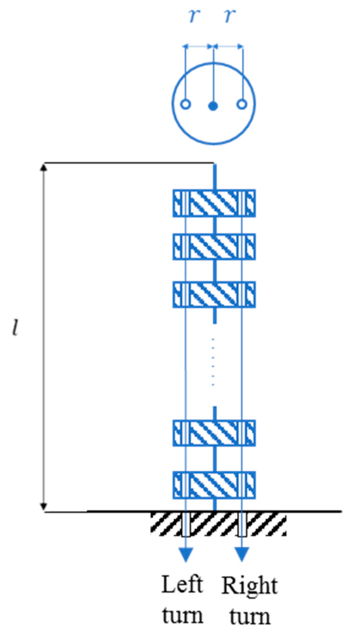
A particularly interesting flexible body, which cannot be modeled with pseudo rigid body models, is the driven continuum rod [24]. This device is composed of a series of disks connected together by a flexible central spine and two cables, as shown in Figure 1. A uniform curvature can be achieved along its entire length by picking up length in one cable and releasing the other by the same amount (Figure 2). Curvature varies with time, thus achieving motion.

Figure 1.
Cable-driven continuum rod with constant curvature.
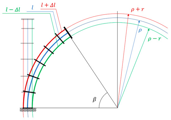
Figure 2.
Geometry of an embedded continuum rod with constant curvature.
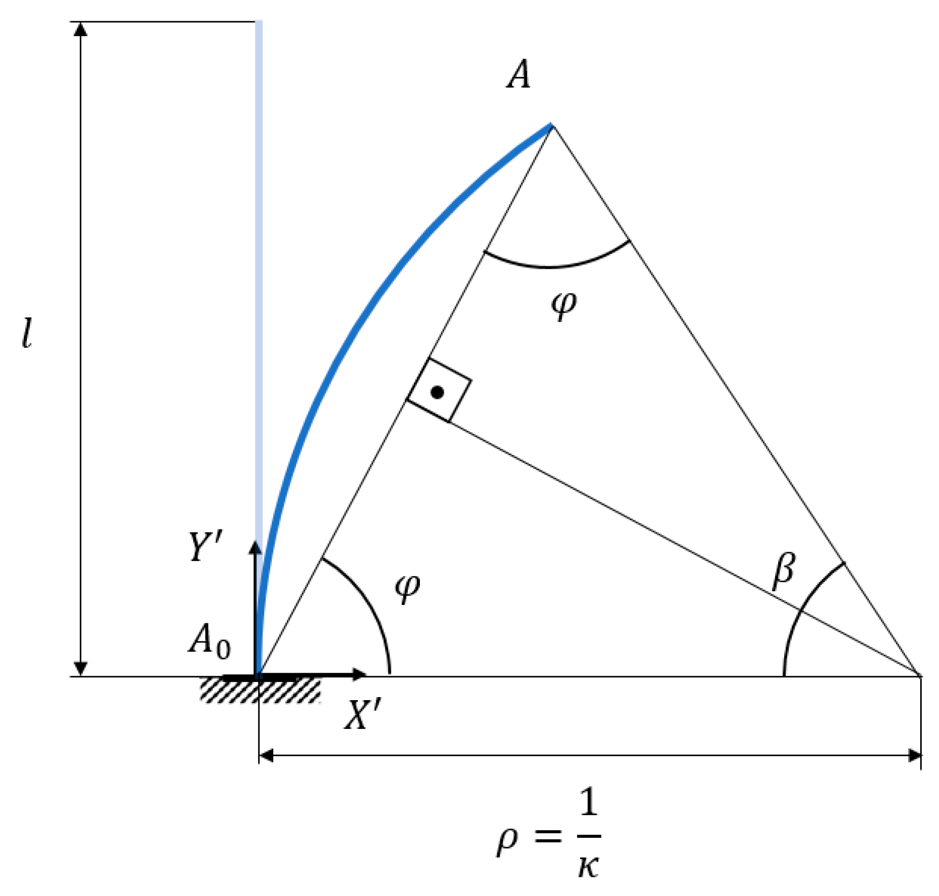
It is interesting to note here that the deformed configuration of the rod shown in Figure 3 can be described as a function of the rod length () and the curvature () by means of simple expressions, being able to integrate this element into kinematic calculations without the need to consider the forces and moments involved.
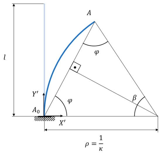
Figure 3.
Variables describing the kinematics of continuum rod.
From the geometry of Figure 3, the expressions for the coordinates of point describing the position of the rod tip in the reference frame are
If is expressed as a function of , then
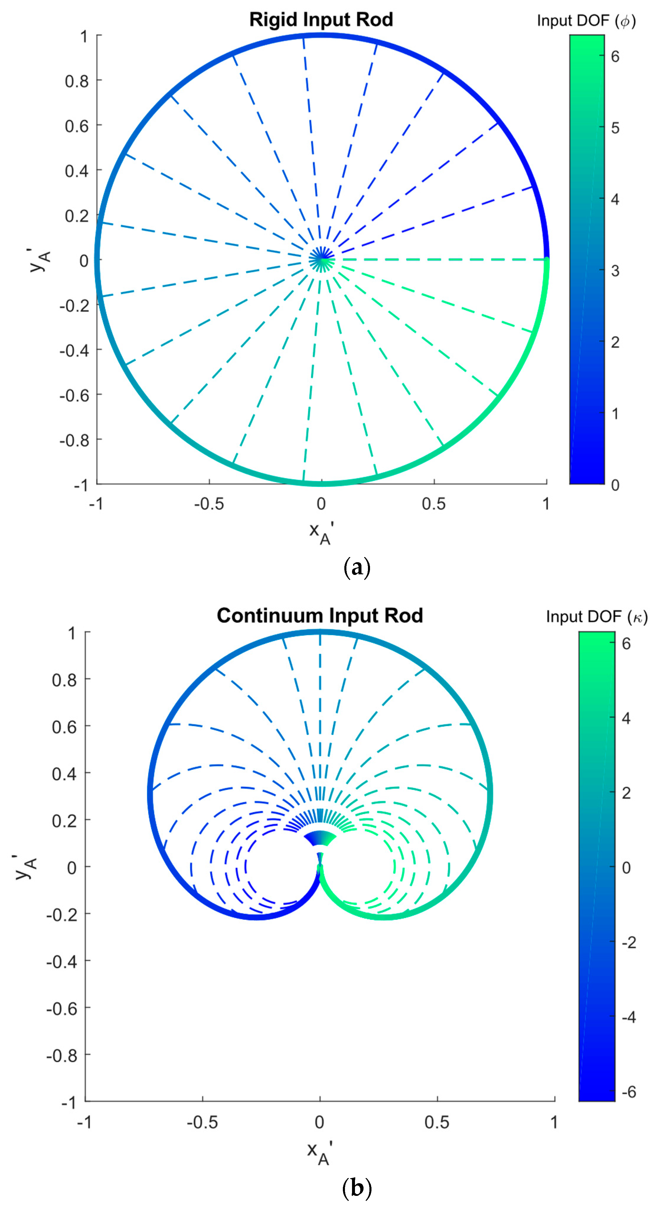
In the case of the continuum rod, when monotonically increasing or decreasing the value of input from a starting position, the connecting rod will never return to that starting position, unlike in the case of the rigid rod. Indeed, in RFB linkage, it is usual to impose the Grashof condition on the early design phase to ensure the complete rotation of the input element, since this facilitates the work of the actuator, as there are no blocking positions. However, in FFB, the input continuum rod will never behave as a fully rotating crank since its kinematic equations do not show cyclic behavior.
The aforementioned situations are depicted in Figure 4a,b, showing the displacements of two rods of unit length : the rigid and the continuum rod, respectively. These figures also represent the trajectories described by the ends of both rods for input values in the interval Consequently, as known, the RFB can have circuits composed of a single branch because the input element can make complete turns, returning to its starting configuration. However, this is not possible in a FFB, because of the concept of closed that the word “circuit” entails.
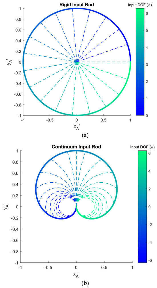
Figure 4.
Motion of input rod vs input parameter: (a) rigid input; (b) continuum input.
In the case of the continuum rod, it follows from its equations that for , the continuum rod turns back on itself, obtaining configurations that, although valid from a mathematical standpoint, lack practical interest. Since we are working with planar mechanisms, the continuum rod would interfere with itself. On the other hand, excessive curvature is not possible in a structure with cables and disks, such as the one shown in Figure 1.
2.2. Path Characterization of the Coupler Point of a FFB; Comparison with RFB
The kinematic analysis of the four-bar hinged linkage on both rigid and flexible versions will be discussed below, describing the analogies and differences between them. Figure 5 identifies the dimensional parameters and the passive variables in both rigid and flexible designs, as well as the corresponding input ( in RFB and in FFB).
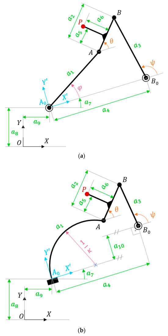
Figure 5.
Kinematic variables in (a) RFB and (b) FFB.
At a glance, we can observe two differences between them. First, the different nature of the input variables in the RFB and FFB, and , respectively, will have consequences for the complexity of the equations, particularly in the case of the FFB. Second, the RFB has 9 dimensional parameters, and the FFB has 10. The additional dimensional parameter of the FFB () defines the offset between the fixed joint and the floor of the continuum rod embedment.
To characterize the FFB coupler curves, it is necessary to solve the position problem. This characterization does not depend on operations such as translation and rotation of the mechanism, and thus, the coupler curve can be determined in the local reference frame . Considering Equations (5) and (6) of the continuum rod and projecting the loop equation of the FFB (Figure 5b) on the axes of this local system, we obtain
By combining Equations (7) and (8), can be removed, resulting in the following equation:
where:
By isolating the variable from Equation (9), the following expression is obtained:
where:
The index in Equation (13), which has a similar meaning to that in [35,36] for the RFB linkage, can take the values ±1, giving rise to two values of . Each value of corresponds to one mechanism configuration (see Figure 6). The configurations belonging to the same branch correspond to values of obtained with the same value of . A branch can have limits or not. Beyond these limits, the variable ceases to have real values. This mathematical situation occurs when the mechanism reaches a configuration where, beyond it, the mechanism can no longer be assembled, that is, the mechanism has reached a blocking position.
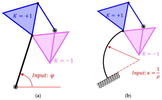
Figure 6.
The two configurations for a given value of the input: (a) RFB and (b) FFB.
2.2.1. Blocking Positions
Consider a FFB defined by a dimensional vector . Note that only these dimensions influence the branches and circuits. Indeed, and simply define the relative position of the coupler point, while , , and are responsible for the rotation and translation transformations of the mechanism.
The valid values of the input parameter are those for which the mechanism can be physically assembled. Only for those values will the passive variable take a real value. Then, the function under the root of Equation (13) must be greater than or equal to zero:
Therefore, the values of that give rise to blocking positions in FFB are those in which is null.
The blocking positions can occur for any value of the input variable. Thus, the domain to be analyzed in RFB is , while in FFB, it is .
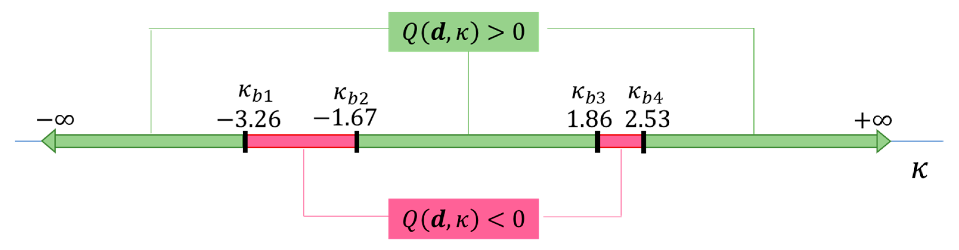
To illustrate these ideas, Example 1 of Figure 7 will be used, of which the dimensions of the corresponding mechanism are shown in Table 1. Figure 7 represents the domain of the input , showing the existence of intervals of the variable, as well as its extremes.
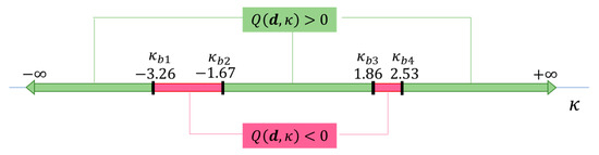
Figure 7.
Example 1. analysis for a specific FFB defined by dimension .

Table 1.
Dimensional parameters for Examples 1, 2, and 3.
As can be observed in Figure 7, three intervals verify (depicted in green color). Each contains the set of configurations through which the mechanism can move without being physically disassembled. Note that, for the FFB, the extremes are not necessarily finite values, but they may reach or . Then, extremes of the intervals can correspond to configurations whose input takes infinite value or to a blocking position. In physical terms, each interval corresponds to one circuit of the coupler curve of the mechanism. Depending on the type of extremes, the circuits are composed of one or two branches, as shown below. Intervals having an infinite extreme result in “open circuits”, which cannot occur in the RFB. Note that, although “open circuits” might sound semantically contradictory, this terminology will be kept to distinguish between these two different situations (open and closed curves).
Moreover, in the example shown in Figure 7, there are another two intervals, depicted in pink color, for which . The mechanism cannot be assembled within the ranges of these input values. The boundaries between valid and invalid input values are in fact the four blocking positions denoted in Figure 7 as , where changes sign. To better illustrate this scenario, the second blocking position, , is depicted in Figure 8, where the alignment of the bars is clearly evident, as in the case of the RFB. Figure 8 also shows how the two blocking positions delimit the two branches that make up the circuit. The first branch is obtained with the index and the second branch with .

Figure 8.
Example 1. Blocking position .
Another difference between the RFB and the FFB lies in the difficulty in obtaining the values of the input variable at which the blocking positions occur. In an RFB, these are extracted analytically from a second-degree algebraic equation [36]. In contrast, in a FFB, these values are obtained from , where is a highly complex expression (see Equations (10), (11), (12), and (14)), bearing in mind that the input appears both inside and outside the trigonometric functions. Therefore, the values of associated with the blocking positions in FFB can only be extracted numerically.
2.2.2. Branches and Circuits in the FFB Coupler Curves
In an RFB, closed circuits are always obtained, which may be composed of one or two branches depending on the range of motion of the input in each circuit:
- For a crank input, two circuits will always exist, each one composed of one unique branch.
- For a rocker input, there may be one or two circuits. Each circuit has two branches, which are connected at blocking positions.
While a FFB shares certain similarities with an RBF, significant differences also appear due to Equation (15). On the one hand, each circuit may be composed of one or two branches. On the other hand, each circuit can be “open” or closed depending on the range of motion of the input . The following three cases can be distinguished:
- Case I: If the range is bound by two blocking positions, i.e., two finite values of this leads to a closed circuit with two branches.
- Case II: If the range has one single blocking position, i.e., it is bound by a finite value while the other extreme is or , this leads to an open circuit with two branches.
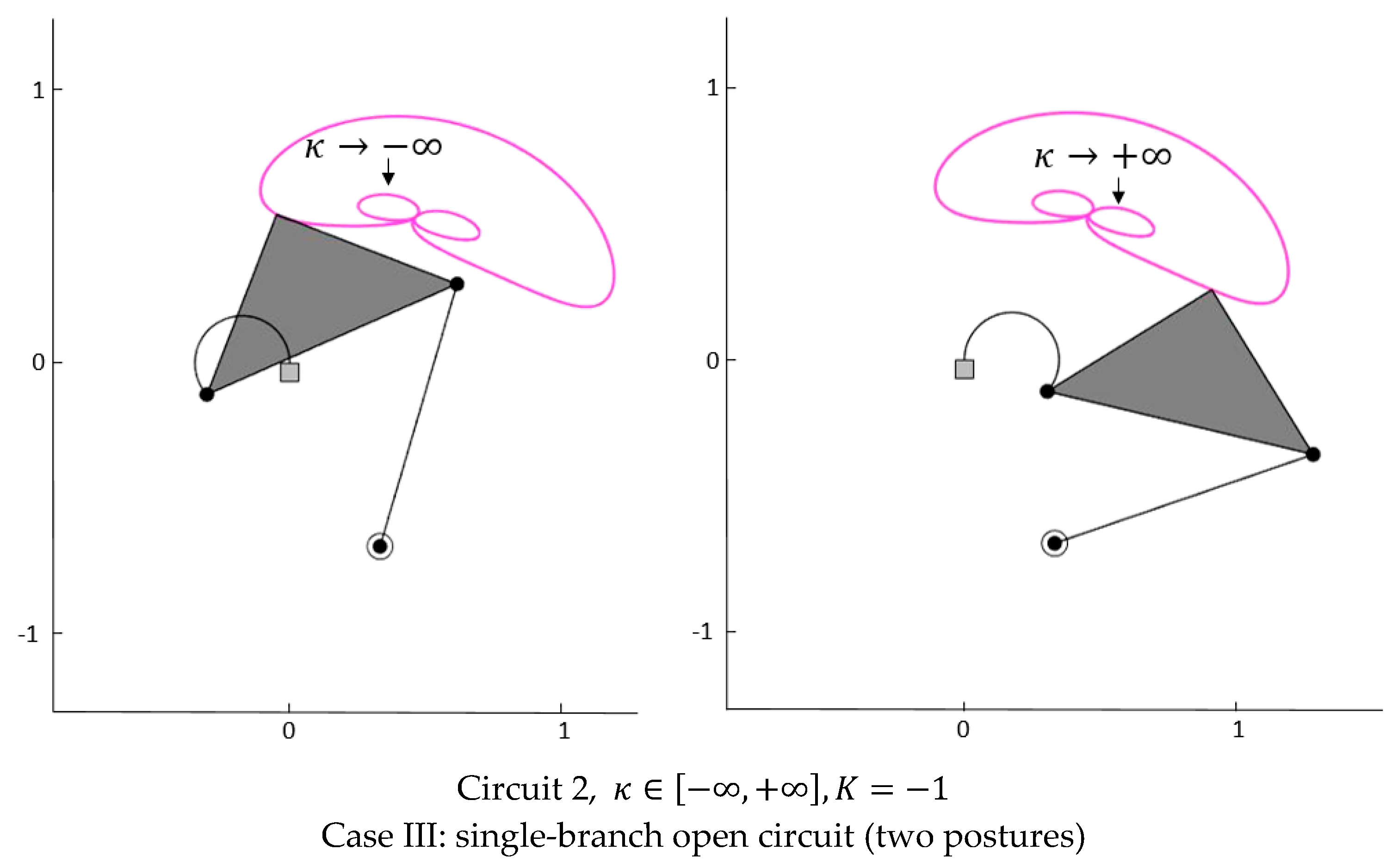
- Case III: If the whole range is valid, there are no blocking positions, and two single-branch open circuits are obtained.
In the light of these three cases, further differences between an RFB and a FFB can be pointed out. First, as long as the curvature is the input variable—which is the premise of this work—single-branch closed circuits cannot be obtained since is not a cyclic variable, unlike in the case of the RFB. Second, in Case II, the curvature increases to infinity without reaching the blocking position, so that the coupler curve reaches its end point when or without closing. These types of positions are not achievable in practical applications, since the rod would suffer a significant bending moment and eventually break. Moreover, for , the rod would interfere with itself, assuming an in-plane motion. Furthermore, with respect to the solutions of Equation (15), a mechanism may give rise to several intervals of valid input values, each of which will correspond to a circuit that may fall into any of the three typified cases. Consequently, a mechanism may have multiple circuits that can be open or closed, some with two branches and some having only one. Unlike in an RFB, where there can be a maximum of two circuits, in a FFB, many more can be obtained. These conclusions will be illustrated subsequently with several examples.
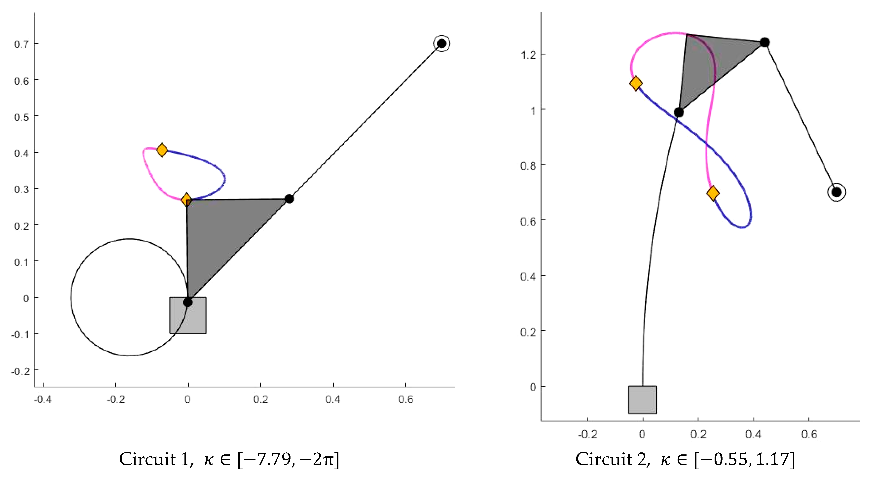
Continuing with the previous Example 1, this mechanism has a coupler curve with three circuits, as represented in Figure 9. Two of the circuits correspond to Case II, and the remaining one to Case I. In this example (as in subsequent ones), the first branch is obtained with index and the second branch with .
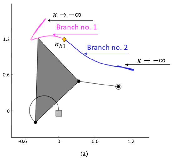
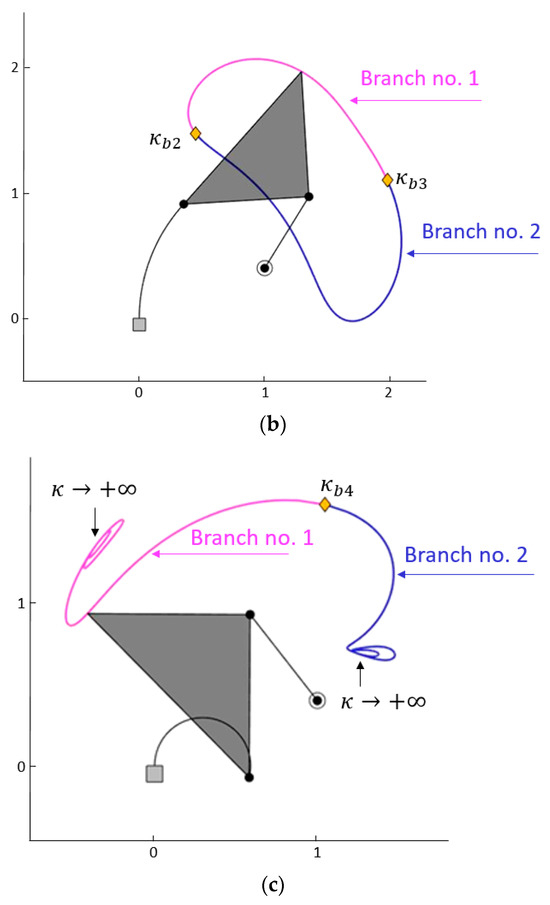
Figure 9.
Example 1. Three circuits associated with Cases I and II. (a) Circuit 1, ; Case II: open circuit, two branches. (b) Circuit 2, ; Case I: closed circuit, two branches. (c) Circuit 3, ; Case II: open circuit, two branches.
To illustrate Case III, the mechanism of Example 2, shown in Figure 10, will be used. The corresponding dimensional parameters are listed in Table 1. As can be observed, in this second example, the curvature takes valid values in the whole domain. The coupler curve is composed of two single-branch open circuits. It is worth noting, in this case, that if the ideal non-practical values of κ were accepted, and , the extremes of each single-branch open circuit, corresponding to the values and , would coincide. In this sense, it appears that the circuit becomes closed. However, we prefer to be consistent with what has been described so far, and not consider impractical values of κ. Therefore, we will assume that the circuits are open.
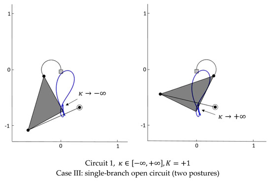
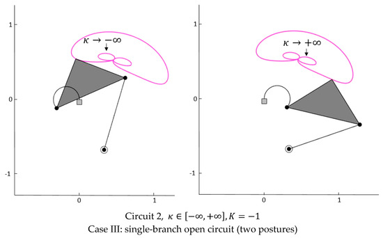
Figure 10.
Example 2. Two circuits associated with Case III.
The maximum number of circuits in a FFB still remains to be verified, since this is directly related to the maximum number of real solutions of Equation (15). The extreme complexity of this equation has already been pointed out. It is probable that in an equation of this mathematical complexity it is not possible to determine the maximum number of real solutions and, therefore, the maximum number of blocking positions and circuits. This contrasts with the well-established maximum of 2 circuits in the RFB. Nevertheless, the authors conducted an automatic study on FFB linkages, obtained by randomly combining the components of dimensional vector . This study established a maximum of 4 circuits within the practical utility domain . Extending this study to the whole domain yielded a maximum of 10 circuits.
Figure 11 shows a new example (Example 3) with 4 closed circuits, each with two branches. The dimensions of the mechanism corresponding to this third example are listed in Table 1. Despite having four circuits, it is worth noting that Circuits 1 and 4 are not entirely useful in practice. In the case of Circuit 1, the values are of no interest, as they lie outside the aforementioned domain of practical utility. The same occurs for Circuit 4, with the interval .

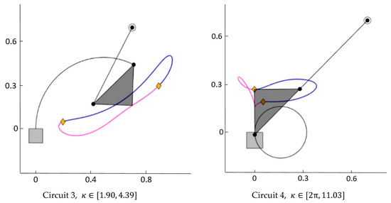
Figure 11.
Example 3. Four circuits.
2.3. Optimization Method for Path Generation of a FFB
This section will describe a methodology for the dimensional synthesis of FFB path generation. This methodology can be easily adapted to the cases of function and motion generation.
The coordinates of the coupler point of the FFB (Figure 5b), which refer to the global frame , can be expressed as follows:
where are the coordinates of the coupler point referring to the local system :
By adopting the sum of squared distances between generated and prescribed points as the error function , then
being the number of the precision points of the prescribed trajectory.
From here on, the main steps of the optimization procedure proposed in [35] will be followed, but by incorporating the knowledge acquired regarding the branches and circuits of the FFB, as will be explained in subsequent sections. Therefore, in this work, only those aspects of this procedure that the authors consider essential for its understanding will be indicated. Note that, since this procedure follows a local optimization, the choice of an initial design is a relevant step and will have an important effect on the quality of the solution obtained. In our case, a candidate mechanism is manually identified, and can be used directly in the initial iteration, or can be manually adjusted by “trial and error” to try to improve the quality of the approach.
It is essential to obtain the derivatives of the synthesis equations, in our case Equations (16) and (17), with respect to each of the dimensional parameters and the input variable . By following the tree derivation rule, according to the functional dependence law, implicit derivatives of the type and appear, which are the most difficult to obtain. In this case, instead of deriving Equations (7) and (8) implicitly, it is simpler to derive Equation (13) explicitly but taking into account the functional dependencies of , and with respect to and .
2.3.1. Incorporating Knowledge of FFB Branches and Circuits into Path-Generation Synthesis; Avoiding Circuit Error
At each iteration of the synthesis process, it is necessary to construct the map of circuits and branches of the mechanism. With the input of each generated point , it is possible to determine the circuit of the mechanism in which it is located. To evaluate the position of a generated point with respect to its corresponding prescribed point , it is sufficient to obtain from Equation (13) the two values of the passive variable and enter these into the synthesis Equations (16) and (17), and then place the two solutions on the circuit or circuits at the current iteration mechanism. From here on, any of the cases described in Section 3.2 can be treated as follows:
- Case I: A closed circuit with two branches. The values of the index give rise to two solutions, one in each branch. Clearly, the one with the smallest distance from the prescribed point must be taken. Once the branch is detected, the rest of the points of the synthesis are evaluated on the same branch (with the same value of ). By adopting this approach, the order error is avoided.
- Case II: An open circuit with two branches. The functioning is the same as in the previous case.
- Case III: Two single-branch open circuits. In this case, the index values determine both the branch and the circuit. As in Cases I and II, the value of with the smallest distance from the prescribed point is selected. This determines the circuit in which the synthesis has to be performed, thus avoiding the circuit error.
Note that, in cases where it is possible to pass through the blocking positions, the procedure could work with points belonging to the two branches, provided that both are part of the same circuit (Cases I and II). One way to pass through a blocking position is to transiently change the input to the rigid bar and then immediately return the actuation to the tendon.
2.3.2. Avoiding Order Error
Order error occurs when the coupler point of the mechanism resulting from the synthesis does not follow the previously established ordered sequence of prescribed points. When a circuit is composed of a single branch (Case III), it is very easy to avoid the order error: it is sufficient to assign to the prescribed points an ordered sequence of input parameter values in increasing (or decreasing) order. Clearly, all the points generated must have the same index value.
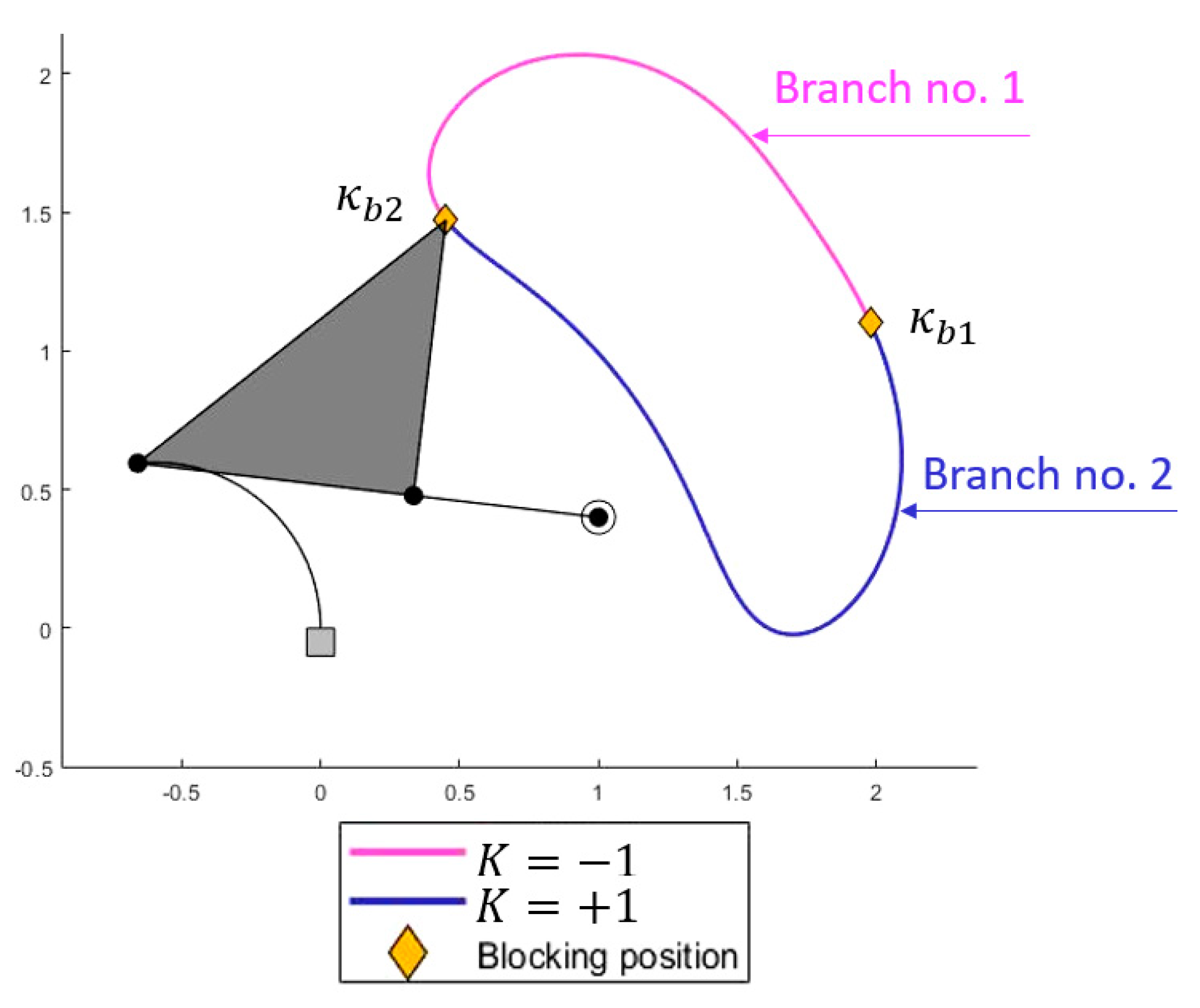
For the remaining cases (I and II), where the circuits consist of two branches, avoiding order error can be achieved as follows. For case II (open circuit with two branches), it is sufficient to take the ordered sequence following the direction from the blocking position to +∞ (or to −∞, depending on the branch). However, for Case I (closed circuit with two branches), to be able to use points located on both branches of the circuit, it will be necessary to follow the strategy represented in Figure 12.
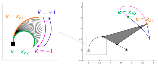
Figure 12.
Illustrative example demonstrating how to avoid order error.
Figure 12 represents a circuit with two branches, separated by the blocking positions and . The pink colored branch () is traversed in the direction of input variation from to , while the blue-colored branch () is traversed when the input goes from to . Let us assume that the ordered sequence of points to be generated by the mechanism falls on both branches, the starting point being located on the pink branch. For the mechanism to follow the ordered sequence, the continuum rod must deform clockwise to the blocking position . Then, the continuum rod reverses its input by continuing along the blue branch until it reaches the last point . The optimization algorithm is able to detect the blocking positions in which one branch is changed to another, so that the direction of the input is reversed once the boundary defined by these blocking positions is crossed. This is possible due to the acquired knowledge regarding the branches and circuits of the coupler curve of the FFB.
3. Results
In this section, two demonstrative examples of a path-generation optimum dimensional synthesis of a FFB will be shown.
3.1. Path Generation Example 1 (PG-Example1)
The data according to the prescribed points for this PG-Example1 are taken from reference [37], with the corresponding coordinates indicated in Table 2. In [37], path generation was conducted using a double butterfly mechanism (eight elements including the fixed one: four binary and four ternary) and without restriction of the input parameter (unprescribed timing).
Table 2.
Coordinates of prescribed points of the objective path in Ref. [37].
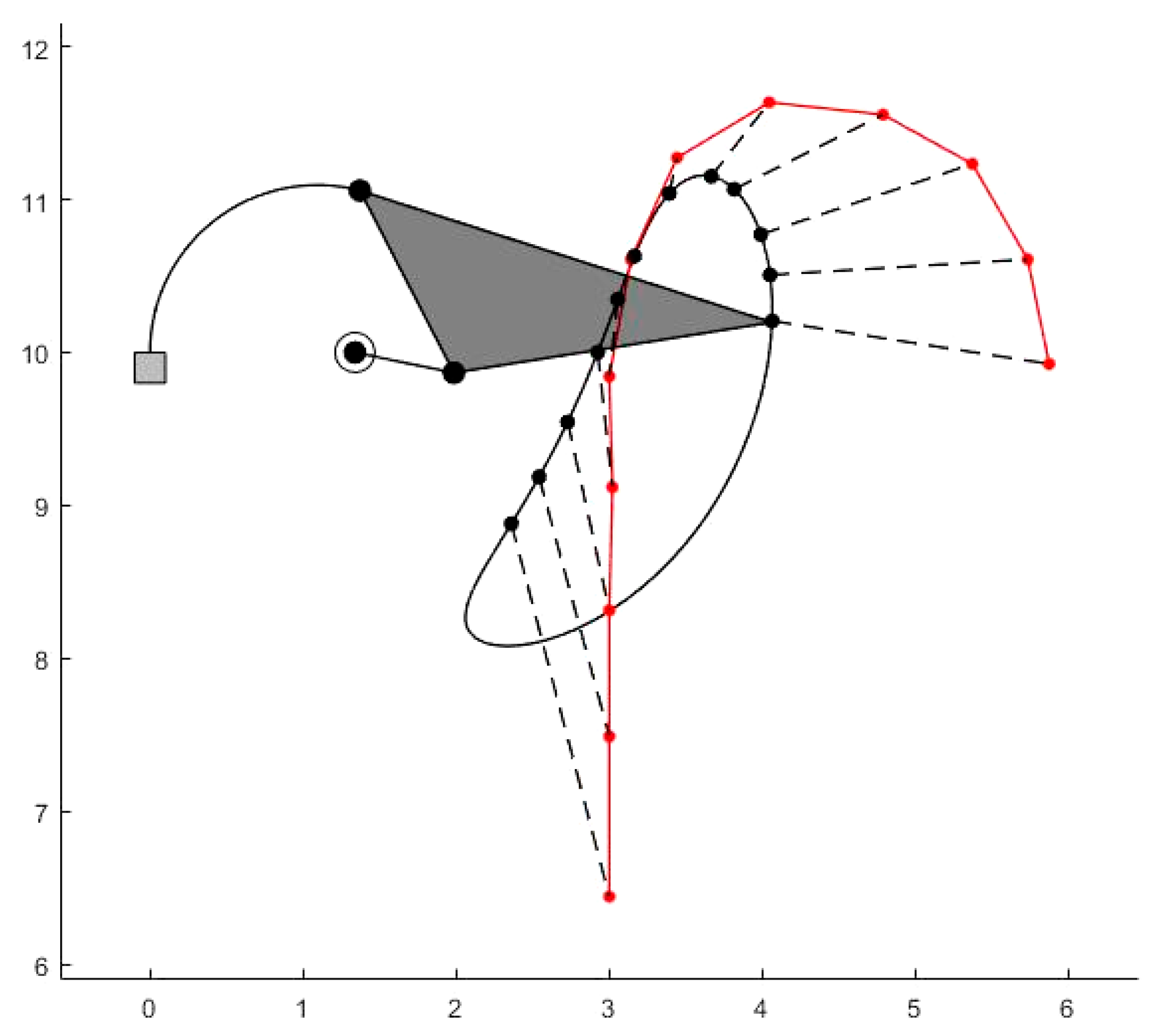
In PG-Example1, an unprescribed timing path-generation optimization with a FFB was carried out. Figure 13 and Figure 14 show, respectively, the initial guess mechanism and the optimal solution obtained. The value of the error function declines significantly from 22.02 to 0.0032 after design optimization. In both figures, the desired trajectory is depicted in red color, while the initial trajectory (Figure 13) and the obtained optimal trajectory (Figure 14) are depicted in black.

Figure 13.
PG-Example1. Starting mechanism for path generation, error = 22.02.
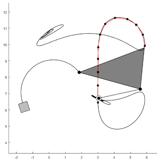
Figure 14.
PG-Example1. Optimal mechanism achieved, error = 0.0032.
Table 3 displays the dimensional parameters and input values associated with the initial and optimal solutions, respectively.
Table 3.
PG-Example1. Starting mechanism and optimal design parameters and inputs.
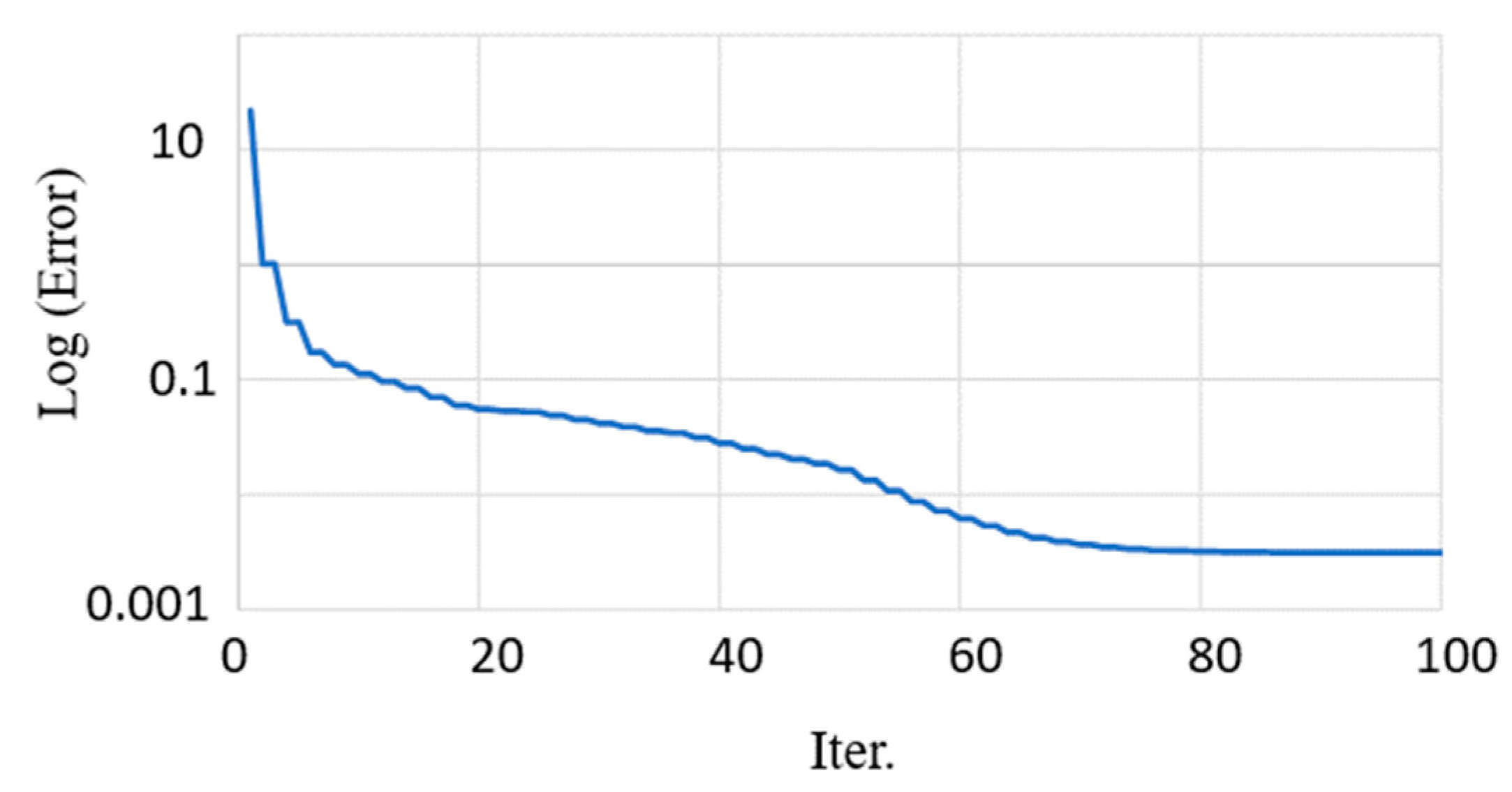
Finally, Figure 15 plots the error function against the number of iterations. Convergence to a final solution was achieved after 80 iterations, with a total computation time of just 0.5 s. Note that this and the subsequent example were solved using a mid-range laptop (Asus Zenbook, Intel Core i7 8565 U CPU @ 1.80 GHz 1.99 GHz, RAM 16 GB).

Figure 15.
PG-Example1. Convergence of optimization procedure.
3.2. Path Generation Example 2 (PG-Example2)
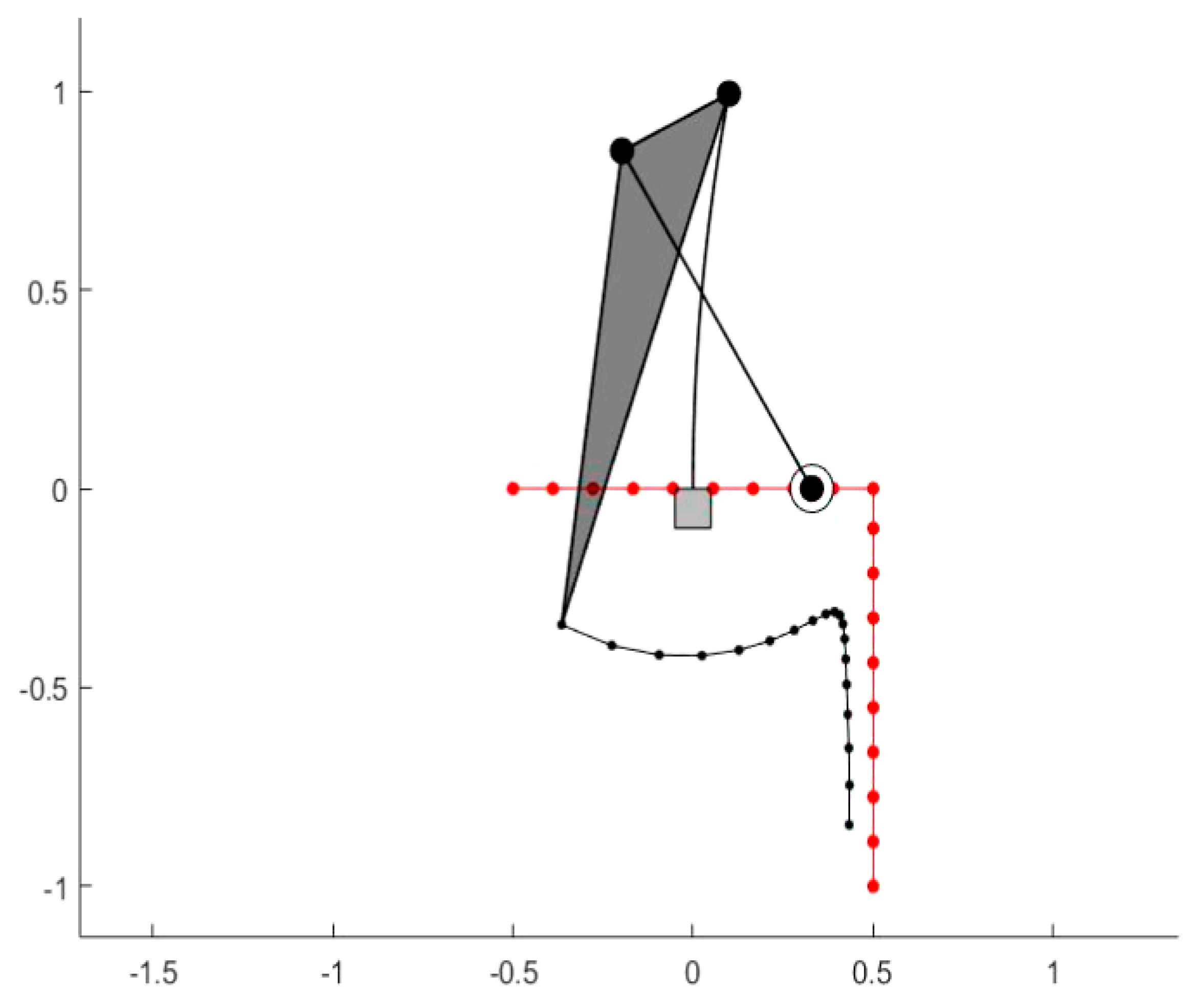
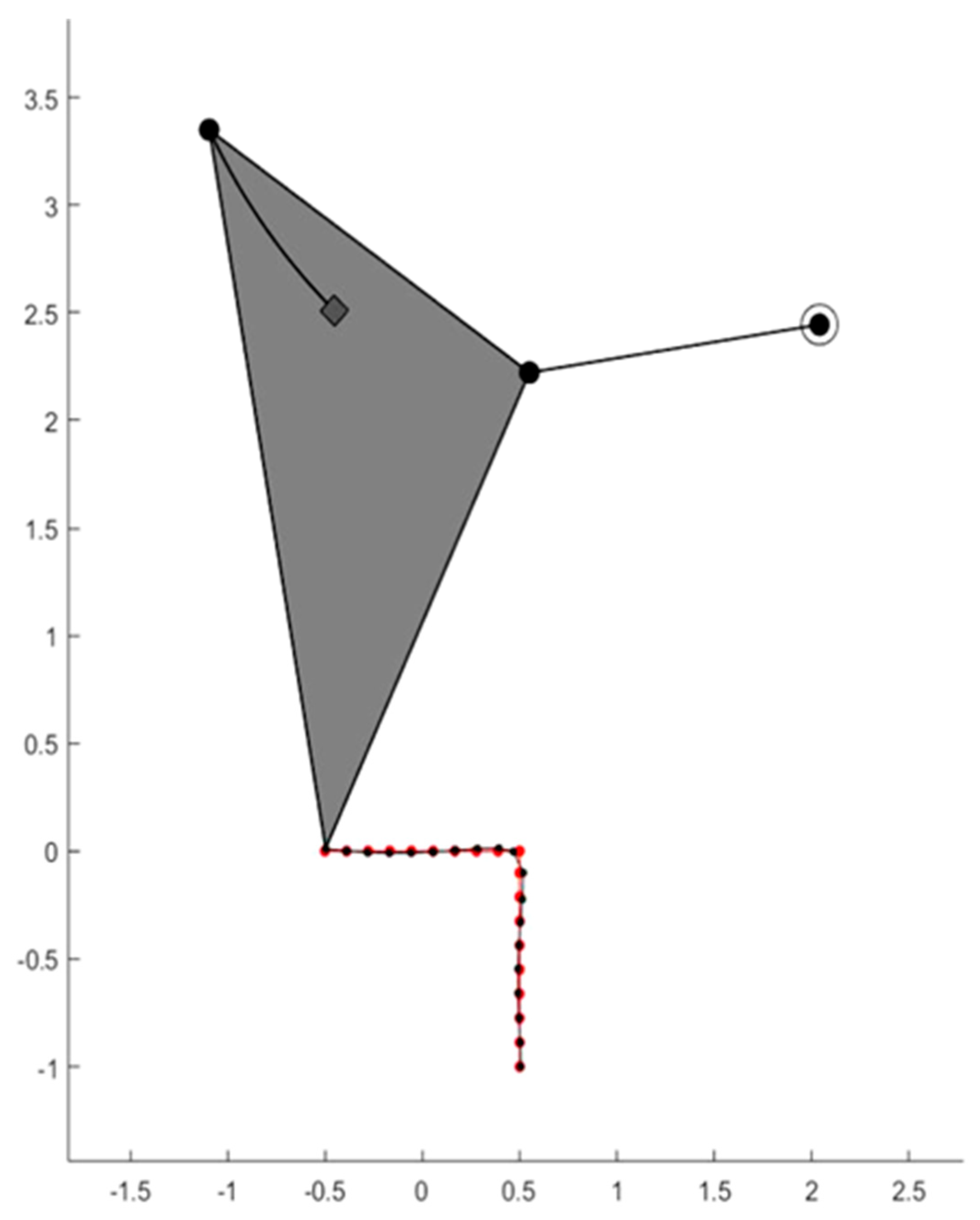
In PG-Example2, the desired trajectory consists of tracing a right angle, as shown in Figure 16 and Figure 17. The data according to the prescribed points are shown in Table 4.
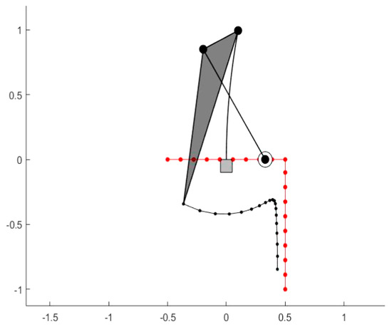
Figure 16.
PG-Example2. Starting mechanism for path generation, error = 1.7507.

Figure 17.
PG-Example2. Optimal mechanism achieved, error = 0.0026.
Table 4.
Coordinates of prescribed points of the objective path of PG-Example2.
Figure 16 and Figure 17 show, respectively, the initial guess mechanism and the optimal solution obtained. As in the previous example, the desired trajectory is depicted in red color, while the initial trajectory (Figure 16) and the obtained optimal one (Figure 17) are depicted in black.
In this example, the value of the error function falls from 1.7507 to 0.0026 after design optimization.
Table 5 displays the dimensional parameters and input values associated with the initial and optimal solutions.
Table 5.
PG-Example2. Starting mechanism and optimal design parameters and inputs.
For PG-Example2, convergence to a final solution is achieved after 50 iterations, with a total computation time of just 0.45 s.
4. Discussion
This work presents a comprehensive study of the coupler curves of a hybrid rigid–flexible four-bar hinged mechanism. Analogies and differences have been established with respect to the well-known rigid four-bar hinged linkage coupler curves. The most notable differences between the hybrid and rigid mechanisms are as follows: in hybrid mechanisms, the curves can contain more than two circuits, even up to ten; “open” circuits can appear; and there cannot be closed circuits with only one branch.
From a classical optimizer based on the gradient of the error function, an optimization algorithm has been created, incorporating this new knowledge about the branches and circuits of the coupler curves of the hybrid rigid–flexible mechanism. Thus, the search for the optimal solution is no longer blind, but is guided by a series of “intelligent” assistants emerging from this new knowledge.
The two examples presented with this path-generation dimensional synthesis procedure demonstrate the effectiveness of this new optimization algorithm, which achieves high-quality solutions, given the possibilities offered by this simple mechanism. Moreover, the algorithm ensures mechanisms that are free of circuit and order errors that are typical of this type of synthesis.
Author Contributions
Conceptualization, A.H., A.M., M.U. and O.A.; methodology, A.H., A.M. and M.U.; software, A.M.; validation, A.H., A.M., M.U. and O.A.; formal analysis, A.H. and O.A.; investigation, A.H., A.M., M.U. and O.A.; resources, A.H. and A.M.; data curation, A.H. and A.M.; writing—original draft preparation, A.H. and A.M.; writing—review and editing, M.U. and O.A.; visualization, A.M. and M.U.; supervision, A.H. and M.U.; project administration, A.H., M.U. and O.A.; funding acquisition, A.H., M.U. and O.A. All authors have read and agreed to the published version of the manuscript.
Funding
This research was funded by the Spanish government through the Ministerio de Ciencia e Innovación (Project PID2020-116176GB-I00), financed by MCIN/AEI/10.13039/501100011033, and funded by the Departamento de Educación from the Regional Basque Government through Project IT1480-22.
Data Availability Statement
Not applicable.
Conflicts of Interest
The authors declare no conflict of interest.
References
- Howell, L.L. Compliant Mechanisms; Wiley: Hoboken, NJ, USA, 2001. [Google Scholar]
- Howell, L.L.; Magleby, S.P.; Olsen, B.M. (Eds.) Handbook of Compliant Mechanisms; Wiley: Hoboken, NJ, USA, 2013. [Google Scholar]
- Rao, P.; Peyron, Q.; Lilge, S.; Burgner-Kahrs, J. How to Model Tendon-Driven Continuum Robots and Benchmark Modelling Performance. Front. Robot. AI 2021, 7, 630245. [Google Scholar] [CrossRef] [PubMed]
- Bryson, C.E.; Rucker, D.C. Toward Parallel Continuum Manipulators. In Proceedings of the 2014 IEEE International Conference on Robotics & Automation (ICRA), Hong Kong, China, 31 May–7 June 2014. [Google Scholar] [CrossRef]
- Orekhov, A.L.; Black, C.B.; Till, J.; Chung, S.; Rucker, D.C. Analysis and Validation of a Teleoperated Surgical Parallel Continuum Manipulator. IEEE Robot. Autom. Lett. 2016, 1, 828–835. [Google Scholar] [CrossRef]
- Lilge, S.; Burgner-Kahrs, J. Kinetostatic Modeling of Tendon-Driven Parallel Continuum Robots. IEEE Trans. Robot. 2023, 39, 1563–1579. [Google Scholar] [CrossRef]
- Trivedi, D.; Rahn, C.D.; Kier, W.M.; Walker, I.D. Soft robotics: Biological Inspiration, State of the Art, and Future Research. Appl. Bionics Biomech. 2008, 5, 99–117. [Google Scholar] [CrossRef]
- Rucker, D.C.; Jones, B.A.; Webster, R.J., III. A Geometrically Exact Model for Externally Loaded Concentric-Tube Continuum Robots. IEEE Trans. Robot. 2010, 26, 769–780. [Google Scholar] [CrossRef]
- Burgner-Kahrs, J.; Rucker, D.C.; Choset, H. Continuum Robots for Medical Applications: A Survey. IEEE Trans. Robot. 2015, 31, 1261–1280. [Google Scholar] [CrossRef]
- Gravagne, I.A.; Rahn, C.D.; Walker, I.D. Large Deflection Dynamics and Control for Planar Continuum Robots. IEEE/ASME Trans. Mechatron. 2003, 8, 299–307. [Google Scholar] [CrossRef]
- Hirose, S.; Yamada, H. Snake-like robots [Tutorial]. IEEE Robot. Autom. Mag. 2009, 16, 88–98. [Google Scholar] [CrossRef]
- Chirikjian, G.S. Theory and Applications of Hyper Redundant Robotics Manipulators. Ph.D. Thesis, California Institute of Technology, Pasadena, CA, USA, 1992. [Google Scholar]
- Chirikjian, G.S.; Burdick, J.W. A modal approach to hyper-redundant manipulator kinematics. IEEE Trans. Robot. Autom. 1994, 10, 343–354. [Google Scholar] [CrossRef]
- Sears, P.; Dupont, P. A Steerable Needle Technology Using Curved Concentric Tubes. In Proceedings of the 2006 IEEE/RSJ International Conference on Intelligent Robots and Systems, Beijing, China, 9–15 October 2006. [Google Scholar] [CrossRef]
- Hannan, M.W.; Walker, I.D. Kinematics and the Implementation of an Elephant’s Trunk Manipulator and Other Continuum Style Robots. J. Robot. Syst. 2003, 20, 45–63. [Google Scholar] [CrossRef]
- Webster, R.J., III; Jones, B.A. Design and Kinematic Modeling of Constant Curvature Continuum Robots: A Review. Int. J. Robot. Res. 2010, 29, 1661–1683. [Google Scholar] [CrossRef]
- Rahn, C. Design of continuous backbone, cable- driven robots. J. Mech. Des. 2002, 124, 265–271. [Google Scholar] [CrossRef]
- Till, J.; Rucker, D.C. Elastic Stability of Cosserat Rods and Parallel Continuum Robots. IEEE Trans. Robot. 2017, 33, 718–733. [Google Scholar] [CrossRef]
- Altuzarra, O.; Solanillas, D.M.; Amezua, E.; Petuya, V. Path Analysis for Hybrid Rigid–Flexible Mechanisms. Mathematics 2021, 9, 1869. [Google Scholar] [CrossRef]
- Altuzarra, O.; Urizar, M.; Cichella, M.; Petuya, V. Kinematic Analysis of three degrees of freedom planar parallel continuum mechanisms. Mech. Mach. Theory 2023, 185, 105311. [Google Scholar] [CrossRef]
- Mauzé, B.; Dahmouche, R.; Laurent, G.J.; André, A.N.; Rougeot, P.; Sandoz, P.; Clévy, C. Nanometer Precision with a Planar Parallel Continuum Robot. IEEE Robot. Autom. Lett. 2020, 5, 3806–3813. [Google Scholar] [CrossRef]
- Hopkins, J.B.; Rivera, J.; Kim, C.; Krishnan, G. Synthesis and Analysis of Soft Parallel Robots Comprised of Active Constraints. J. Mech. Robot. 2015, 7, 011002. [Google Scholar] [CrossRef]
- Singh, I.; Lakhal, O.; Merzouki, R. Towards extending forward kinematic models on hyperredundant manipulator to cooperative bionic arms. J. Phys. Conf. Ser. 2017, 783, 012056. [Google Scholar] [CrossRef]
- Lilge, S.; Nuelle, K.; Boettcher, G.; Spindeldreier, S.; Burgner-Kahrs, J. Tendon Actuated Continuous Structures in Planar Parallel Robots: A Kinematic Analysis. J. Mech. Robot. 2021, 13, 011025. [Google Scholar] [CrossRef]
- Hopkins, J.B.; Culpepper, M.L. Synthesis of multi-degree of freedom, parallel flexure system concepts via freedom and constraint topology (FACT)—Part I: Principles. Precis. Eng. 2010, 34, 259–270. [Google Scholar] [CrossRef]
- Hopkins, J.B.; Culpepper, M.L. Synthesis of multi-degree of Freedom, Parallel Flexure System Concepts via Freedom and Constraint Topology (FACT)—Part II: Practice. Precis. Eng. 2010, 34, 271–278. [Google Scholar] [CrossRef]
- Frecker, M.; Ananthasuresh, G.K.; Nishiwaki, S.; Kikuchi, N.; Kota, S. Topological Synthesis of Compliant Mechanisms Using Multi-Criteria Optimization. J. Mech. Des. 1997, 119, 238–245. [Google Scholar] [CrossRef]
- Mattson, C.A.; Howell, L.L.; Magleby, S.P. Development of Commercially Viable Compliant Mechanisms Using the Pseudo-Rigid Body Model: Case Studies of Parallel Mechanisms. J. Intell. Mater. Syst. Struct. 2004, 15, 195–202. [Google Scholar] [CrossRef]
- Cappelleri, D.J.; Krishnan, G.; Kim, C.J.; Kumar, V.; Kota, S. Toward the Design of a Decoupled, Two-Dimensional, Vision-Based μN Force Sensor. J. Mech. Robot. 2010, 2, 021010. [Google Scholar] [CrossRef]
- Lee, W.T.; Russell, K. Developments in quantitative dimensional synthesis (1970–Present): Four-bar path and function generation. Inverse Probl. Sci. Eng. 2018, 26, 1280–1304. [Google Scholar] [CrossRef]
- Laribi, M.A.; Mlika, A.; Rhomdane, L.; Zeghloul, S. A Combined Genetic Algorithm–Fuzzy Logic Method (GA–FL) in Mechanisms Synthesis. Mech. Mach. Theory 2004, 39, 717–735. [Google Scholar] [CrossRef]
- Kim, J.W.; Jeong, S.M.; Seo, T.W. Numerical Hybrid Taguchi-Random Coordinate Search Algorithm for Path Synthesis. Mech. Mach. Theory 2016, 102, 203–216. [Google Scholar] [CrossRef]
- Mariappan, J.; Krishnamurty, S. A Generalized Exact Gradient Method for Mechanism Synthesis. Mech. Mach. Theory 1996, 31, 413–421. [Google Scholar] [CrossRef]
- Muñoyerro, A.; Hernández, A.; Urízar, M.; Altuzarra, O. A General Automatic Method for Mechanism Optimization Based on Kinematic Constraints and Analytical Jacobian Matrix. Proc. Inst. Mech. Eng. Part C J. Mech. Eng. Sci. 2023, 237, 3181–3197. [Google Scholar] [CrossRef]
- Hernández, A.; Muñoyerro, A.; Urízar, M.; Amezua, E. Comprehensive Approach for the Dimensional Synthesis of a Four-Bar Linkage Based on Path Assessment and Reformulating the Error Function. Mech. Mach. Theory 2021, 156, 104126. [Google Scholar] [CrossRef]
- Ma, O.; Angeles, J. Performance Evaluation of Path-Generating Planar, Spherical and Spatial Four-Bar Linkages. Mech. Mach. Theory 1988, 23, 257–268. [Google Scholar] [CrossRef]
- de Bustos, I.F.; Urkullu, G.; Marina, V.G.; Ansola, R. Optimization of Planar Mechanisms by Using a Minimum Distance Function. Mech. Mach. Theory 2019, 138, 149–168. [Google Scholar] [CrossRef]


Disclaimer/Publisher’s Note: The statements, opinions and data contained in all publications are solely those of the individual author(s) and contributor(s) and not of MDPI and/or the editor(s). MDPI and/or the editor(s) disclaim responsibility for any injury to people or property resulting from any ideas, methods, instructions or products referred to in the content. |
© 2023 by the authors. Licensee MDPI, Basel, Switzerland. This article is an open access article distributed under the terms and conditions of the Creative Commons Attribution (CC BY) license (https://creativecommons.org/licenses/by/4.0/).