Abstract
We present a mathematical model based on ordinary differential equations to investigate the spatially homogeneous state of tumor growth under virotherapy. The model emphasizes the interaction among the tumor cells, the oncolytic viruses, and the host immune system that generates both innate and adaptive immune responses. We conduct a rigorous equilibrium analysis and derive threshold conditions that determine the growth or decay of the tumor under various scenarios. Numerical simulation results verify our analytical predictions and provide additional insight into the tumor growth dynamics.
MSC:
92C50; 37N25
1. Introduction
Tumor virotherapy is a relatively new, yet propitious, strategy in treating cancer [1]. It has shown promising results in preclinical tests and clinical trials for a number of tumor types [2,3,4,5]. This therapy makes use of genetically engineered oncolytic viruses that are specific to tumors. Once injected into a tumor, the viruses infect cancer cells, while leaving healthy cells and tissues unharmed. Through the lysis of the infected cells, the viruses replicate and spread within the tumor and continue infecting other cancer cells. There are several distinct advantages of using virotherapy. First, the replication of oncolytic viruses is highly tumor-selective, and, thus, is generally non-pathogenic to normal tissues. Second, the success rate of viral infection is typically high, as viruses can utilize multiple genetic means to attack tumor cells and cause cell lysis. Moreover, viruses can be genetically manipulated to include additional features so as to achieve improved safety and efficacy [6].
A complication involved in the tumor oncolysis process is the response from the host immune system. Once the viruses start attacking tumor cells, the innate immune response is stimulated by the viruses and the infected tumor cells, which tends to limit virus replication and spread, as well as eliminate infected cells. This anti-virus effect of innate immunity has been well observed and documented [7,8,9]. Recent clinical studies, however, revealed that through the lysis of infected cells, an inflammatory response is induced with the presentation of tumor antigens, which leads to T-cell mediated adaptive immunity against the tumor [6,10]. Thus, the interaction of oncolytic viruses and the immune system contributes to the therapeutic efficacy in two opposite ways: a negative contribution through the anti-virus innate immune response, and a positive contribution through the anti-tumor adaptive immune response.
Ideally, the virotherapy aims to completely remove the tumor cells and the viruses; in the end, though, it is unclear whether such a perfect outcome is realistic. Meanwhile, challenges remain on how to effectively combine the oncolysis and the virus-mediated immunity to ensure the success of the treatment, and how to strategically manipulate the balance between anti-virus and anti-tumor immune responses to achieve the best outcome [1,6,10]. Theoretical investigations and quantitative analysis, particularly using mathematical modeling, can improve our understanding of tumor virotherapy and provide useful guidelines for clinical studies toward overcoming these challenges.
A number of mathematical models have been published on the study of virotherapy and its impact on tumor growth. Wodarz [11] proposed a model based on ordinary differential equations (ODEs), with two compartments representing the infected and uninfected tumor cell populations where each cell population is assumed to grow in a logistic fashion. The model does not explicitly consider viral dynamics, and a main focus of the work is to explore conditions required for maximum reduction of the tumor load. This model was later extended to a more general formulation [12], and two distinct types of dynamics (representing the success and failure of the treatment, respectively) were found, depending on the spread rate of the viruses. Karev et al. [13] employed a similar modeling framework, but with an emphasis on tumor cell heterogeneity. Novozilov et al. [14] incorporated a ratio-dependent functional response into the model of Wodarz [11], and discussed several possible outcomes of oncolytic virus infection, including no effect on the tumor, stabilization or reduction of the tumor load, and complete elimination of the tumor. Tian [15] analyzed the interaction among the infected tumor cells, uninfected tumor cells, and viruses, also using an ODE model, with a focus on the bifurcation study of the virus replicability measured by the burst size. Wang et al. [16] added a nutrient compartment to a model that includes normal cells, tumor cells, and viruses, and explicitly determined the minimum viral dosage in order for the treatment to be effective. None of these ODE models, however, considered the effects of immune responses and their contribution to the efficacy of the therapy.
Meanwhile, virotherapy models based on partial differential equations (PDEs) have also been used. For example, Wu et al. [17] employed a PDE model to compare the evolution of a tumor under different initial conditions that resulted from three virus-injection strategies. This model was later extended in [18] to incorporate a cytokine-based immune response against the virus-infected tumor cells. In addition, Friedma et al. [19] proposed a reaction-convection-diffusion system to investigate tumor virotherapy in the presence of host innate immune response. Although the PDE models in [18,19] both added a separate equation to represent the effects of the host immune response, they only included the innate immunity and did not consider the adaptive immunity, leading to an incomplete picture for the host immune system dynamics in the course of tumor virotherapy. In a more recent study, Timalsina et al. [20] proposed a PDE modeling framework for tumor virotherapy that incorporates both the innate and adaptive immune responses in the description of the interaction among tumor cells, oncolytic viruses, and host immune systems. Due to the complexity of their PDE system, however, the study in [20] was primarily focused on numerical simulation under a variety of parameter settings, and no mathematical analysis was conducted.
The present paper aims to improve our knowledge of the tumor growth dynamics under virotherapy and the tumor–virus–immunity interaction involved in this process, through a rigorous analysis of an ODE model closely related to the PDE model proposed in [20]. Specifically, we are interested in better understanding the spatially homogeneous state of tumor growth, where theory of differential equations and dynamical systems [21,22] can be applied and a detailed equilibrium analysis can be conducted. The simplified ODE model retains all the variables and the essential temporal dynamical features from the original PDE system. Particularly, it remains as a moving boundary problem where the tumor size changes with time, and the innate and adaptive immune responses are both included. Using this ODE model, we will carefully investigate the complex interaction among tumor cells, oncolytic viruses, and innate and adaptive host immune systems, and derive threshold conditions to quantify the success and failure of the virotherapy.
The remainder of this paper proceeds as follows. In Section 2, we describe our ODE model that depicts the spatially homogeneous state in the course of tumor growth under virotherapy. In Section 3, we analyze the equilibria of the model and their stability properties, as well as their impact on the growth of the tumor. We present some numerical simulation results in Section 4, and conclude the paper with some discussion in Section 5.
2. Model Formulation
As a starting point, we first present the PDE model proposed in [20] that describes the interaction between the tumor cells, oncolytic viruses, and innate and adaptive host immune responses. This model, formulated as a moving boundary problem, considers a spherical tumor with radial symmetry and consists of the following equations
for and , where t denotes the time and denotes the spatial distance measured from the center of the tumor. The variables , and are the numbers of normal (i.e., not yet infected), infected, and dead tumor cells, respectively; and are the numbers of the innate and adaptive immune cells, respectively; is the number of viruses, and denotes the moving boundary of the tumor. The motion of all the cells is modeled as a convection process along the radial direction with a velocity , whereas the motion of the viruses (which are much smaller than cells) is modeled as a diffusion process. Since the total cell density is approximately a constant ( cells/mm) [19], with a normalization procedure, it can be assumed that
i.e., each of these variables represents a portion of the total density. In addition, all the parameters involved in this model are described in Table 1.

Table 1.
Model parameters.
We will focus on the spatially homogeneous state of tumor growth. To that end, we assume
That is, all the cells and viruses are uniformly distributed over the spatial domain so that each of these density variables only depends on time. Meanwhile, we retain the spatiotemporal dependence of the convective velocity field:
However, we remark that if we assume a spatially uniform velocity field , it would lead to a stationary tumor with a fixed boundary (i.e., ), which is much easier to analyze but is unrealistic in some sense. A detailed discussion of that scenario is provided in the Appendix A. The spatiotemporal variation of U defined in Equation (4) allows us to study a more realistic and complex tumor with a moving boundary.
With these assumptions, we can manipulate the convection terms in system (1). For example, from the first equation of system (1) we have
where
Equation (6) is obtained by adding up the first five equations in system (1) and using the condition (2). Meanwhile, since , we have
i.e., the diffusion term in the virus equation vanishes. In addition, Equation (5) yields
Integrating both sides for yields
Thus, we obtain the following ODE system
Note that we have dropped the equation for N in the system above. Substituting the expression of f from Equation (6), we may rewrite the first five equations in system (8) as follows:
Meanwhile, the last equation in system (8) yields
In what follows, we will focus our attention on the analysis of the equlibria of system (9); each equilibrium represents a steady state in the tumor virotherapy, where the tumor would grow or decay at a constant rate. Ideally, we would hope that the virotherapy can eliminate all the uninfected tumor cells (i.e., X) to ensure a successful outcome. Practically, however, the uninfected tumor cells may or may not be eradicated, yet the tumor could still be effectively controlled in the presence of some level of uninfected tumor cells [19,20]. Thus, in this study we measure the success of the tumor virotherapy by the (exponential) decay of the tumor radius, whose motion is described by Equation (10), at a stable equilibrium. On the other hand, when an equilibrium is unstable, that implies such a steady state cannot be sustained, or may not be reached at all.
3. Equilibrium Analysis
Let the unknowns of system (9) be ordered as . Each density variable is non-negative to be biologically meaningful. To facilitate our analysis, we introduce the notations
We also assume that , and . These assumptions are consistent with the published parameter values in the literature (see, e.g., [18,19]).
3.1. Trivial Equilibria
It is straightforward to observe that there are four simple boundary equilibria (or, trivial equilibria):
By computing the Jacobian matrices associated with these points, we obtain their characteristic polynomials
respectively. Let us define the threshold value of system (9) by
The threshold value , which is analogous to the basic reproductive number in an infectious disease model, quantifies the capability that the oncolytic viruses can effectively invade the tumor. Specifically, Equation (12) expresses the threshold value as a ratio of two factors which have opposite effects on the outcome of the virotherapy: the ‘positive-effect’ factor represented by the product of the viral reproduction rate and infection rate, and the ‘negative-effect’ factor represented by the virus removal rate and tumor cell reproduction rate.
We then obtain that the equilibrium is locally asymptotically stable if and unstable if . Biologically, the point represents a steady state indicating a complete ‘failure’ of the tumor virotherapy; i.e., uninfected tumor cells occupy of the domain while all other cells and viruses are gone. Our observation here is that when the viral infection/invasion capability is low (such that ), the virotherapy would most likely fail. In that scenario, we have at the stable equilibrium , so that the tumor radius would exponentially grow at a constant rate based on Equation (10). On the other hand, as long as the threshold value is higher than unity, becomes unstable which implies that such a state (of complete treatment failure) would not be attained. Meanwhile, the other three equilibria , and are always unstable as their characteristic polynomials each has at least one positive root. Each of these three points represents an ‘ideal’ steady state of the tumor treatment which is free of tumor cells and viruses. Our results show that the tumor growth cannot stabilize at these equilibria regardless of the value of the threshold value, implying that, practically, such a perfect treatment outcome may not be achieved.
3.2. Immunity-Free Equilibria
In addition to these four simple equilibria, system (9) possesses a number of equilibrium points which are more complex in nature. We proceed to first analyze those equilibria that are free of immune cells, i.e., . We will distinguish two cases, depending on the values of the lysis rate of the infected tumor cells () and the removal rate of the dead tumor cells ().
Case 1:.
It is easy to find that there exists a biologically feasible, immunity-free, equilibrium
if and only if . The Jacobian matrix at is
where , . Hence, the characteristic polynomial of is
with
Let , then and , . Hence,
Consider the following function
One can easily verify that and , hence . In addition, since
there exists a such that for and for . Hence, if we let , then for and for . Thus, by Routh–Hurwitz stability criterion, each root of has a negative real part if and only if and . Moreover, is equivalent to
Hence, it is easy to obtain that , where
Therefore, we conclude that is locally asymptotically stable if and unstable if . At the point , direct calculation yields
Hence, the tumor radius will be exponentially increasing if , and decreasing if .
The immunity-free equilibrium represents a steady state where uninfected tumor cells, infected tumor cells, and viruses co-exist, but both innate and adaptive immune cells vanish. In particular, the density of the infected tumor cells is positive at , indicating some degree of success for the viral invasion into the tumor. Effective control of the tumor, however, depends on the stability of and the value of at that steady state. Consequently, the threshold value has to be in a certain range, i.e., , to ensure a successful outcome of the tumor virotherapy.
Case 2:.
One can verify that the immunity-free equilibrium exists if and only if . Furthermore, and thus , which implies . Hence, is locally asymptotically stable if and thereby the tumor radius would decrease if .
When , there is an additional immunity-free equilibrium in the form of
and , , and are all eigenvalues of the Jacobian at . Note that
Hence, is locally asymptotically stable if . This additional equilibrium represents a success of the tumor virotherapy, where only the infected tumor cells and viruses co-exist while the uninfected tumor cells and immune cells all vanish. At , it is straightforward to obtain , i.e., the tumor radius would exponentially decrease to 0.
3.3. Single-Immunity Equilibria
Next, we explore the equilibria of system (9) where one of the immune components ( and ) may be nonzero. If and , we can solve the following equations
Since , then has a unique positive solution
In addition, , since , and
Hence, there exists a unique innate-immunity-free equilibrium
if and only if .
Similarly, if and , then
Solve X and Y as functions of ,
Let
One can verify that , , and thereby
Since , then has a unique soultion if ; i.e.,
Thus, if , system (8) has a unique adaptive-immunity-free equilibrium
Each of the two equilibrium points and represents a tumor steady state where uninfected tumor cells, infected tumor cells, viruses, and one type (either innate or adaptive) of immune cells co-exist. Through direct calculation, we find at , for . Hence, the tumor would grow if and decay if at the state ().
3.4. Dual-Immunity Equilibria
Lastly, if both immune components are nonzero at an equilibrium, , then . Hence, there exists an equilibrium such that only if ; i.e.,
Let
Then we can show that only two equilibrium points can possibly exist under this setting: one which is free of uninfected tumor cells when , and the other whose components are all positive (an interior equilibrium) when . We discuss these two cases separately as follows.
Case (i):.
Through some algebraic manipulation, one can obtain that the first such equilibrium must take the form
The equilibrium exists if and only if
This equilibrium represents another steady state of successful tumor virotherapy, where all normal (i.e., uninfected) tumor cells are eliminated. In fact, at we can easily calculate , which indicates that the tumor radius would exponentially decrease toward 0.
Case (ii):.
On the other hand, to find the interior equilibrium, we solve the following equations
and obtain
Let , then the interior equilibrium is determined by the root of . Note that is an increasing function, hence, there is a unique root if and only if ; i.e.,
and
These yield
where
For the existence of an interior equilibrium in the form of
with all positive components, it clearly only requires ; i.e., based on Equation (36). Since , the following condition
is sufficient to ensure the existence of where all the tumor cells (uninfected and infected), immune cells, and viruses co-exist and balance each other. If is stable, the success of the tumor treatment at this steady state also depends on the value of defined in Equation (27): the tumor grows if and decays if .
4. Numerical Results
We now conduct numerical simulation to verify our analytical results presented in Section 3. Meanwhile, since the stabilities of several equilibria (such as , , and ) are challenging to analyze mathematically, our numerical findings will provide useful insight into the system dynamics near these equilibrium points.
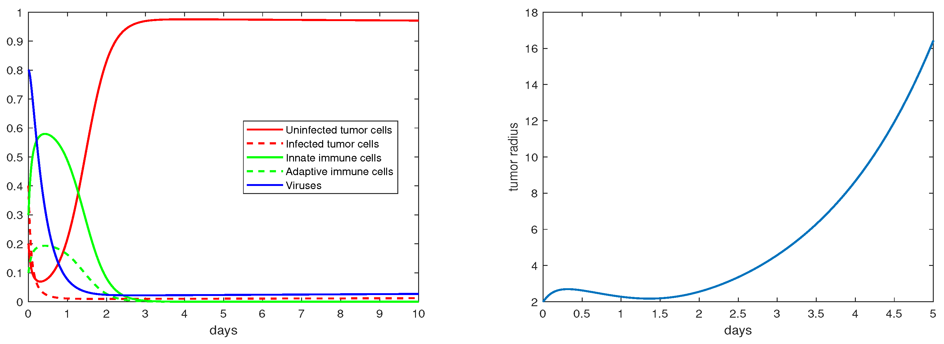
The definition and units of all the model parameters are listed in Table 1. We first conduct a numerical simulation using a set of baseline values for these parameters from the literature [19,20], where such parameters have been fitted to experimental data. The simulation results are presented in Figure 1, with the left panel showing the evolution of the density variables and the right panels showing the evolution of the tumor radius R. The parameter values are given in the caption. We observe that shortly after the start of the therapy (i.e., ), the tumor radius stops growing and even decreases slightly, indicating that the virotherapy is taking effect. This period lasts about 1.5–2 days, after which the oncolytic virus loses its effectiveness and the tumor starts to grow exponentially. Correspondingly, the density of the uninfected tumor cells first decreases, and then increases to and stabilizes at a level close to , while the density of the viruses decreases to a level near 0 after about 1.5 days. This pattern of tumor evolution is qualitatively consistent with the experimental observations [8,20].

Figure 1.
Simulation results for the base scenario. The values of the the parameters are: , .
Next, we vary some of these parameters within their biologically feasible ranges to explore the rich dynamics of tumor growth under different settings that represent a range of possible treatment scenarios. For each figure set presented below, the left panel shows the time evolution of the density variables and the right panel depicts the change of the tumor radius with respect to time. The parameter values are specified for each set of results (see the caption of each figure).
Regarding the trivial equilibria studied in Section 3.1, Figure 2 demonstrates that is locally asymptotically stable when . In particular, note that the percentage of the uninfected tumor cells (X) is at this steady state. Correspondingly, the tumor radius is exponentially increasing (in a hypothetic way) with a constant rate once the tumor growth stabilizes at the equilibrium .
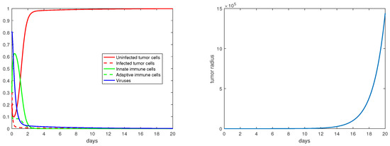
Figure 2.
The equilibrium is asymptotically stable and the tumor radius is exponentially increasing when . The values of the the parameters are: , , , , .
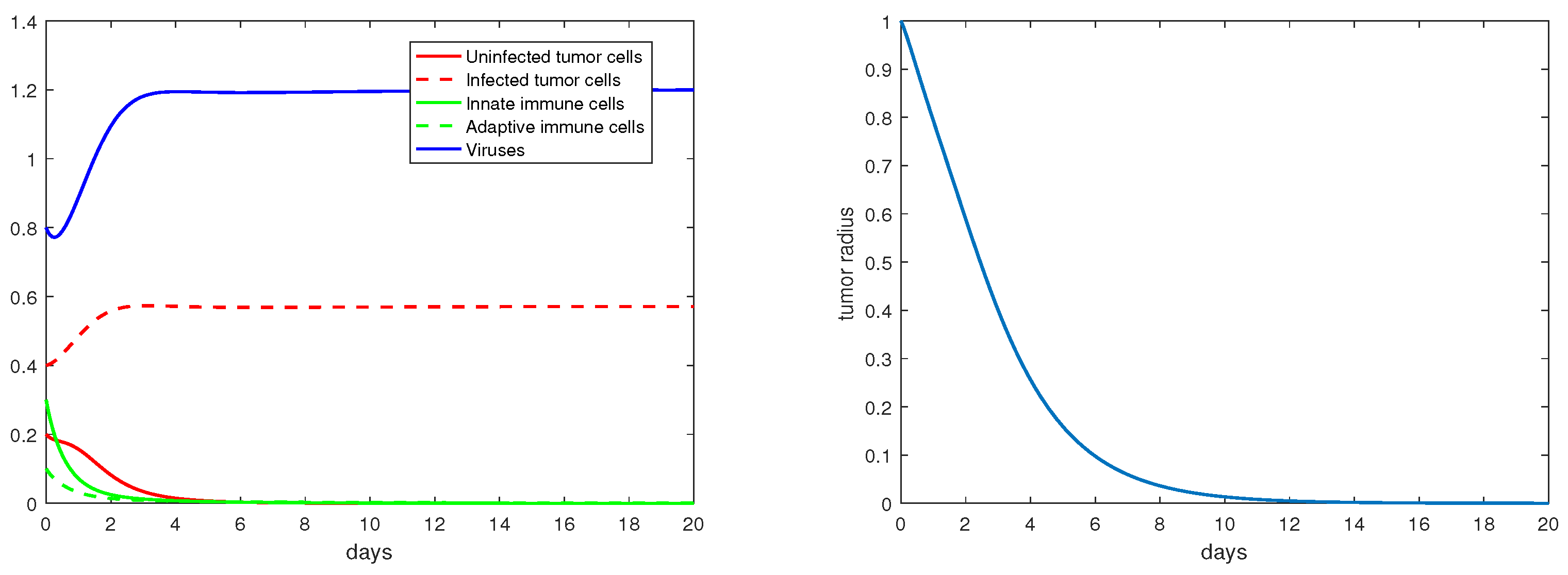
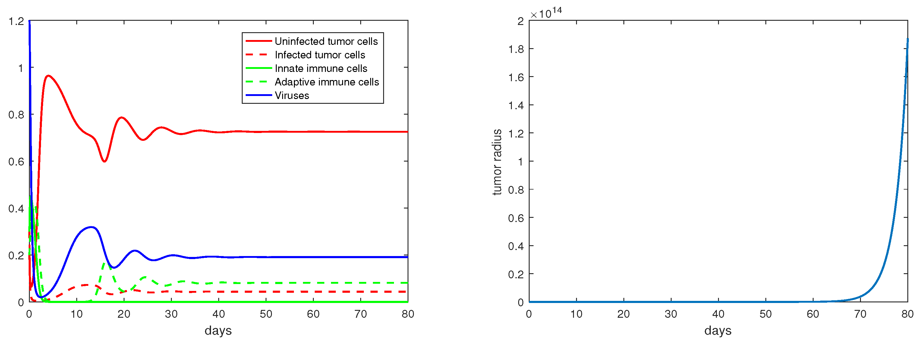
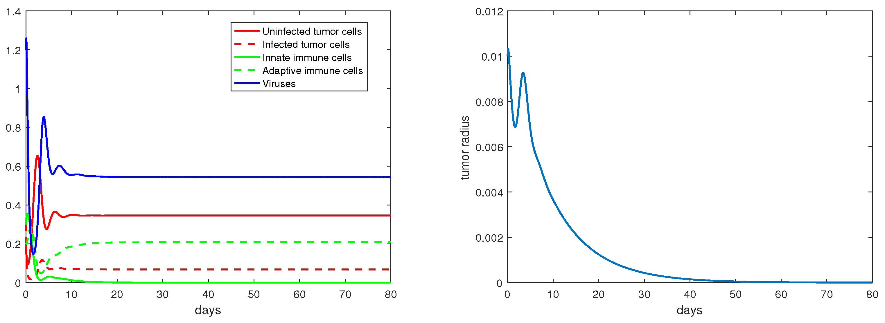
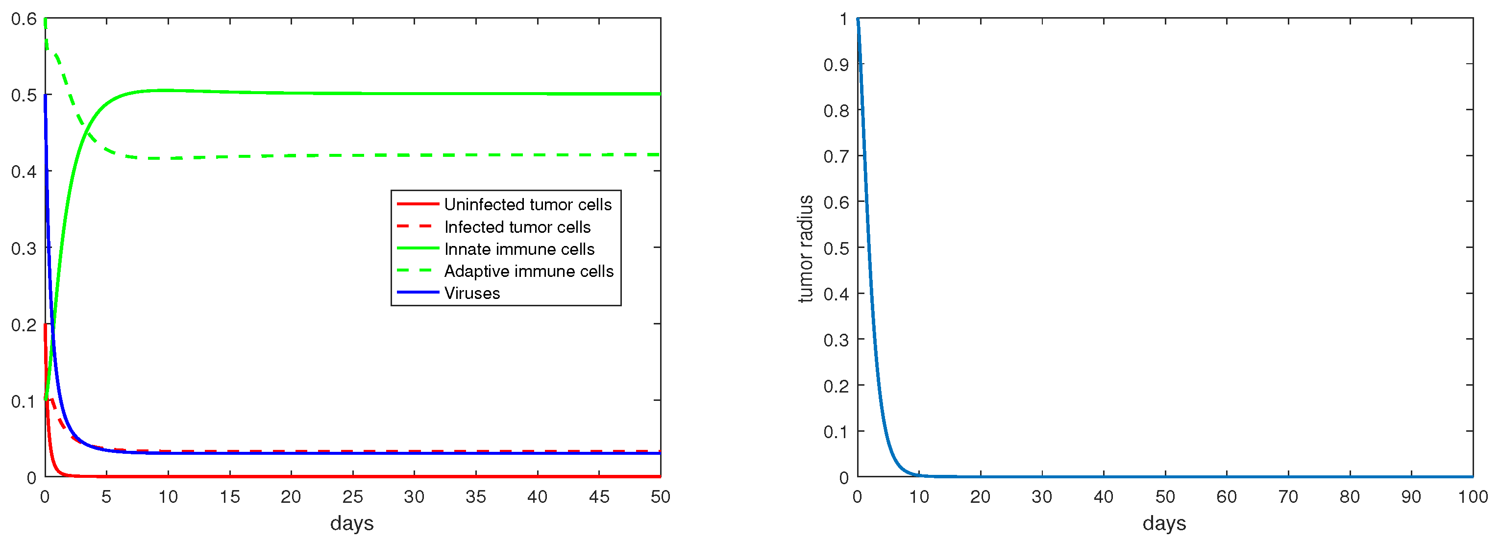
For the immunity-free equilibria, Figure 3, Figure 4, Figure 5 and Figure 6 provide numerical verification of the analytical predictions in Section 3.2. Figure 3 and Figure 4 show that is locally asymptotically stable when and . At this stable equilibrium, the tumor would grow if ; this is illustrated in Figure 3 where . On the other hand, the tumor would decay if , as illustrated in Figure 4 where . Figure 5 and Figure 6 illustrate the dynamics associated with and when . Figure 5 shows that is locally asymptotically stable and the tumor radius decreases to 0 when . Note also that the percentage of the uninfected tumor cells is pretty low () at this steady state. Figure 6 shows that is locally asymptotically stable when , and in this case, , thereby the tumor radius is exponentially decreasing to 0.
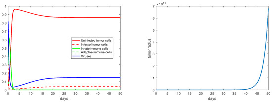
Figure 3.
The equilibrium is asymptotically stable and the tumor radius is exponentially increasing when and . The values of the parameters are: , , , , .

Figure 4.
The equilibrium is asymptotically stable and the tumor radius is exponentially decreasing when and . The values of the parameters are: , , , , .
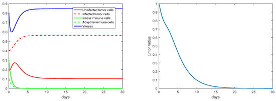
Figure 5.
The equilibrium is asymptotically stable and the tumor radius is exponentially decreasing when and . The values of the parameters are: , , , , .
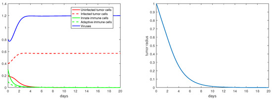
Figure 6.
The equilibrium is asymptotically stable and the tumor radius is exponentially decreasing when and . The values of the parameters are: , , , , .
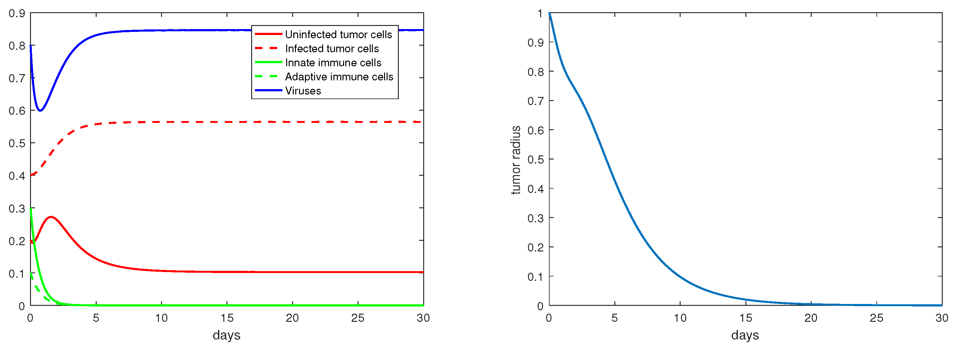
Concerning the single-immunity equilibria analyzed in Section 3.3, Figure 7 and Figure 8 depict the local stabilities of and , respectively. At the equilibrium point , the tumor growth rate is determined by for . With the parameter setting in Figure 7, , and with that in Figure 8, . Thus, the tumor radius is exponentially increasing in each case. We note that the levels of the uninfected tumor cells remain very high (more than ) for both steady states. In contrast, Figure 9 shows that at the equilibrium the tumor radius is decreasing to 0, where and where the uninfected tumor cells are only about .
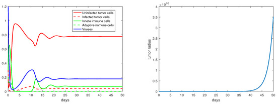
Figure 7.
The equilibrium is asymptotically stable and the tumor radius is exponentially increasing when . The values of the parameters are: , , , , .
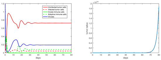
Figure 8.
The equilibrium is asymptotically stable and the tumor radius is exponentially increasing when . The values of the parameters are: , , , , .
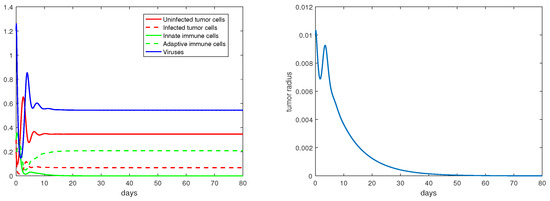
Figure 9.
The equilibrium is asymptotically stable and the tumor radius is exponentially decreasing when . The values of the parameters are: , , , , .
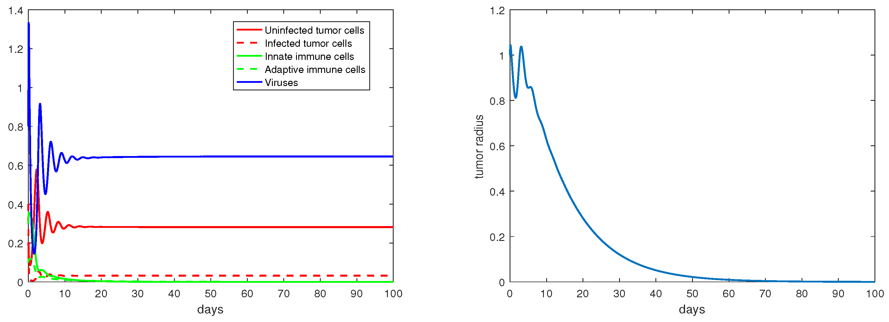
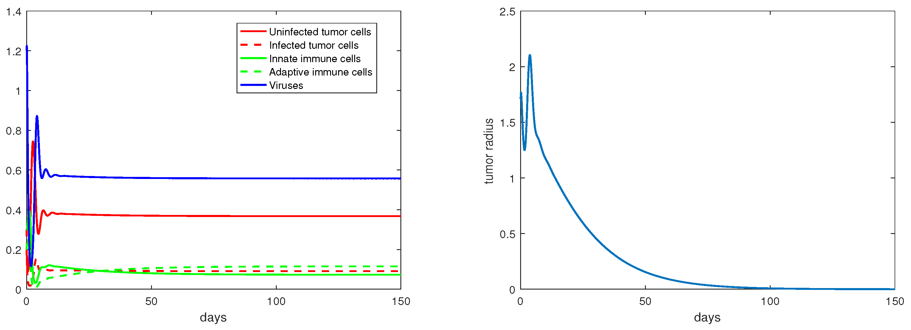
Regarding the dual-immunity equilibria investigated in Section 3.4, Figure 10 illustrates that when the equilibrium exists and is stable, the tumor radius at that state will decay and approach 0, where . In addition, if there is a stable interior equilibrium , then the tumor radius at would also be decreasing to 0 if . This is verified in Figure 11, where .
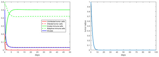
Figure 10.
The equilibrium is asymptotically stable and the tumor radius is exponentially decreasing when . The values of the parameters are: , , , , .

Figure 11.
The equilibrium is asymptotically stable and the tumor radius is exponentially decreasing when . The values of the parameters are: , , , , .
5. Discussion
We have presented an ODE model to describe the spatially homogeneous state of tumor growth under virotherapy. This model, derived and simplified from the PDE system (1), enables us to conduct a detailed analysis on the time evolution of the tumor radius and the various equilibrium points, their stability properties, and their impact on tumor growth.
Our model describes the process of tumor growth as a moving boundary problem. The threshold value introduced in our analysis represents the capability that the oncolytic viruses can effectively invade the tumor. When , for example, the stability of the equilibrium and the exponential increase of the tumor radius at indicate a failure of the tumor treatment due to the insufficient invasion capability of the viruses. Consequently, provides a necessary condition for effective viral invasion, though the eventual outcome of the tumor therapy would be determined by the specific dynamical properties at an equilibrium and the associated tumor growth rate. When is above unity, both the number of the equilibrium points and the complexity of the dynamics increase. In general, each equilibrium represents a steady state, and the tumor growth dynamics near such a steady state are shaped by the interaction among the uninfected and infected tumor cells, the innate and adaptive immune cells, and the viruses. Although the dynamical behaviors for some of the equilibria (, , and ) have not been fully resolved analytically, our numerical simulation results provide helpful insight into their stability and connection to the growth rate of the tumor.
Our results show that the threshold value can be used to as an indicator regarding the chance of success for tumor virotherapy. The value of can be modified by genetically manipulating the viruses; for example, increasing the burst size b (which leads to a larger ) is an effective strategy to improve the efficacy of the virotherapy [19]. From the modeling perspective, the higher is, the better outcome the therapy might achieve. From the practical point of view, however, it is not possible to increase in an arbitrary manner. Meanwhile, high value of might come at the price of some side effects of the tumor treatment, such as harming normal body tissues surrounding the tumor [19]. Our analysis and simulation results show that the virotherapy can achieve a success for relatively low (for example, between 1 and 2), as long as we can push the solution orbit into the basin of attraction for one of those stable equilibrium points where the associated tumor growth rate is negative. These findings could provide useful guidelines for the design of practical virotherapy protocols to improve the rate of success for tumor treatment.
It is known that some tumors (such as melanoma, kidney cancer, and lung cancer) are likely to trigger a strong adaptive immune response and are commonly referred to as “hot tumors”, while some other tumors (such as glioblastoma, prostate cancer, and breast cancer) are able to suppress the adaptive immune response and are commonly referred to as “cold tumors”. Our model could offer useful insight into the treatment of these two types of tumors. In particular, the parameter in our model measures the rate of fighting cancerous cells due to the adaptive immune response. Our results suggests that an increased value of could improve the performance of the tumor therapy, as shown in Figure 10 and Figure 11 where the tumor radius quickly decays and approaches 0. This parameter represents the T-cell infiltration rate in practical tumor treatment. In fact, many therapeutic strategies have been proposed to increase the T-cell infiltration rate so as to possibly turn a cold tumor into a hot tumor [23].
Our model can be naturally extended to include other approaches for tumor treatment, such as chemotherapy and radiation therapy. The combination of these different treatment options could potentially achieve a better performance than using a single therapy, and the mathematical model could help to quantify and predict the treatment outcome. In addition, the current model does not take into account potential mutations of the oncolytic viruses. This could be an interesting direction for our future modeling effort.
Tumor growth is a highly complex process that involves rich temporal and spatial dynamics. This paper is focused on the temporal growth dynamics of the tumor and related equilibrium analysis, without considering the spatial heterogeneity. It may be important to mathematically investigate the spatial heterogeneity of tumor growth in some situations, and a few quantitative studies have been performed in this direction (see, e.g., [24,25]). These models are generally simpler than the PDE model (1), though their analytical tools might be generalized to handle more complex tumor models such as (1).
Author Contributions
Conceptualization, J.W.; Methodology, C.Y. and J.W.; Formal analysis, C.Y.; Investigation, C.Y. and J.W.; Writing—original draft, C.Y. and J.W.; Writing—review & editing, J.W. All authors have read and agreed to the published version of the manuscript.
Funding
This research was partially funded by the National Science Foundation grant numbers 1951345 and 1913180.
Data Availability Statement
Not applicable.
Conflicts of Interest
The authors declare no conflict of interest.
Appendix A. Homogeneous State with a Fixed Boundary
With the assumption in (3), if we additionally assume that the velocity field is spatially uniform; i.e., , then we have
This yields and . Consequently, we obtain , and the tumor would be stationary with a fixed boundary under this setting.
As a result, we obtain the following ODE system
To simplify the notation, let us define
Clearly, the system (A1) has a trivial equilibrium and an immunity-free equilibrium . Based on their Jacobian matrices
their characteristic polynomials are
respectively. Hence, and are both unstable since is a positive eigenvalue for , and the polynomial has at least one root with positive real part based on the Routh–Hurwitz criterion. In addition, leads to the equilibrium
and leads to the equilibrium
Their associated characteristic polynomials can be written as follows
where , () are constants determined by the parameters in model (A1). One can verify that and . Hence, and are both unstable by the Routh–Hurwitz criterion.
Our analysis of this scenario, which represents a spatially homogeneous tumor state with a fixed boundary, shows that all the equilibrium points are unstable. This result implies that a tumor cannot stabilize under such a setting; instead, the tumor size has to change with time in the presence of tumor–virus–immune interaction, leading to the more realistic (and more complex) scenario with a moving tumor boundary.
References
- Shah, A.C.; Benos, D.; Gillespie, G.Y.; Markert, J.M. Oncolytic viruses: Clinical applications as vectors for the treatment of malignant gliomas. J. Neurooncol. 2003, 65, 203–226. [Google Scholar] [CrossRef] [PubMed]
- Kasuya, H.; Takeda, S.; Nomoto, S.; Nakao, A. The potential of oncolytic virus therapy for pancreatic cancer. Cancer Gene Ther. 2005, 12, 725–736. [Google Scholar] [CrossRef] [PubMed]
- Kirn, D.H.; McCormick, F. Replicating viruses as selective cancer therapeutics. Mol. Med. Today 1996, 2, 519–527. [Google Scholar] [CrossRef] [PubMed]
- Kirn, D.; Hermiston, T.; McCormick, F. ONYX-015: Clinical data are encouraging. Nat. Med. 1998, 4, 1341–1342. [Google Scholar] [CrossRef]
- Parato, K.A.; Senger, D.; Forsyth, P.A.; Bell, J.C. Recent progress in the battle between oncolytic viruses and tumours. Nat. Rev. Cancer 2005, 5, 965–976. [Google Scholar] [CrossRef] [PubMed]
- Chiocca, E.A.; Rabkin, S.D. Oncolytic viruses and their application to cancer immunotherapy. Cancer Immunol. Res. 2014, 2, 295–300. [Google Scholar] [CrossRef]
- Lawler, S.E.; Chiocca, E.A. Oncolytic virus-mediated immunotherapy: A combinatorial approach for cancer treatment. J. Clin. Oncol. 2015, 33, 2812–2814. [Google Scholar] [CrossRef]
- Fulci, G.; Breymann, L.; Gianni, D.; Kurozomi, K.; Rhee, S.S.; Yu, J.; Kaur, B.; Louis, D.N.; Weissleder, E.; Caligiuri, M.A.; et al. Cyclophosphamide enhances glioma virotherapy by inhibiting innate immune responses. Proc. Natl. Acad. Sci. USA 2006, 103, 12873–12878. [Google Scholar] [CrossRef]
- Wein, L.M.; Wu, J.T.; Kirn, D.H. Validation and analysis of a mathematical model of a replication-competent oncolytic virus for cancer treatment: Implications for virus design and delivery. Cancer Res. 2003, 63, 1317–1324. [Google Scholar]
- Melcher, A.; Parato, K.; Rooney, C.M.; Bell, J.C. Thunder and lightning: Immunotherapy and oncolytic viruses collide. Mol. Ther. 2011, 19, 1008–1016. [Google Scholar] [CrossRef]
- Wodarz, D. Viruses as antitumor weapons: Defining conditions for tumor remission. Cancer Res. 2001, 61, 3501–3507. [Google Scholar]
- Komarova, N.L.; Wodarz, D. ODE models for oncolytic virus dynamics. J. Theor. Biol. 2010, 263, 530–543. [Google Scholar] [CrossRef] [PubMed]
- Karev, G.P.; Novozhilov, A.S.; Koonin, E.V. Mathematical modeling of tumor therapy with oncolytic viruses: Effects of parametric heterogeneity on cell dynamics. Biol. Direct 2006, 1, 30. [Google Scholar] [CrossRef] [PubMed]
- Novozhilov, A.S.; Berezovskaya, F.S.; Koonin, E.V.; Karev, G.P. Mathematical modeling of tumor therapy with oncolytic viruses: Regimes with complete tumor elimination within the framework of deterministic models. Biol. Direct 2006, 1, 6. [Google Scholar] [CrossRef]
- Tian, J.P. The replicability of oncolytic virus: Defining conditions on tumor virotherapy. Math. Biosci. Eng. 2011, 8, 841–860. [Google Scholar] [PubMed]
- Wang, Z.; Guo, Z.; Peng, H. A mathematical model verifying potent oncolytic efficacy of M1 virus. Math. Biosci. 2016, 276, 19–27. [Google Scholar] [CrossRef]
- Wu, J.T.; Byrne, H.M.; Kirn, D.H.; Wein, L.M. Modeling and analysis of a virus that replicates selectively in tumor cells. Bull. Math. Biol. 2001, 63, 731–768. [Google Scholar] [CrossRef]
- Wu, J.T.; Kirn, D.H.; Wein, L.M. Analysis of a three-way race between tumor growth, a replication-competent virus and an immune response. Bull. Math. Biol. 2004, 66, 605–625. [Google Scholar] [CrossRef]
- Friedman, A.; Tian, J.P.; Fulci, G.; Chiocca, E.A.; Wang, J. Glioma virotherapy: Effects of innate immune suppression and increased viral replication capacity. Cancer Res. 2005, 66, 2314–2319. [Google Scholar] [CrossRef]
- Timalsina, A.; Tian, J.P.; Wang, J. Mathematical and computational modeling of tumor virotherapy with mediated immunity. Bull. Math. Biol. 2017, 79, 1736–1758. [Google Scholar] [CrossRef]
- Murray, J.D. Mathematical Biology, 3rd ed.; Springer: Berlin/Heidelberg, Germany, 2007. [Google Scholar]
- Asamoah, J.K.K.; Nyabadza, F.; Jin, Z.; Bonyah, E.; Khan, M.A.; Li, M.Y.; Hayat, T. Backward bifurcation and sensitivity analysis for bacterial meningitis transmission dynamics with a nonlinear recovery rate. Chaos Solitons Fractals 2020, 140, 110237. [Google Scholar] [CrossRef]
- Liu, Y.T.; Sun, Z.J. Turning cold tumors into hot tumors by improving T-cell infiltration. Theranostics 2021, 11, 5365–5386. [Google Scholar] [CrossRef] [PubMed]
- Hinow, P.; Gerlee, P.; McCawley, L.J.; Quaranta, V.; Ciobanu, M.; Wang, S.; Graham, J.M.; Ayati, B.P.; Claridge, J.; Swanson, K.R.; et al. A spatial model of tumor-host interaction: Application of chemotherapy. Math. Biosci. Eng. 2009, 6, 521–546. [Google Scholar] [PubMed]
- Preziosi, L. Cancer Modelling and Simulation; Chapman Hall/CRC Press: Boca Raton, FL, USA, 2003. [Google Scholar]
Disclaimer/Publisher’s Note: The statements, opinions and data contained in all publications are solely those of the individual author(s) and contributor(s) and not of MDPI and/or the editor(s). MDPI and/or the editor(s) disclaim responsibility for any injury to people or property resulting from any ideas, methods, instructions or products referred to in the content. |
© 2023 by the authors. Licensee MDPI, Basel, Switzerland. This article is an open access article distributed under the terms and conditions of the Creative Commons Attribution (CC BY) license (https://creativecommons.org/licenses/by/4.0/).

