3.1. Bernstein Representation
Bernstein polynomials [
26] of degree
n on interval
are defined as
Then, each function
,
and
can be linearly represented as
where
are some constants that are not all zero, and this equation can also be written as
where
is called the Bernstein representation vector of function
on
.
On the support interval of
, consistent with the previous settings, the number of elements in
is
. For each n,
stands for the whole set of Bernstein polynomials:
Then
and the corresponding representation matrix is
where
Compared with the representation matrix in [
19], matrix
represents functions in
at each recursive level
n.
Definition 3 ( function). A function defined over , and is called a function if it is at most continuous at breakpoints within its support interval.
functions are not equivalent to functions in a
MD-spline basis, a
MD-spline basis only requires continuity at the join of different degrees. For example, a
MD-spline basis may contain B-splines; however, B-splines are not
continuous at their internal breakpoints. A
MD-spline basis has some particular properties, such as the integrals of functions in it can be computed easily, which is used in [
20].
functions are also particularly to be used in this section, as their Bernstein presentation vectors are easily expressed.
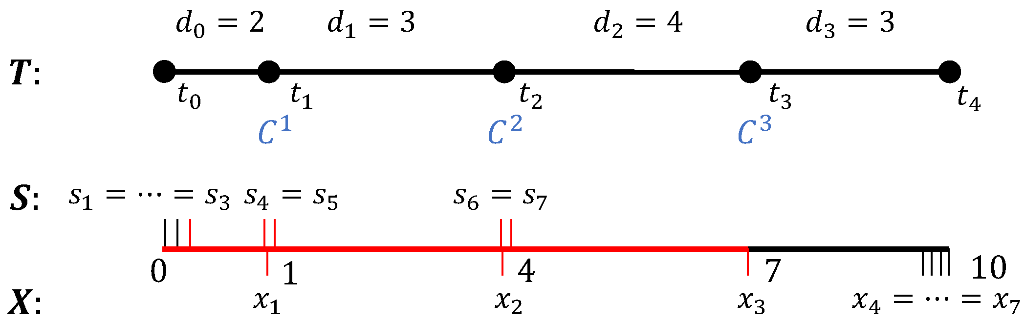
Example 1. Consider a MD-spline basis with , and . The first function and the last function are Bernstein polynomials. Function is continuous at , and it is plotted in red in Figure 2. Other functions are all B-spline functions, where are functions and are functions. In addition, all functions define a MD-spline basis. It holds is a function, and its Bernstein representation vector on each interval is composed of an entry equal to 1 and the rest are equal to 0, while the Bernstein representation vectors of B-spline functions include several nonzero entries.
3.2. Recursive Process
The recursion of Bernstein representation vectors is determined by Equation (
6) and the integral property of Bernstein polynomial [
26]. Each vector
is affected not only by
, but also by
and
; hence, the recursive relationship should be evaluated on distinct intervals.
On interval
, consider the following
matrix
The integral of Bernstein polynomials satisfy the equality
According to the integral formula, the integral of
is determined as follows:
Similarly, another part of the integral is
The integral recursion can be substituted by the recursive process of Bernstein representation vectors according to Equation (
19). The matrix
H is just presented in (
18) for simplicity of expression. A cumulative-sum operation can be used to describe the recursion of a representation vector in calculation.
Without loss of generality, assuming that
on interval
, it holds that
We indicates the cumulative-sum operation by an operator
:
Then, we use an operator
to extract the last element of a vector. For example,
. Then,
Consider
. The integral starting from
is
where
is a constant, and
is a vector. The symbol ⊕ means that
is added to each element in
.
Using the two operators above,
can be calculated as follows:
Consistent with the conventional B-splines, functions in an MD-spline basis can be independently calculated using a recursive method. According to the Bernstein representation, once the vector is calculated, function is determined. Consequently, Bernstein representation vectors can replace functions in the recursive process.
The support interval of , is ; therefore, there are intervals in it. Therefore, we establish an initial matrix ; each entry is 0 and indicates a vector .
Matrix has rows, which means that there are corresponding functions on when . However, the indexes of these functions may exceed the limit range . There are two solutions for this. One does not generate rows whose indexes surpass the maximum allowed range. The other one disregards these rows because all of their elements equal 0. In order to make the algorithm more understandable, we employ the second solution. In the recursive process, we use these vectors to explain the recursion of matrix in the algorithm.
There are some details in this procedure.
The operation (line 12) causes vectors with the same index j have the same length, hence allowing these vectors can bulid the matrix .
(line 15) indicates the row of the matrix , and . Thus each row is normalized.
There are only two cases of subtraction without considering the subtraction of zero rows (line 19 and 21).
The subtraction is performed in range (lines 20, 22 and 23).
Algorithm 1 only calculates one function in MD-spline basis. If vectors in the initial matrix are changed to be , all basis functions are produced.
The following is an example for Algorithm 1.
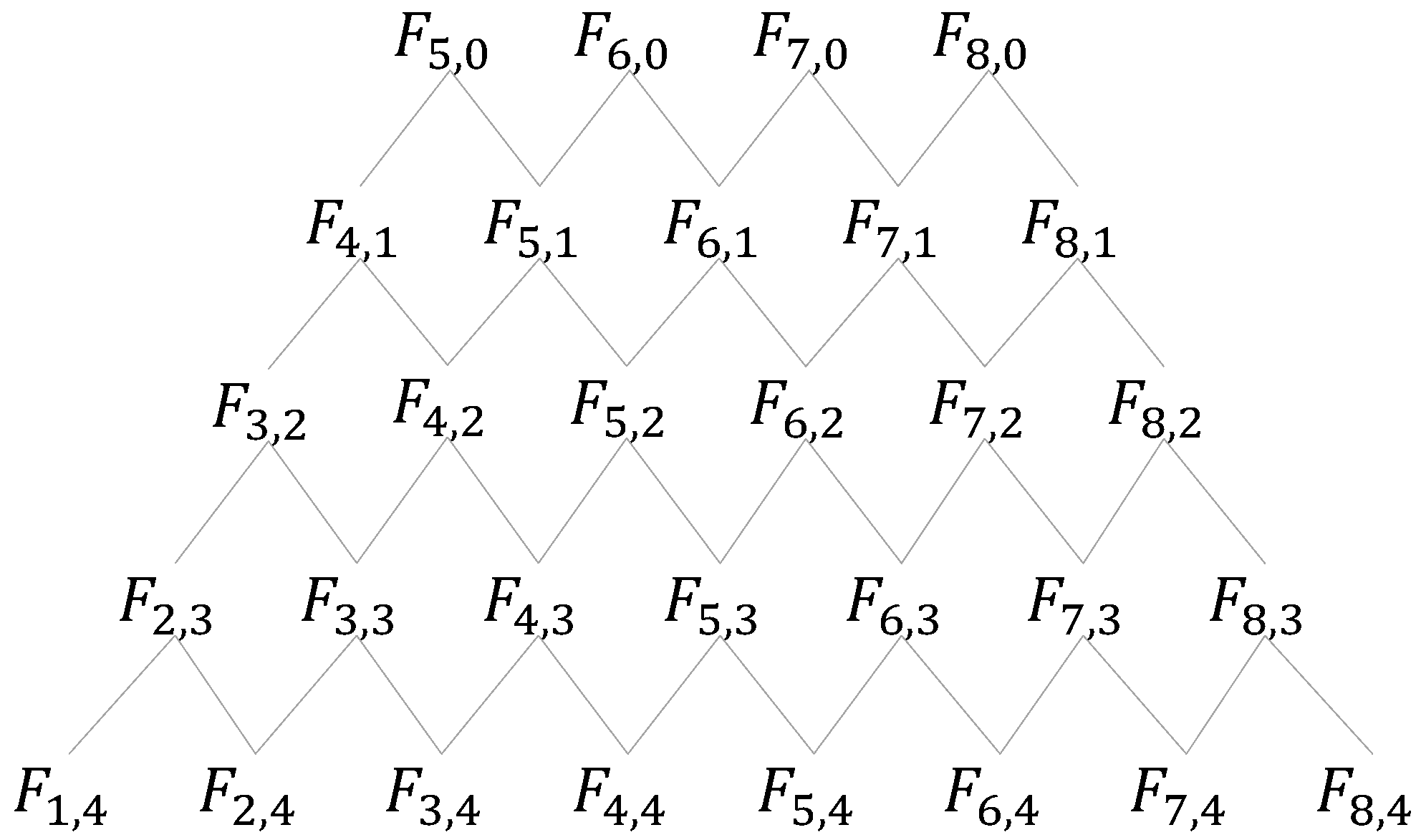
Example 2. Consider a MD-spline basis with , , and . Two extended partition are and . We are aming to calculate function . These partitions are shown in Figure 3. The support interval of is , and . Thus the order of the initial matrix is , then At the beginning of each loop, value 1 is assigned to the vector that satisfies the condition in line 5 in Algorithm 1. Therefore, .
| Algorithm 1 Recursive process of Bernstein representation vectors. |
Input:, , , i
Output:- 1:
Initial , ; - 2:
for n to do - 3:
for k to do - 4:
for j to do - 5:
ifthen - 6:
end if - 7:
end for - 8:
for j to do - 9:
- 10:
end for - 11:
for j ← to do - 12:
if () and () then - 13:
end if - 14:
end for - 15:
ifthen - 16:
end if - 17:
end for - 18:
for k to do - 19:
if and then - 20:
- 21:
else if and then - 22:
- 23:
- 24:
end if - 25:
end for - 26:
Delete the last row of ; - 27:
end for
|
Because there is no function when . In order to be concise, we start the calculation from . In this case, it is easy to get : In the third row of M, the results of cumulative sum and normalization operations are as follows:and Thus . Note that . After normalization, this row changes into Similarly, the second row changes into According to the substraction in Algorithm 1, equals to on interval and on interval . After substraction can be computed in the same manner. Then, remove the third row and change into the subsequent one: By repeating these operations, then the final vector will be This example can aid comprehension of this section. Although only a portion of the calculation is displayed, the entire recursion is similar. The representation matrix may be calculated directly, and this method is quite intuitive and straightforward to comprehend.
3.3. Algorithm Analysis
The numerical stability of Algorithm 1 is influenced by the floating point operations. There are three types of operations in the algorithm.
- 1
Cumulative sum operation: the operation in Algorithm 1 (line 9) is composed of addition and multiplication. All elements in the vector are positive and increasing. If the length of an interval is excessively long, the number of bits of elements may vary significantly. This procedure frequently executes this operation, resulting in numerical inaccuracies.
- 2
Normalized operation: this operation restricts all elements in to the range . Since the denominator is the largest number in this vector and all members are positive, this operation will not result in a significant amount of numerical inaccuracy.
- 3
Subtraction operation: Equation (
19) prevents the scenario where two approximate floating point-numbers are subtracted.
The complexity of Algorithm 1 depends on the settings of the sequences
, so, like reference [
20], we only count the number of operations.
At each recursive level in Algorithm 1, there are no more than non-zero rows of each . Therefore, the total number of non-zero rows will not exceed in the whole recursive process.
Cumulative sum operation: the number of elements in is ; thus, the number of this operation will not exceed .
Normalized operation: each non-zero row will be normalized, so the maximum number of this operation is .
Subtraction operation: similarly, there are subtraction operations, at most.
Thus, the number of operations will not exceed , which is used to estimate the numerical complexity of Algorithm 1.
Due to the recursive nature of Algorithm 1, the cyclical calculation of floating-point numbers may lead to error accumulation. Based on the preceding research, the cumulative sum operation is the primary source of mistake. This error can be reduced by a bidirectional algorithm, and Equation (
6) is reformed as follows:
where . The symbol means rounding down operation.
Then, Algorithm 1 is modified, and the subsequent Algorithm 2 is more numerically stable in calculation.
To represent the reverse integral, we define two reverse operators. Consistent with the prior setting
, then
and
. Algorithm 2 is as follows:
| Algorithm 2 Revised recursive method. |
- 1:
Same setting as Algorithm 1; - 2:
for n to do - 3:
for k to do - 4:
for j to do - 5:
if then - 6:
end if - 7:
end for - 8:
end for - 9:
; - 10:
for j to do - 11:
; - 12:
; - 13:
end for - 14:
Extend zero vectors; - 15:
if then - 16:
end if - 17:
if then - 18:
end if - 19:
for k to do - 20:
for j to do - 21:
; - 22:
end for - 23:
for j to do - 24:
; - 25:
end for - 26:
for j← to do - 27:
; - 28:
end for - 29:
for j to do - 30:
- 31:
end for - 32:
end for - 33:
Delete the last row of ; - 34:
end for
|
3.4. Numerical Experiment
In [
20], three typical methods for calculating an MD-spline basis are compared, which are named RKI/Greville, RKI/Derivative and H-Operator. Due to the higher order derivative operations, RKI/Derivative and H-Operator are not numerically stable, while RKI/ Greville avoids these operations and it is numerically stable.
Then, we will design some experiments in
Table 1 to test Algorithms
1 and
2. Calculation results are divided into ’Exact’ and ’Numerical’. The ’Exact’ results rely on the symbolic computation in MATLAB, while the ’Numerical’ results are determined by the standard precision in MATLAB (rounding unit
).
Example 3. Values in Table 2 are calculated from Algorithm 1, where ’Exact’ in the second column indicates that the Bernstein representation matrix is calculated through symbolic computation. Exact MD-spline basis and Bernstein basis are also calculated by symbolic computation. The absence of relative error in the third column demonstrates that Algorithm 1 is correct. Example 4. This experiment demonstrates that Algorithm 1 requires revision. The addition of two floating integers with significantly dissimilar digits will result in significant numerical errors. In Table 3, the value produced by Algorithm 1 on the third row has a large relative error and does not symmetric with the first value, whereas the problem is avoided by Algorithm 2. Example 5. Table 4 illustrates the values and relative errors of for Test 3. The RKI/Greville method is unquestionably stable. Algorithm 2 has adequate numerical precision in this instance, where the highest degree exceeds 20. This algorithm is typically stable in experiments below this degree. Example 6. This experiment shows that the efficiency of different methods, as measured by MATLAB execution time. Results in Table 4 are calculated using the same point values for four tests. All tests are performed on an environment consisting of MATLAB 2020a and the AMD Ryzen 5 4600U. Calculating the values of basis functions at the internal knots yields the running time. Note that Algorithm 2 can calculate a single function in the MD-spline basis; its experiment is divided into two separate instances. The information displayed in the second column of Table 4 represents the duration of a single basis function. In order to ensure that values of this function are not zero at most knots, we select the middle basis function. A second scenario involves calculating the values of all basis functions at knots. Based on the data in Table 5, it is evident that the efficacy of Algorithm 2 is assured. When the degree of basis is low, as in Test 1 and Test 2, there is little difference between the computation times of single functions and whole functions. However, as the degree increases, so does the efficiency gap. In some extreme cases, such as Test 4, the degrees of the basis functions are extremely high, making it inefficient to calculate the values of all functions. As the RKI/Greville method is calculated on separate pieces, it needs longer running time.
Compared to the RKI/Greville method, Algorithm 2 is less accurate numerically but more efficient in its calculations. Using a B-spline basis instead of a Bernstein basis as representation functions can improve the numerical precision due to the smaller representation matrix reducing the number of floating-point operations.
Recursive Bernstein representation is not only meaningful for calculation, but it also provides a tool for investigating the recursive relations of MD-spline.


