Article

Effect of Learning and Forgetting on Inventory Model under Carbon Emission and Agile Manufacturing

1
Department of Mathematics, Inderprastha Engineering College, Ghaziabad 201010, India
2
Department of Mathematics, Chaudhary Charan Singh University, Meerut 250001, India
3
Department of Industrial and Management Engineering, Pohang University of Science and Technology, 77, Cheongam-ro, Nam-gu, Pohang-si 37673, Republic of Korea
4
Department of Industrial Engineering, Yonsei University, 50 Yonsei-ro, Sinchon-dong, Seodaemun-gu, Seoul 03722, Republic of Korea
5
Center for Transdisciplinary Research (CFTR), Saveetha Dental College, Saveetha Institute of Medical and Technical Sciences, Saveetha University, 162, Poonamallee High Road, Velappanchavadi, Chennai 600077, India
*
Author to whom correspondence should be addressed.
Mathematics 2023, 11(2), 368; https://doi.org/10.3390/math11020368
Submission received: 11 November 2022 / Revised: 25 December 2022 / Accepted: 5 January 2023 / Published: 10 January 2023

Abstract

:
The aim of this study is to examine the learning and forgetting effect on a manufacturer’s production process with volume agility and carbon emission costs. During COVID-19, the learning rate becomes very low, and the forgetting rate becomes very high. That is why, the analysis of the learning and forgetting effects on the production process is very important. This research finds an effect of learning and forgetting on the manufacturer and on reducing the unit manufacturing cost. Here, the production rate is a function of the number of units produced, and it is taken as a decision variable through agile manufacturing. Here, the Weibull deterioration rate is used, and the production process is subject to the learn–forget–learn policy. Here, a carbon emission cost is introduced into the setup/ordering cost, holding cost, and item cost for the manufacturer. The effect of learning and forgetting is analyzed through numerical examples.

1. Introduction

The necessity of learning and forgetting is related to human beings and is concerned with any business. The study is conducted on a production model to test the effectiveness of learning and forgetting. A common behavior of human beings is forgetting after this learning, as the capacity of the human brain is not the same. Thus, the rate of learning and forgetting is not the same, too. As human labor is involved within the production system, hence, depending on the rate of a specific laborer’s learning and forgetting, the profile of a company may vary. If the learning rates of laborers are more and the forgetting rates are lower, then the company will always benefit from the gathered knowledge of the laborers, but if the opposite is true, then the company may have to invest a high amount to train the laborers repeatedly to maintain the business. Therefore, a study of the effectiveness of learning and forgetting is really important for the production section. However, based on the learning, the production rate may vary from any fixed rate to a variable production rate, specifically an increasing rate. Thus, there is a need to study an agile production system rather than a basic traditional production system. This study is conducted on the agile production of any production with deterioration and the effect of carbon emissions during production.
The rest of the paper is oriented as follows: Section 2 explains the literature review; Section 3 shows the assumptions and notation. The formulation of a mathematical model for a manufacturer is provided in Section 4. Numerical verifications, with sensitivity analysis, are provided in Section 5. Section 6 presents the important observations examined through numerical verifications. The conclusions and further research are shown in Section 7.

2. Literature Review

This section contains a discussion of several studies related to this study from the literature.

2.1. Flexibility in Manufacturing System

Any manufacturing system aims to produce items continuously at a fixed rate and ensure that all items are of good quality. With a constant production rate, the average cost of production is reduced, but during slumps in demand, there is a need to store the stock produced. Therefore, the holding cost increases. On the other hand, if the rate of production is taken as a decision variable, then the cost of production decreases, and hence the holding cost decreases. Through a system of agile manufacturing, the controllable production rate can be easily used such that the production rate increases or decreases based on the necessity of management. The production rate varies depending on the situation. Manufacturing companies mostly have flexible manufacturing systems (FMSs) to improve production efficiency. Khouja [1] analyzed a production model with imperfect production and a flexible production rate [2]. On the other hand, a model was developed on a volume-flexible, stock-dependent inventory model [3]. A supply chain model with flexible manufacturing was formulated, with the holding cost taken as a variable [4]. Again, Singh et al. [5] developed an economic order quantity (EOQ) model, with the demand rate taken as a variable, along with volume agility and inflation. A volume-flexible production model under inflation considering trapezoidal demand was developed by Mehrotra et al. [6]. Singhal and Singh [7] developed an inventory model with multivariate demand under volume flexibility and learning. Singh and Vandana [8] analyzed a vendor–buyer model having errors in the inspection process and a demand rate that depends on the selling price under volume agility. A viable inventory policy for imperfect production under the effect of energy and volume agility was formulated by Kamna et al. [9]. Recently, Sarkar et al. [10] worked on the reliability of a flexible manufacturing system under supply chain management. They expressed that for a smart manufacturing system with a smart machine and smart technologies, smart labor is essential. Jauhari et al. [11] studied a green production system to reduce emissions using flexibility in the system. Jauhari et al. [12] proposed an adjustable production rate for an imperfect production system. An investment was used to reduce the defective rate.

2.2. Effect of Learning and Forgetting Process

For the good quality of items, the process of learning plays an important role in inventory management. The performance of a system on a repetitive task improving with time is implied as learning. Improvement in the system is found in manufacturing industries in the form of cost and unit production time reduction. If there is a huge time lapse during successive production processes, the production rate may not be as high as it was at the time of stopping production when the production resumes. This leads to an increase in cost and production time with an increase in the period of break. The performance loss during the break is because of forgetting. When learning–forgetting effects on production time and cost are significant, it affects the inventory system as well.
The learning and forgetting phenomenon are as follows:
(a)
Learning phenomenon
The learning phenomenon was introduced by Wright [13]. Wright’s power function is given as
t n = t 1 n r
Here, tn is the production time for the nth unit, t1 is the time required to produce the first unit, n is the production count, and r is the slope of the learning curve, computed as r = −logλ/log 2, where λ is learning rate, and tn = tmin > 0.
(b)
Forgetting phenomenon
The forgetting curve relation (c.f. Carlson and Rowe [14]) is expressed as
t ^ μ = t ^ 1 μ l
where t ^ μ is the equivalent time for the μth unit of lost experience of the forgetting curve, μ is the number of units that would have been produced if interruption did not occur, t ^ 1 is the intercept of the forgetting curve, and l is the slope of the forgetting curve, reflecting an increase in the production time required per unit.
In the literature on inventory models, many papers incorporate the effect of learning and forgetting. This model described learning, lost time, and economic production. Elmaghraby [15] explained economic manufacturing quantities under conditions of learning and forgetting. Jaber and Boney [16] formulated a mathematical model that developed a model on learning–forgetting effects on the optimal lot size of intermittent production. When the system experienced a partial transmission of learning, carrying fewer inventories in later lots was the optimal policy. Jaber and Boney [17] described the economic manufactured/order quantity (EMQ/EOQ) and the learning curve. Jaber and Kher [18] formulated a dual-phase learning–forgetting model (DPLFM). Balkhi [19] explained the learning effects of the optimal production lot size for deteriorating and partially backordered items with time-varying demand and deterioration rates [20]. Jaber and Kher [21] derived a theory on the learn–forget curve model (LFCM) with variant and invariant time to total forgetting. Jaber et al. [22] described lot sizing with learning–forgetting and entropy cost. Das et al. [23] proposed a production inventory model for a deteriorating item incorporating a learning effect using a genetic algorithm. Mahapatra et al. [24] explained a fuzzy production inventory model with shortages and time-dependent learning and forgetting for deteriorating items. Bachar et al. [25] developed a sustainable smart manufacturing model using an outsourcing policy. Kumar and Goswami [26] investigated an EPQ model with learning, partial backlogging, and imperfect production in a fuzzy environment. Kazemi et al. [27] formulated an EOQ model considering backorders and forgetting effects in a fuzzy environment. Ahmad and Chen [28] formulated a model on strategies for short-term energy demand forecasting utilizing machine-learning-based models. Batarfi et al. [29] developed a model for inventory decisions and pricing in a dual-channel supply chain with learning–forgetting. Marchi et al. [30] studied the learning effect on manufacturing companies. Learning by doing improved the quality of products and increased the speed of the production rate. Marchi et al. [31] developed a green supply chain model with a learning effect on a production system.

2.3. Carbon Emissions

Through the help of each member of an organization, a production system can reduce carbon emission costs in an integrated model. Sarkar et al. [32] formulated a model for a multiphase manufacturing system with a random defective rate. Sarkar et al. [33] developed a three-echelon supply chain model with variable transportation and carbon emissions for biodegradable products. Padiyer et al. [34] analyzed a model with a multi-echelon supply chain process for upgrading the quality of items. Habib et al. [35] formulated a supply chain model for the biodiesel supply chain considering carbon emissions. Hota et al. [36] discussed smart technologies to overcome the unreliability of supply chain players. Yadav et al. [37] formulated a model for pollution reduction in supply chain management. Moon et al. [38] developed an economic production model with controlled carbon emissions in the production system. They made a reliable production system with variable setup costs. A dual-channel retailing for substitutable products were derived by Sarkar et al. [39]. They decided to reduce carbon emissions using a carbon tax policy. Wangsa [40] presented a joint economy model for the random demand of buyers. They considered shortages to be partially backordered. To reduce greenhouse gas emissions, they implemented penalty and incentive policies from the government. Marchi et al. [41] proved that the speed of production affects the deterioration of products, machine breakdown, and greenhouse gas emissions. They used vendor-managed inventory with a consignment policy and a classical policy to find the optimum cost for the supply chain. Castellano et al. [42] proposed a heuristic algorithm to minimize greenhouse gas emissions during production and transportation. Daryanto et al. [43] developed a three-echelon supply chain model for deteriorated products. They minimized carbon emissions produced due to transportation and total supply chain cost.
The above researchers assumed learning and forgetting for the manufacturer only and did not incorporate volume agility in their models (Table 1). Very few researchers explained the concept of learning and forgetting with volume agility and carbon emission cost. Therefore, there is a gap in this area. To fill this gap, this paper is formulated by using learning and forgetting in the production model for the manufacturer. In this model, the demand rate is taken as an exponential function of time for the manufacturer. The deterioration rate follows the Weibull distribution for both manufacturers. In this study, a numerical example is shown to analyze the effect of volume agility on the total cost function. Numerous studies have been performed based on the effect of learning and forgetting on the lot size, but the study of learning and forgetting with agile manufacturing and carbon emission cost is a research topic that has not emerged yet. Therefore, there is no investigation into this matter from both theoretical and experimental standpoints. To fill the research gap, a production model is designed for the manufacturer.

3. Problem Description, Notation, and Assumptions

3.1. Problem Description

In this model, a production inventory model is optimized under volume agility, investment of carbon emission cost, and learning and forgetting. Moreover, the production rate is a component of the number of units produced in time t, and the production process is subject to learn-forget-learn (LFL). In this scenario, the deterioration rate depends on environmental conditions. It is analyzed that, during COVID-19, many items deteriorated in shopping malls. Therefore, in this model, the Weibull deterioration rate is used. The manufacturing system of the manufacturer is subjected to exponential demand, and a carbon emission cost is applied.

3.2. Notation

Please see Appendix A for the notation table.

3.3. Assumptions

The items are subject to deterioration with the Weibull distribution function, i.e., δ(t) = αβtβ−1, where α is the scale parameter, β is the shape parameter, and there is no repair or replacement of the deteriorating items.
The demand rate is an exponential function of time for the manufacturer, which is denoted by D(t) = aebt, where a > 0, b > 0, and a > b (see reference [44]).
The increasing production rate (due to learning) for a single item produced in lots is denoted by P(t), where P ( t ) = d Q ( t ) d t , Q(t) is the number of units produced up to time t, and the process of production is subject to LFL (see reference Alamri and Balkhi [20]).
The total forgetting time depends on the number of units remembered.
The cost of production per unit of time depends on the production rate (P) and is given below (Bachar et al. [24]).
φ ( P ) = ( k + g P ( t ) + s P ( t ) )
where k is the material cost, g is the development cost, and sP is associated with tool/die cost and is proportional to the production rate.
Carbon emission cost is introduced into the holding cost, item cost, and setup/ordering cost at the manufacturer’s end.

4. Mathematical Modeling

We develop and describe an inventory model (IM) for a total cost per unit of time. The IM with a manufacturer has projected in a manner that the manufacturer produces items at a production rate P. Here, the production rate is a function of the number of units produced in time t, and the number of units is taken as the decision variable. The demand rate is exponential. Carbon emission cost is included in the ordering/setup, item cost, and holding cost of the items.

4.1. Manufacturer’s Model

Imj(t) denotes the inventory level at time t for cycle j. The system starts operating at time T0j in each cycle j (j = 0,1, 2, …), by which the production process starts, and there is an increase in inventory level due to production and decreases due to demand and deterioration until the inventory level reaches its maximum level and production stops, i.e., time T1j. Now the system undergoes forgetting from time T1j to time T2j. In this period, due to demand and deterioration, the inventory level decreases and becomes zero by time T2j. Figure 1 exhibits the behavior of the inventory level.
The following differential equations give the behavior of the inventory level.
I m j ( t ) = P ( t ) D ( t ) δ ( t )   I m j ( t ) ,   T 0 j t T 1 j
I m j ( t ) = D ( t ) δ ( t )   I m j ( t ) ,   T 1 j t T 2 j
Now, the solutions of the above differential equations are
I m j ( t ) = e ϕ ( t ) T 0 j t { P ( u ) D ( u ) } e ϕ ( u ) d u . T 0 j t T 1 j
and
I m j ( t ) = e ϕ ( t ) t T 2 j D ( u ) e ϕ ( u ) d u .   T 1 j t T 2 j
where
ϕ ( t ) = δ ( t ) d t = α β t β 1 d t = α t β
Let I m j ( t 1 , t 2 ) = t 1 t 2 I m j ( u ) d u , then from Equations (6) and (7), one can have
I m j ( T 0 j , T 1 j ) = T 0 j T 1 j e ϕ ( t ) ( T 0 j t [ P ( u ) D ( u ) ] e ϕ ( u ) d u ) d t = T 0 j T 1 j [ ψ ( T 1 j ) ψ ( u ) ] [ P ( u ) D ( u ) ] e ϕ ( u ) d u
Utilizing Equation (8), one can write
I m j ( T 1 j , T 2 j ) = T 1 j T 2 j e ϕ ( t ) ( t T 2 j D ( u ) e ϕ ( u ) d u ) d t I m j ( T 1 j , T 2 j ) = T 1 j T 2 j [ ψ ( u ) ψ ( T 1 j ) ] D ( u ) e ϕ ( u ) d u
where
ψ ( t ) = e ϕ ( t ) d t = e α t β d t = t α t β + 1 β + 1 + α 2 t 2 β + 1 2 ( 2 β + 1 )
(neglecting the higher powers of α ).
Note that we can set T0j = 0 without loss of generality. The manufacturer holds the material holding cost, setup cost, item cost, and production cost. An explanation of these cost components is described here.

4.1.1. Item Cost (this Cost also Includes the Deterioration Cost)

The manufacturer’s item cost per unit of time, including deterioration cost and cost of carbon emissions, is
I C m = ( c m + c m ) 0 T i j P ( u ) d u

4.1.2. Holding Cost

The manufacturer is holding the inventory. For that, the manufacturer has to pay a holding cost hm per unit per unit of time. However, to maintain the EURO-14, the production industry considers the cost of carbon emissions and the additional investment hꞌm per unit per unit of time for holding the inventory. Hence, under the effect of the environment, the total holding cost is
H C m = ( h m + h m ) { 0 T i j ( ψ ( T 1 j ) ψ ( u ) ) ( P ( u ) D ( u ) ) e ϕ ( u ) d u + T i j T 2 j ( ψ ( u ) ψ ( T 1 j ) ) D ( u ) e ϕ ( u ) d u }

4.1.3. Setup Cost

The manufacturer’s setup cost per setup, considering the cost of carbon emissions under the effect of the environment, is
SCm = (Km+ Kꞌm).

4.1.4. Production Cost

The manufacturer’s production cost consists of many costs such as material cost, development cost, and tool/die cost. Here, material cost, development cost, and tool/die cost contain their values and carbon emissions values together rather than separately shown values.
P C m = 0 T i j ( k + g P ( u ) + s P ( u ) ) d u
The total cost of the inventory system per unit of time during the cycle [0, T2j] contains the item cost, inventory holding cost, setup cost, and production cost given by a function of T1j and T2j, say TCm(T1j, T2j), and is expressed as
T C m ( T 1 j   , T 2 j ) = 1 T 2 j   [ ( c m + c m ) 0 T i j P ( u ) d u + ( K m + K m ) + 0 T i j ( k + g P ( u ) + s P ( u ) ) d u + ( h m + h m ) { 0 T i j ( ψ ( T 1 j ) ψ ( u ) ) ( P ( u ) D ( u ) ) e ϕ ( u ) d u + T i j T 2 j ( ψ ( u ) ψ ( T 1 j ) ) D ( u ) e ϕ ( u ) d u } ]
where ϕ ( u ) is given by Equation (7), and ψ (u) is given by Equation (10).
The goal is to find T1j and T2j, which minimize TCm (T1j, T2j), where the variables T1j and T2j are related to each other through the following relations
0 < T1j < T2j
and
e ϕ ( T i j ) 0 T i j ( P ( u ) D ( u ) ) e ϕ ( u ) d u = e ϕ ( T i j ) T i j T 2 j D ( u ) e ϕ ( u ) d u
Relation (17) ensures that the inventory levels are equal for t = T1j. Therefore, our objective is to solve the following optimization problem.
Minimize TCm (T1j, T2j), given by Equation (15), subject to Equation (16) and h1 = 0, where
H 1 = 0 T i j ( P ( u ) D ( u ) ) e ϕ ( u ) d u T i j T 2 j D ( u ) e ϕ ( u ) d u

4.2. Model Formulation under LFL

From the Alamri and Balkhi [20] model, let ηj denote the number of equivalent units of experience remembered at the start of production run j, with the initial amount ηj = 0. In each production run j (j = 1, 2, …), the system starts production at time T0j, in which learning takes place. Hence, the amount ηj will be increased due to the learning effect up to time T1j, where production ceases, and a maximum level of equivalent units of experience Qj is reached, where Qj is the number of units produced in cycle j. At this time, the forgetting phenomenon starts its influence, and hence, the number of equivalent units of experience Qj will be decreased due to the forgetting influence up to time T2j, by which an equivalent amount ηj+1 is reached (ηj+1Qj), and recommencement of the next production is restarted. The process is repeated. Further, if we denote the time required to produce the first unit in cycle j by t1j, then it is to be noted that when the transmission of learning from cycle to cycle does not occur, ηj = ηj+1 = 0 and t1j = t1j+1 = 0. Moreover, if there is a full transmission of learning from cycle to cycle, then ηj+1 = Qj and t1j ≥ t1j+1. The equality is to allow the possibility that if r > 0 => t1j  0 as Qj .
First, we shall present an approximation form for Equation (1). Let tij be the time required to produce the ith unit in the jth cycle, then we have
tij = t1j ir
Then
t j = k = 1 i t 1 j   k r t 1 j 0 i   k r d k = t 1 j i 1 r 1 r
If Qj amount is produced in the interval [T0j, T1j], then from Equation (20), we have
T 1 j     T 0 j   = t 1 j Q j 1 r 1 r
In addition, if Rj is the amount produced in the interval [T1j, T2j], assuming that there is no interruption in production, then from Equation (20), we have
T 2 j     T 0 j = t 1 j ( Q j + R j ) 1 r 1 r
Next, an approximation form for Equation (2) is presented. Let t μ j ^ be the equivalent time to produce the μ th unit in the jth cycle, then from (2), we have
t μ j ^ = t 1 j ^   μ l j
Recalling the definition of   η j + 1   , the time required to produce the first unit in the next production run j can be found from (19) in terms of   η j + 1   as follows:
t 1 j + 1 = t 1 j ( η j + 1 + 1 ) r
The number of equivalent units of experience is equal to the same amount at the beginning of the forgetting phase, i.e., by time T1j when production ceases, namely, Qj is the amount produced in the interval [T0j, T1j]. This can be obtained by equating Equation (19) for I = Qj and (23) for μ = Qj, yielding
t 1 j Q j r = t 1 j ^   Q j l j
from which we obtain
t 1 j ^ = t 1 j Q j ( r + l j )
Substituting Equation (26) in Equation (23), we obtain
t μ j ^ = t 1 j Q j ( r + l j )   μ l j
The number of equivalent units of experience is equal to the amount η j + 1   by time T2j, when the forgetting phase ceases. By equating Equation (23) for μ = (Qj + Rj) and (19) for i =   η j + 1   , it can be obtained, yielding
t 1 j ^ ( Q j + R j ) l j = t 1 j   η j + 1   r
From this and Equation (26), it follows that
  t 1 j   η j + 1   r = t 1 j Q j ( r + l j ) ( Q j + R j ) l j
from which we obtain
  η j + 1   = [ Q j ( r + l j ) ( Q j + R j ) l j ] 1 / r
Let ψ 1 ( Q j ) = Y j be the corresponding quantity produced during the interval [T1j, t1j], where t1jT1j. It is assumed that no intermittence occurred in production. Then, from Equation (21) we have
t 1 j T 0 j   = t 1 j ( Q j + Y j ) 1 r 1 r
Let the equivalent number of Qj units of experience be totally forgotten at time t1j. The number of equivalent units of experience by time t1j can be obtained by (23) for μ = (Qj + Yj) and (19) for i = 1, yielding
t 1 j ^ ( Q j + Y j ) l j = t 1 j
Substituting Equation (26) in Equation (31), we obtain
Q j ( r + l j ) ( Q j + Y j ) l j = 1
Taking the logarithm of both sides, we obtain
l j = r   log ( Q j ) log ( Q j + Y j ) log ( Q j )
The production rate P(t) when the system is subject to forgetting is equivalently given by
P ( t ) = Number   of   units   remembered   up   to   time   t t
For T0j = 0, Equation (21) implies
T 1 j = t 1 j Q j 1 r 1 r
Let
T 1 j = f 1 j ( Q j )
From Equation (34), we have
Q j = [ T 1 j 1 r t 1 j ] 1 / ( 1 r ) P j = d Q j d t = 1 t 1 j [ T 1 j 1 r t 1 j ] r / ( 1 r )
In addition, from Equation (17), we have
0 T i j P ( u ) e ϕ ( u ) d u = 0 T 2 j D ( u ) e ϕ ( u ) d u [ 1 r t 1 j ] 1 / ( 1 r ) [ T 1 j 1 1 r + α ( T 1 j ) β ( 1 r ) + 1 β ( 1 r ) + 1 ] = a [ T 2 j + b   T 2 j 2 2 + α ( T 2 j ) β + 1 β + 1 ]
  1 a   [ 1 r t 1 j ] 1 / ( 1 r ) [ T 1 j 1 1 r + α ( T 1 j ) β ( 1 r ) + 1 β ( 1 r ) + 1 ] = T 2 j
From Equations (35) and (37), we have
T 2 j = f 2 j   ( Q j )
Thus, on substituting Equations (17), (35), and (38) in Equation (15), the problem is converted to the following unconstrained problem with Q j .
  W ( Q j   ) = 1 f 2 j   [ ( c m + c m ) 0 f i j P ( u ) d u + ( K m + K m ) + ( h m + h m ) { 0 f i j ψ ( u ) ( P ( u ) D ( u ) ) e ϕ ( u ) d u + f i j f 2 j ψ ( u ) D ( u ) e ϕ ( u ) d u } + 0 f i j ( μ + g P ( u ) + s P ( u ) ) d u ]
From Equations (7), (10), (36), and (39), we have
  W ( Q j   ) = 1 f 2 j   [ Q j ( c m + c m + s ) + ( K m + K m ) + ( h m + h m ) t 1 j ( 1 r t 1 j ) r / ( 1 r ) { f 2 j   3 f 1 j   3 3 + α β ( f 2 j   β + 3 f 1 j   β + 3 ) ( β + 1 ) ( β + 3 ) } + μ t 1 j Q j 1 r 1 r + g t 1 j ( 1 2 r ) ( 1 r t 1 j ) ( 2 r ( 1 r ) 1 ) / ( 1 r ) ]
Here, f1j and f2j are functions of Qj given in Equations (34), (35), (37), and (38).

4.3. Solution Methodology

The model is solved by the classical optimization method. The necessary condition for having a minimum Equation (40) is
d W d Q j = w Q j   f 2 j f 2 j , Q j   w f 2 j 2 = 0
where W = w f 2 j and w Q j and f 2 j , Q j are the derivatives of w and f 2 j with respect to Q j .
Note that Equation (41) is equivalent to
w Q j   f 2 j = f 2 j , Q j   w
Taking the first derivative of both sides of Equation (17) with respect to Q j , we have
f 1 j , Q j   P ( f 1 j )   e   E M B E D   ϕ ( f 1 j ) = f 2 j , Q j     D ( f 2 j )   e   E M B E D   ϕ ( f 2 j )
From Equations (35), (38), and (39), we obtain
w Q j = f 1 j , Q j     P ( f 1 j ) ( c m + c m + ( h m + h m ) e   E M B E D   ϕ ( f 1 j ) [   E M B E D   ψ ( f 2 j ) E M B E D   ψ ( f 1 j ) ] ) + f 1 j , Q j   ( μ + g   P ( f 1 j ) + s   P ( f 1 j ) )
From Equation (42) through Equation (44), we have
w =   f 2 j [ f 1 j , Q j     P ( f 1 j ) ( c m + c m + ( h m + h m ) e   E M B E D   ϕ ( f 1 j ) [   E M B E D   ψ (   f 2 j ) E M B E D   ψ (   f 1 j ) ] ) + f 1 j , Q j   ( μ + g   P ( f 1 j ) + s   P ( f 1 j ) ) ] f 2 j , Q j
W = w f 2 j = w Q j f 2 j , Q j
where W is given by Equation (39) and w Q j is given by Equation (44).
The optimal value of Qj can be determined using the two Equations (45) and (46). Thus, from W = w f 2 j , the minimum total cost can be determined.
Now, from Equations (34) and (35), we have
f 1 j = t 1 j Q j 1 r 1 r
From Equation (37), we have
  f 2 j = 1 a   [ 1 r t 1 j ] 1 / ( 1 r ) [ f 1 j 1 1 r + α ( f 1 j ) β ( 1 r ) + 1 β ( 1 r ) + 1 ]
Now, from the above relations, we have
f 1 j = t 1 j Q j 1 r 1 r   f 2 j = 1 a   t 1 j Q j r [ 1 r t 1 j ] 1 / ( 1 r ) [ f 1 j r 1 r 1 r + α ( f 1 j ) β ( 1 r ) ]
Now, substituting Equation (40) and the above results in Equations (45) and (46), the solution of the given example can be found.
To confirm the convexity of the integrated function of the model, the Kuhn–Tucker method is the best approach to solve this model. Thus, the necessary and sufficient conditions to minimize the total relevant cost are:
d T C ( Q j ) d Q j = 0 .   and   ( d 2 T C ( Q j ) d Q j 2 ) > 0

5. Numerical Experiments

5.1. Numerical Example

The numerical example only has been verified for the following set of values from Almari and Balkhi [20].
r = 0.1, t11 = 0.065 days, cm = $45/unit, cm = $5/unit, hm = $0.1/unit/days, hm = $0.01/unit/days, Km = $200/setup, Km = $100/setup, a = 90 unit/days, b = 7, k = $50/unit, s = $200/unit, g = $0.01/unit, α = 0.01, β = 1.6, and ψ 1 ( Q j ) = 50 Q j .
To determine the optimal values of Q j ,   T 1 j   ,   T 2 j ,   l j ,   η j + 1 ,   t 1 j ,   P ( f 1 j )   , and the corresponding total minimum cost for four successive cycles, Mathematica Software is used. t11 = 0.065 days is taken in the first cycle, which gives Q1* = 1888 units/cycle. Substituting ψ 1 ( Q 1 ) = Y 1 = 50 Q 1 in Equation (32), we find l1 * = 0.002. From Equation (30), we find Q1 + R1 = 2,529 units/cycle. The system has lost the opportunity of producing 641 additional units over a period of T 21 T 11 = 18.63   days . The intercept of the forgetting curve can be determined from (26) as t 1 j ^ = 0.03   days . Then, from Equation (29), it is found that the amount of units remembered at the beginning of the next production run is given from Equation (29), η2 = 1896.82 units, after an interruption period of 18.63 days. The production rate at the end of the production period T 11 = 61.67   days can be determined from Equation (36), P( T 11 ) = 34.02. Finally, from Equation (34), it is found that the time required to produce the first unit in the second cycle, namely unit number 1,889 is equal to 0.029 days. The same procedure is repeated for the other cycles, as shown in Table 2. The variation in total cost in each cycle is shown in Figure 2.
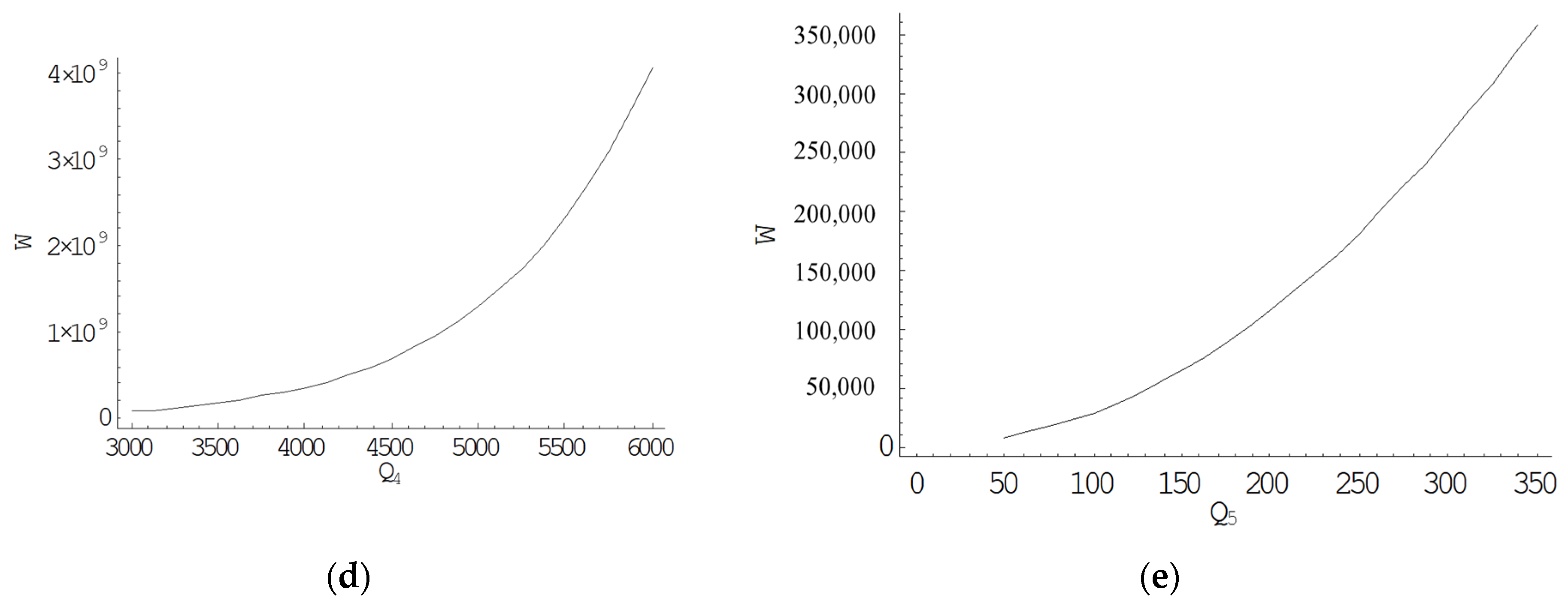
Figure 2a shows the convexity of the total cost function. In Figure 2b, after learning and forgetting, the second cycle is shown: as the quantity increases, initially, the total cost increases slightly, and after a certain value, it increases rapidly. In Figure 2c, it is analyzed that the total cost is less compared with cycle 2. In Figure 2d, it is analyzed that the total cost is less compared with cycle 3. In Figure 2e, it is analyzed that the total cost is less compared with cycle 4. Finally, as learning is used, there is more production improvement, and because of this, the total cost decreases.

5.2. Sensitivity Analysis

5.2.1. Effect of Slope of Learning Curve

The effect of the learning parameter is shown in Figure 3. Since r increases, production increases day by day. Therefore, the total cost decreases, and after a certain value of r, the total cost is slightly increased.

5.2.2. Effect of Carbon Emission Parameters

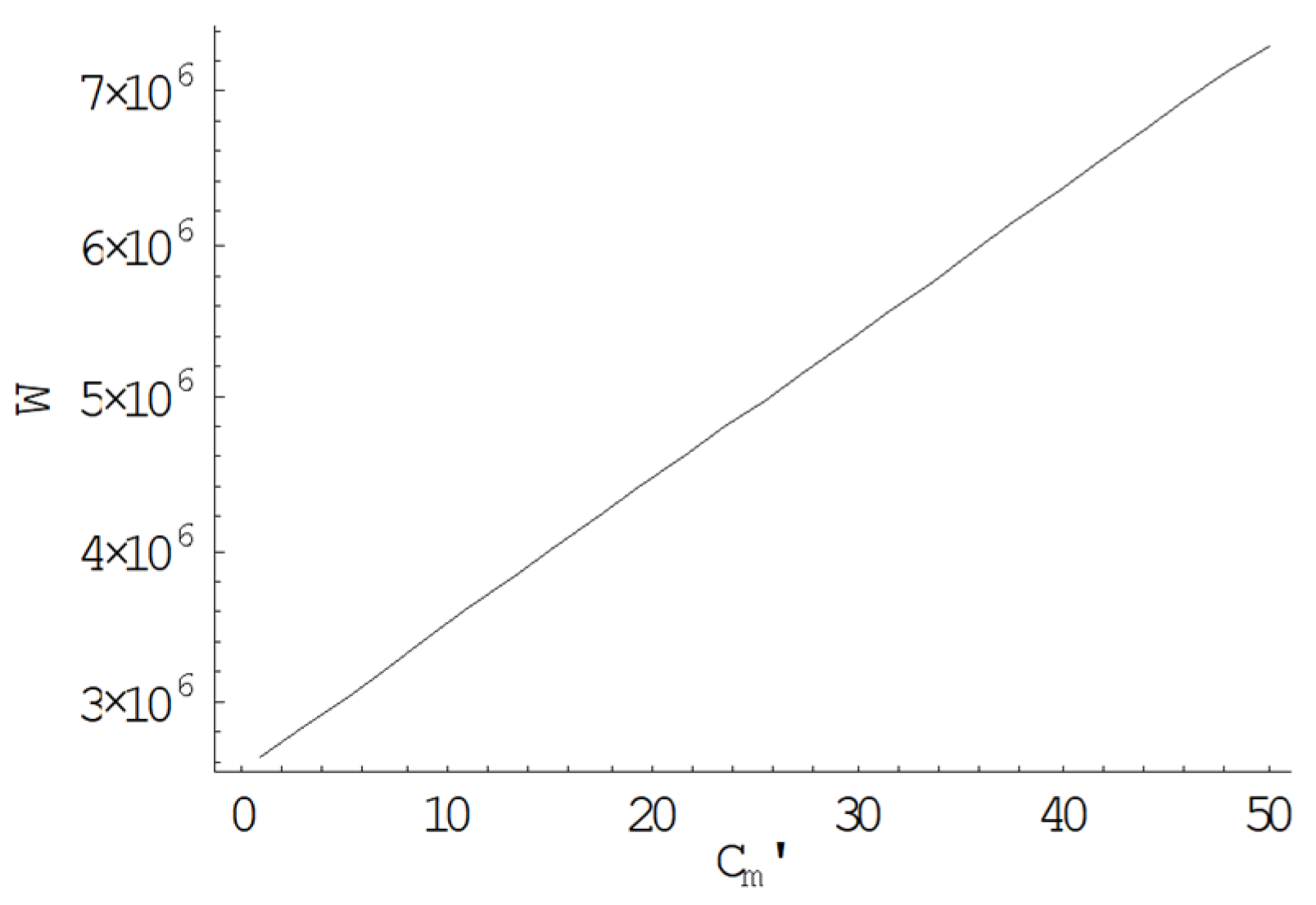
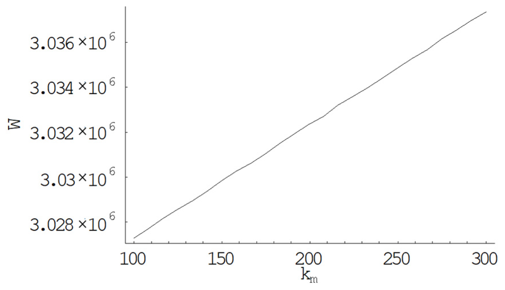
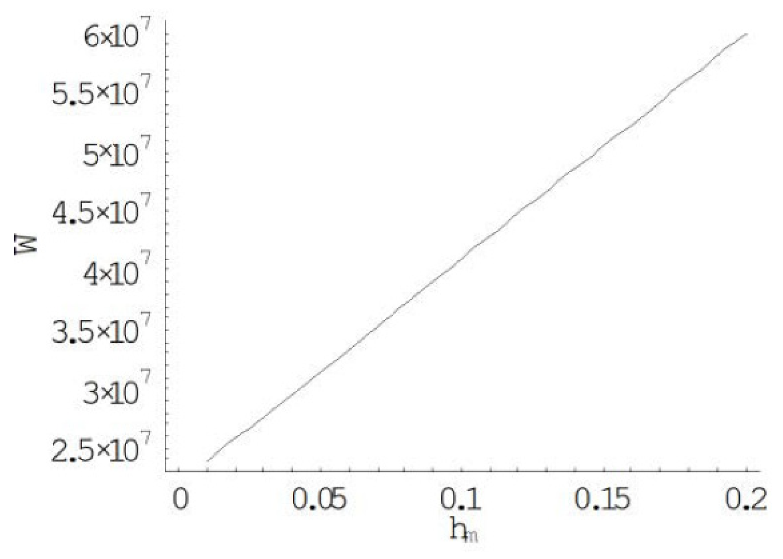
Carbon emissions could originate from many sources in the supply chain, such as the production process, setup process, deterioration process, warehousing, and transportation process. Only carbon emissions from the setup process, deterioration process, and warehousing are considered in this study. As the value of carbon emission cost parameters increases, the total cost increases, which is shown in Figure 4, Figure 5 and Figure 6.

5.2.3. Effect of Cost Parameters

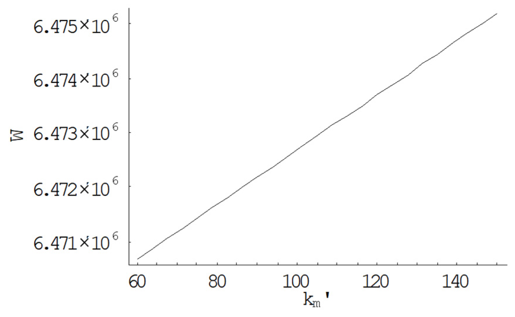
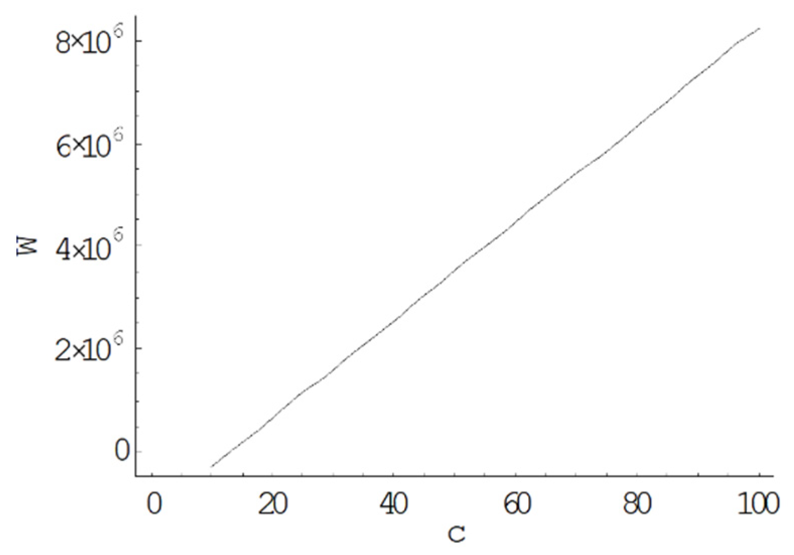
The effect of cost parameters on total cost is shown in Figure 7, Figure 8 and Figure 9. It is analyzed that as the value of the parameter increases, the total cost increases.

5.2.4. Effect of Parameters Used in Deterioration Rate

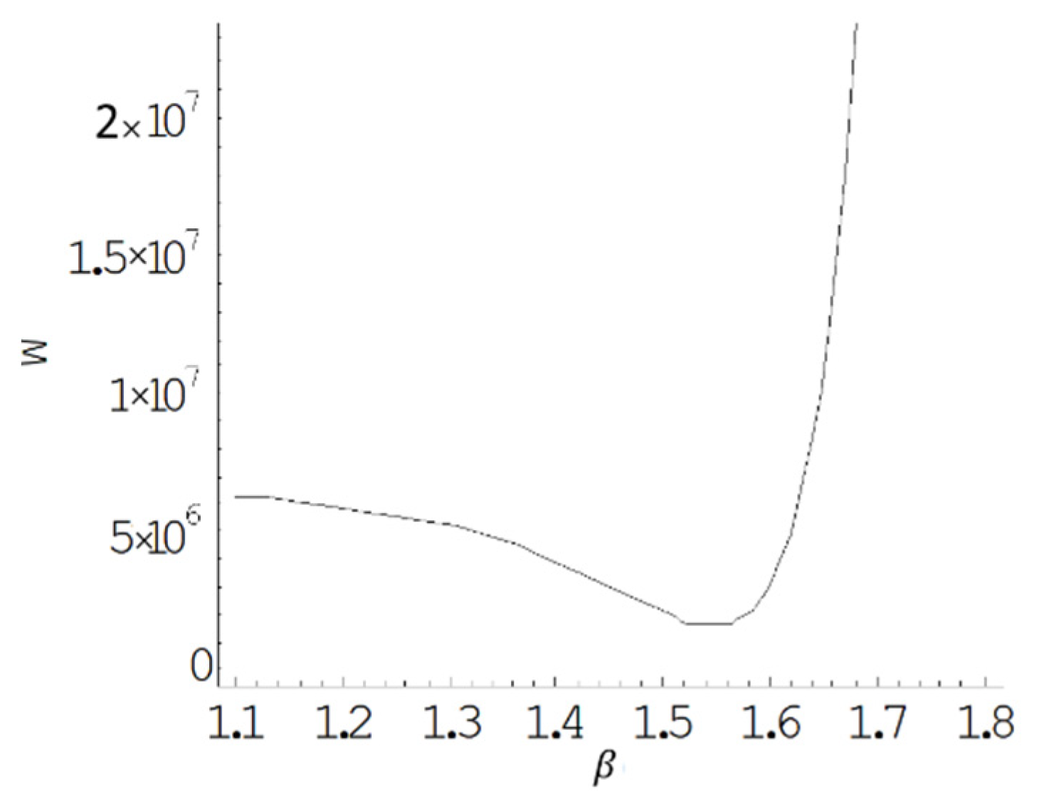
Some other parameters are used to represent the deterioration rate, which is sensitive to the model’s total cost (Figure 10 and Figure 11). Here, α is the scale parameter. As α increases, the total cost initially increases very slightly, but after a certain value, it increases very fast. β is the shape parameter; as β increases, the total cost decreases initially, and after a certain value, it increases very fast.

5.3. Effect of Parameters Used in Production Cost

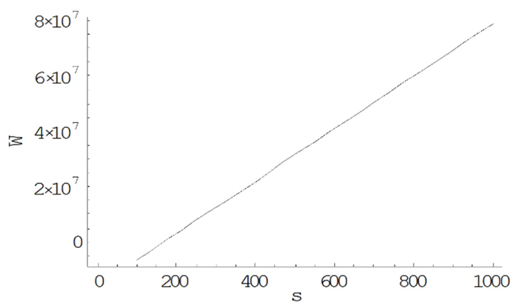
As the production cost parameters µ, s, and g increase, the total cost increases, which is shown in Figure 12, Figure 13 and Figure 14.

5.4. Managerial Insights

Based on the numerical results and sensitivity analysis, some recommendations can be suggested to the manager of industry.
The study considers LFL policy on which the production of industry depends. Figure 3 shows that the production rate increases and total cost decreases with an increase in the learning slope. However, after a certain limit, the total cost starts to increase. The manager of any industry should know how many days the learning policy should continue for each laborer.
The effect of carbon emissions on setup cost, holding cost, and deterioration cost are shown in Figure 4, Figure 5 and Figure 6. With increasing carbon emissions for setup or transportation, the total cost increases. The reduction in carbon emissions should be implemented to reduce the total cost of the supply chain along with the environmental benefits.
If the deterioration rate of products increases, the total supply chain cost increases. From (Figure 10 and Figure 11), it can be shown that initially, the total cost increases slightly, but after a certain deterioration rate, the total cost of the supply chain increases very fast. Thus, the industry should take care of the matter that the deterioration rate should be controllable.

6. Observations

The tabulated results are shown in Table 2, which indicates that the production time required for the first unit and the optimum quantity of production decrease with an increase in the number of production runs.
Produced optimum quantity and the cycle length are shown by columns three and seven, respectively, reflecting their decrease. This deduction is for the huge increase in the rate of production for successive cycles.
Learning and forgetting is a natural phenomenon that happens during production, but if we assume volume agility, we can minimize our loss and increase our production.
The major observation is about the learning rate. If the rate is increased, the total cost is decreased. However, after a certain amount of learning, the reduced total cost remains the same.
Because the agile production rate increases with the effect of the learning rate, the production rate increases with increasing value of the learning rate.
The introduction of carbon emissions in the cost parameters makes the model more effective.
In Figure 2, the effect of learning on total cost in each cycle is analyzed.

7. Conclusions

This paper examined the effect of learning–forgetting on the optimal lot size of production. Then, we extended the mathematical model for the LFL model as developed by Almari and Balkhi [20]. Due to the increasing value of the learning rate and a reduction in the forgetting rate, the production rate is increased, and the total cost were reduced. It is very important for a company to increase the learning rate to continually reduce the cost. The model obtained the minimum total cost when the forget slope was reduced the most among all others. The model’s generality was proved by the fact that the demand, production, and deterioration rates were arbitrary and known functions of time. The minimum break, in which the total forgetting was assumed to occur, had been considered as a function of the optimum quantity produced, then variable total forgetting breaks were allowed. Here, the rate of production was taken as the number of units remembered per unit of time, the demand rate was exponential for the manufacturer by allowing a deterioration rate that followed the Weibull distribution. The example showed the theoretical results under a partial transmission of learning, and its verification were given numerically with and without volume agility. The numerical outcomes reflected the effects of learning–forgetting incorporated in this model. If quality is considered, then the model can be extended again to improve quality [30]. If a retailer considers selling those products with a manufacturer to form supply chain management [31], that will be fruitful research, but supply chain players should be careful about unreliable players [45]. Any company may gain more by following the financial hypothesis [46]. Cross-docking policy can be applied [47] for the maximum flow of products. Carbon emissions can be reduced [48] by applying green technology to make a sustainable business.

Author Contributions

Conceptualization, B.S. and V.; Methodology, Supervision, S.R.S. and B.S.; Software, V.; Investigation, Formal analysis, Visualization, Project administration, Funding acquisition, Validation, B.S.; Data curation, Writing—original draft, V.; Writing—review & editing, V. and M.S. All authors have read and agreed to the published version of the manuscript.

Funding

This research received no external funding.

Data Availability Statement

Details are provided in the paper.

Conflicts of Interest

The authors declare no conflict of interest.

Appendix A

Notation

rSlope of the learning curve
Q(t)Number of units produced up to time t (units/cycle)
TComplete cycle time (days)
cmItem cost per unit per unit of time ($/unit)
cmCarbon emission cost due to deterioration per unit per unit of time ($/unit)
hmUnit holding cost per unit of time ($/unit/days)
hmCarbon emission cost from holding items in the warehouse per unit per unit of time ($/unit/days)
kmSetup cost per setup ($/setup)
kmCarbon emission cost due to transportation per order ($/order)
lSlope of forgetting
t11Time required to produce the first unit in the first cycle (days)
TijProduction time (days)
T2jInventory depletion time (days)
kMaterial cost ($/unit)
gDevelopment cost ($/unit)
sScaling parameter of tool/die cost ($/unit)
a,bScaling and shape paramter of demand, a > 0, b > 0, and a > b
α , β Scaling and shape paramter of deteriorateion rate

References

  1. Khouja, M. The economic production lot size model under volume flexibility. Comput. Oper. Res. 1995, 22, 515–523. [Google Scholar] [CrossRef]
  2. Khouja, M. The scheduling of economic lot size on volume flexibility production system. Int. J. Prod. Econ. 1997, 48, 73–86. [Google Scholar] [CrossRef]
  3. Sana, S.; Chaudhuri, K.S. On a volume flexible stock dependent inventory model. Adv. Model. Optim. 2003, 5, 197–210. [Google Scholar]
  4. Singh, S.R.; Singh, A.P.; Bhatia, D. A supply chain model with variable holding cost for flexible manufacturing system. Int. J. Oper. Res. Optim. 2010, 1, 107–120. [Google Scholar]
  5. Singh, S.R.; Gupta, V.; Gupta, P. EOQ model with volume agility, variable demand rate, Weibull deterioration rate and inflation. Int. J. Comput. Appl. 2013, 72, 1–6. [Google Scholar]
  6. Mehrotra, K.; Dem, H.; Singh, S.R.; Sharma, R. A volume flexible inventory model with trapezoidal demand under inflation. Pak. J. Stat. Oper. Res. 2014, 9, 429–442. [Google Scholar] [CrossRef] [Green Version]
  7. Singhal, S.; Singh, S.R. Modeling of an inventory model with multi variate demand under volume flexibility and learning. Uncertain Supply Chain. Manag. 2015, 3, 147–158. [Google Scholar] [CrossRef]
  8. Singh, S.R.; Gupta, V. Vendor-Buyer model with error in quality inspection and selling price dependent demand rate under the effect of volume agility. Int. J. Oper. Quant. Manag. 2016, 22, 357–371. [Google Scholar]
  9. Kamna, K.M.; Gautam, P.; Jaggi, C.K. Sustainable inventory policy for an imperfect production system with energy usage and volume agility. Int. J. Syst. Assur. Eng. Manag. 2020, 12, 44–52. [Google Scholar] [CrossRef]
  10. Sarkar, M.; Sarkar, B.; Dolgui, A. An Automated Smart Production with System Reliability Under a Leader-Follower Strategy of Supply Chain Management. In IFIP International Conference on Advances in Production Management Systems; Springer: Berlin/Heidelberg, Germany, 2022; pp. 459–467. [Google Scholar]
  11. Jauhari, W.A.; Pujawan, I.N.; Suef, M.; Govindan, K. Low carbon inventory model for vendor–buyer system with hybrid production and adjustable production rate under stochastic demand. Appl. Math. Model. 2022, 108, 840–868. [Google Scholar] [CrossRef]
  12. Jauhari, W.A.; Pujawan, N.; Suef, M. Sustainable inventory management with hybrid production system and investment to reduce defects. Ann. Oper. Res. 2022. [Google Scholar] [CrossRef]
  13. Wright, T. Factors affecting the cost of airplanes. J. Aeronaut. Sci. 1936, 3, 122–128. [Google Scholar] [CrossRef] [Green Version]
  14. Carlson, J.G.; Rowe, R.G. How much does forgetting cost? Ind. Eng. 1976, 8, 40–47. [Google Scholar]
  15. Elmaghraby, S.E. Economic manufacturing quantities under conditions of learning and forgetting (EMQ/LAF). Prod. Plan. Control 1990, 1, 196–208. [Google Scholar] [CrossRef]
  16. Jaber, M.Y.; Bonney, M. Production breaks and the learning curve: The forgetting phenomenon. Appl. Math. Model. 1996, 20, 162–169. [Google Scholar] [CrossRef]
  17. Jaber, M.Y.; Bonney, M. The economic manufacture/order quantity (EMQ/EOQ) and the learning curve: Past, present, and future. Int. J. Prod. Econ. 1999, 59, 93–102. [Google Scholar] [CrossRef]
  18. Jaber, M.Y.; Kher, H.V. The dual-phase learning–forgetting model. Int. J. Prod. Econ. 2002, 76, 229–242. [Google Scholar] [CrossRef]
  19. Balkhi, Z.T. The effect of learning on the optimal production lot size for deteriorating and partially backordered items with time varying demand and deterioration rates. Appl. Math. Model. 2003, 22, 763–779. [Google Scholar] [CrossRef] [Green Version]
  20. Alamri, A.A.; Balkhi, Z.T. The effects of learning and forgetting on the optimal production lot size for deteriorating items with time varying demand and deterioration rate. Int. J. Prod. Econ. 2007, 107, 125–138. [Google Scholar] [CrossRef]
  21. Jaber, M.Y.; Kher, H.V. Variant versus invariant time to total forgetting; the learn–forget curve model revisited. Comput. Ind. Eng. 2004, 46, 697–705. [Google Scholar] [CrossRef]
  22. Jaber, M.; Bonney, Y.; Moualek, I. Lot sizing with learning, forgetting and entropy. Int. J. Prod. Econ. 2009, 118, 19–25. [Google Scholar] [CrossRef]
  23. Das, D.; Roy, A.; Kar, S. A production inventory model for a deteriorating item incorporating learning effect using genetic algorithm. Adv. Oper. Res. 2011, 26, 146042. [Google Scholar] [CrossRef]
  24. Mahapatra, A.S.; Mahapatra, M.S.; Sarkar, B.; Majumder, S.K. Benefit of preservation technology with promotion and time-dependent deterioration under fuzzy learning. Expert Syst. Appl. 2022, 201, 117169. [Google Scholar] [CrossRef]
  25. Bachar, R.K.; Bhuniya, S.; Ghosh, S.K.; Sarkar, B. Controllable energy consumption in a sustainable smart manufacturing model considering superior service, flexible demand, and partial outsourcing. Mathematics 2022, 10, 4517. [Google Scholar] [CrossRef]
  26. Kumar, R.S.; Goswami, A. EPQ model with learning consideration, imperfect production and partial backlogging in fuzzy random environment. Int. J. Syst. Sci. 2015, 46, 1486–1497. [Google Scholar] [CrossRef]
  27. Kazemi, N.; Olugu, E.U.; Abdul-Rashid, S.H.; Ghazilla, R.A.R. A fuzzy EOQ model with backorders and forgetting effect on fuzzy parameters: An empirical study. Comput. Ind. Eng. 2016, 96, 140–148. [Google Scholar] [CrossRef]
  28. Ahmad, T.; Chen, H. Utility companies strategy for short-term energy demand forecasting using machine learning based models. Sustain. Cities Soc. 2018, 39, 401–417. [Google Scholar] [CrossRef]
  29. Batarfi, R.; Jaber, M.Y.; Glock, C.H. Pricing and inventory decisions in a dual-channel supply chain with learning and forgetting. Comput. Ind. Eng. 2019, 136, 397–420. [Google Scholar] [CrossRef]
  30. Marchi, B.; Zanoni, S.; Jaber, M.Y. Economic production quantity model with learning in production, quality, reliability and energy efficiency. Comput. Ind. Eng. 2019, 129, 502–511. [Google Scholar] [CrossRef]
  31. Marchi, B.; Zanoni, S.; Zavanella, L.E.; Jaber, M.Y. Green supply chain with learning in production and environmental investments. IFAC PapersOnLine 2018, 51, 1738–1743. [Google Scholar] [CrossRef]
  32. Sarkar, B.; Joo, J.; Kim, Y.; Park, H.; Sarkar, M. Controlling defective items in a complex multi-phase manufacturing system. RAIRO Oper. Res. 2022, 56, 871–889. [Google Scholar] [CrossRef]
  33. Sarkar, B.; Ganguly, B.; Pareek, S.; Cárdenas-Barrón, L.E. A three-echelon green supply chain management for biodegradable products with three transportation modes. Comput. Ind. Eng. 2022, 174, 108727. [Google Scholar] [CrossRef]
  34. Padiyar, S.V.S.; Vandana; Bhagat, N.; Singh, S.R.; Sarkar, B. Joint replenishment strategy for deteriorating multi-item through multi-echelon supply chain model with imperfect production under imprecise and inflationary environment. RAIRO Oper. Res. 2022, 56, 3071–3096. [Google Scholar] [CrossRef]
  35. Habib, M.S.; Omair, M.; Ramzan, M.B.; Chaudhary, T.N.; Farooq, M.; Sarkar, B. A robust possibilistic flexible programming approach toward a resilient and cost-efficient biodiesel supply chain network. J. Clean. Prod. 2022, 366, 132752. [Google Scholar] [CrossRef]
  36. Hota, S.K.; Ghosh, S.K.; Sarkar, B. Involvement of smart technologies in an advanced supply chain management to solve unreliability under distribution robust approach. AIMS Environ. Sci. 2022, 9, 461–492. [Google Scholar] [CrossRef]
  37. Yadav, D.; Singh, R.; Kumar, A.; Sarkar, B. Reduction of pollution through sustainable and flexible production by controlling by-products. J. Environ. Inform. 2022, 40, 106–124. [Google Scholar] [CrossRef]
  38. Moon, I.; Yun, W.Y.; Sarkar, B. Effects of variable setup cost, reliability, and production costs under controlled carbon emissions in a reliable production system. Eur. J. Ind. Eng. 2022, 16, 371–397. [Google Scholar] [CrossRef]
  39. Sarkar, B.; Kar, S.; Basu, K.; Guchhait, R. A sustainable managerial decision-making problem for a substitutable product in a dual-channel under carbon tax policy. Comput. Ind. Eng. 2022, 172, 108635. [Google Scholar] [CrossRef]
  40. Wangsa, I.D. Greenhouse gas penalty and incentive policies for a joint economic lot size model with industrial and transport emissions. Int. J. Ind. Eng. Comput. 2017, 8, 453–480. [Google Scholar]
  41. Marchi, B.; Zanoni, S.; Zavanella, L.E.; Jaber, M.Y. Supply chain models with greenhouse gases emissions, energy usage, imperfect process under different coordination decisions. Int. J. Prod. Econ. 2019, 211, 145–153. [Google Scholar] [CrossRef]
  42. Castellano, D.; Gallo, M.; Grassi, A.; Santillo, L.C. The effect of GHG emissions on production, inventory replenishment and routing decisions in a single vendor-multiple buyers supply chain. Int. J. Prod. Econ. 2019, 218, 30–42. [Google Scholar] [CrossRef]
  43. Daryanto, Y.; Wee, H.M.; Astanti, R.D. Three-echelon supply chain model considering carbon emission and item deterioration. Transp. Res. Part E: Logist. Transp. Rev. 2019, 122, 368–383. [Google Scholar] [CrossRef]
  44. Hariga, M.A.; Benkherouf, L. Optimal and heuristic inventory replenishment models for deteriorating items with exponential time-varying demand. Eur. J. Oper. Res. 1994, 79, 123–137. [Google Scholar] [CrossRef]
  45. Hota, S.K.; Ghosh, S.K.; Sarkar, B. A solution to the transportation hazard problem in a supply chain with an unreliable manufacturer. AIMS Environ. Sci. 2022, 9, 354–380. [Google Scholar] [CrossRef]
  46. Oryani, B.; Moridian, A.; Sarkar, B.; Rezania, S.; Kamyab, H.; Khan, M.K. Assessing the financial rеsоurсе curse hypothesis in Iran: Thе nоvеl dynаmiс АRDL approach. Resour. Policy 2022, 78, 102899. [Google Scholar] [CrossRef]
  47. Mukherjee, T.; Sangal, I.; Sarkar, B.; Alkadash, T.M. Mathematical estimation for maximum flow of goods within a cross-dock to reduce inventory. Math. Biosci. Eng. 2022, 19, 13710–13731. [Google Scholar] [CrossRef]
  48. Mishra, M.; Ghosh, S.K.; Sarkar, B. Maintaining energy efficiencies and reducing carbon emissions under a sustainable supply chain management. AIMS Environ. Sci. 2022, 9, 603–635. [Google Scholar] [CrossRef]
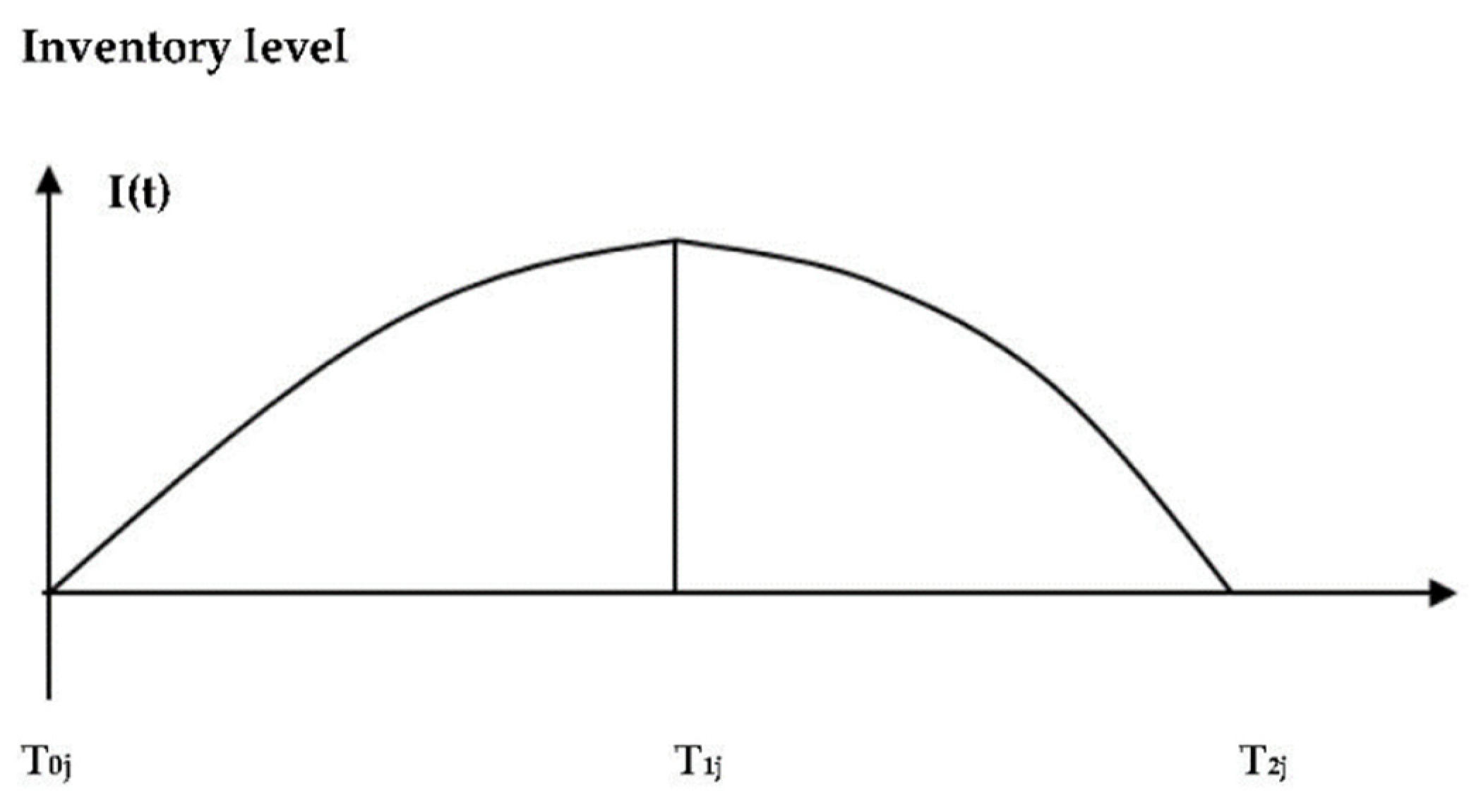
Figure 1. Inventory level of manufacturer under learning and forgetting.
Mathematics 11 00368 g001
Figure 2. Graphical representation of convexity: (a) convexity of the total cost function versus the number of units for cycle 1; (b) convexity of the total cost function versus the number of units for cycle 2; (c) convexity of the total cost function versus the number of units for cycle 3; (d) convexity of the total cost function versus the number of units for cycle 4; (e) convexity of the total cost function versus the number of units for cycle 5.
Mathematics 11 00368 g002aMathematics 11 00368 g002b
Figure 3. Graphical representation of convexity of the total cost function versus the number of units.
Mathematics 11 00368 g003
Figure 4. Total cost versus carbon emission parameter cm.
Mathematics 11 00368 g004
Figure 5. Total cost versus carbon emission parameter hm.
Mathematics 11 00368 g005
Figure 6. Total cost versus carbon emission parameter km’.
Mathematics 11 00368 g006
Figure 7. Total cost versus parameter c.
Mathematics 11 00368 g007
Figure 8. Total cost versus parameter km.
Mathematics 11 00368 g008
Figure 9. Total cost versus parameter hm.
Mathematics 11 00368 g009
Figure 10. Total cost versus parameter α.
Mathematics 11 00368 g010
Figure 11. Total cost versus parameter β.
Mathematics 11 00368 g011
Figure 12. Total cost versus parameter µ.
Mathematics 11 00368 g012
Figure 13. Total cost versus parameter s.
Mathematics 11 00368 g013
Figure 14. Total cost versus parameter g.
Mathematics 11 00368 g014
Table 1. Contribution from various researchers.
ResearchersModelManufacturing TypePolicyDemand PatternEnvironment
Khouja [1,2]EPQVolume flexibilityNot applicableConstantNot applicable
Singh et al. [5]EPQVolume agilityNot applicableVariableInflation
Singhal and Singh [7]EPQVolume agilityNot applicableVariableNot applicable
Kamna et al. [9]EPQVolume agilitySustainableVariableEnergy usage
Elmaghraby [15]EPQTraditionalLFCMVariableNot applicable
Jaber and Boney [16]EOQNot applicableLFCMConstantNot applicable
Jaber and Kher [18]EOQNot applicableDual
Phase LFCM
ConstantNot applicable
Balkhi [19]EPQTraditionalLearningVariableNot applicable
Alamri and Balkhi [20]EPQTraditionalLFCMVariableNot applicable
Das et al. [23]EPQTraditionalLearning, genetic algorithmConstantNot applicable
Mahapatra et al. [24]EPQNot applicableLearningUncertainFuzzy
Bachar et al. [25]EPQSmartNot applicableVariableNot applicable
Kumar and Goswami [26]EPQTraditionalLearningUncertainFuzzy
Batarfi et al. [29]SCMTraditionalLFCMVariableNot applicable
Sarkar et al. [33]SCMTraditionalNot applicableVariableCarbon emission
This paperEPQVolume agilityLFCMVariableCarbon emission and Weibull deterioration rate
EPQ, economic production model; LFCM, learn–forget curve model; SCM, supply chain management.
Table 2. Optimal solutions with the partial transmission of learning for Example 1.
Cycle no. jRequired Time to Produce First Unit
t1j (Days)
Produced Units in
[T0j, T1j]
Qj (Units/Cycle)
No. of Units Remembered in
[T0j, T2j]
ηj+1
Production Period
T1j (Days)
Production Rate by Time T1j is
P(T1j) (Units)
Consumption
Period
T2j (Days)
Qj + RjIntercept of the
Forgetting Curve
t 1 j ^
Forgetting Slo pe
lj
Minimum
Total Cost
W ($/Cycle)
10.06518881896.8261.6634.0280.2925290.02960.00253.0325 × 106
20.02983828143.1210985.140235,5780.01150.00242.89 × 1012
30.01176557.246366.33525.8133.628,6830.00480.00231.631 × 1010
40.00493181.1930677.73457.139.7319,5900.00220.00221.136 × 108
50.0021155.778148.940.23753.0411.7331,470.120.00130.002169,532.70
Disclaimer/Publisher’s Note: The statements, opinions and data contained in all publications are solely those of the individual author(s) and contributor(s) and not of MDPI and/or the editor(s). MDPI and/or the editor(s) disclaim responsibility for any injury to people or property resulting from any ideas, methods, instructions or products referred to in the content.