Solving Optimization Problems Using an Extended Gradient-Based Optimizer

Abstract

This paper proposes an improved method for solving diverse optimization problems called EGBO. The EGBO stands for the extended gradient-based optimizer, which improves the local search of the standard version of the gradient-based optimizer (GBO) using expanded and narrowed exploration behaviors. This improvement aims to increase the ability of the GBO to explore a wide area in the search domain for the giving problems. In this regard, the local escaping operator of the GBO is modified to apply the expanded and narrowed exploration behaviors. The effectiveness of the EGBO is evaluated using global optimization functions, namely CEC2019 and twelve benchmark feature selection datasets. The results are analyzed and compared to a set of well-known optimization methods using six performance measures, such as the fitness function’s average, minimum, maximum, and standard deviations, and the computation time. The EGBO shows promising results in terms of performance measures, solving global optimization problems, recording highlight accuracies when selecting significant features, and outperforming the compared methods and the standard version of the GBO.

1. Introduction

Nowadays, data volumes are increasing daily, massively, and rapidly; data include many features and attributes, and some of these attributes may be irrelevant or redundant. However, such data should be saved, processed, and retrieved with reasonable computational time and effort. Therefore, using data processing techniques in terms of volume and compatibility is essential; one of these techniques is the feature selection strategy, which is used to select the essential sub-features. In this context, searching for the best attributes in many features is considered a challenge. Therefore, many feature selection models have been proposed to help solve that problem. For instance, the authors of [1] proposed a modified version of the salp swarm algorithm (SSA) called DSSA to reduce the features of different benchmark datasets; the results showed the effectiveness of the DSSA and good classification accuracy compared to the other methods. Another work was performed by the authors of [2]; they introduced a feature selection stage to detect facial expressions from a real dataset using the sine–cosine algorithm (SCA); their method reduced the feature number by 87%.

Furthermore, the authors of [3] applied the particle swarm optimization (PSO) and fuzzy rough set to reduce the feature set of benchmark datasets. The obtained feature sets were evaluated using the decision tree and naive Bayes classifiers; the results showed their effectiveness at evaluating the selected features. The e-Jaya optimization algorithm was also effectively utilized by the authors of [4] to select the essential features in the group of essays to grade them in less time with more accuracy. In this context, the feature selection was applied in medical applications, such as [5]; it was applied to help classify the influenza A virus cases; the results showed good performances compared to the classic methods. The whale optimization algorithm (WOA) was also applied in feature selection by the authors of [6]. In that study, the WOA was enhanced by a pooling mechanism. The performance of the enhanced WOA was evaluated using two experiments: global optimization and feature selection. It was also evaluated in detecting the coronavirus disease (COVID-19). The results showed the efficiency of the enhanced WOA in solving different problems. More applications for feature selection can be found here [7,8,9,10,11].

From this insight, this paper proposes a new method for feature selection. The proposed method, called EGBO, improves the gradient-based optimizer (GBO) using expanded and narrowed exploration behaviors of the Aquila optimizer (AO) [12]. The effectiveness of the EGBO was evaluated using seven well-known benchmark feature selection datasets and compared with some optimization algorithms.

The gradient-based optimizer is a recent optimization algorithm that was motivated by the gradient-based Newton method [13]. It has been successfully applied to several applications, such as identifying the parameters of photovoltaic systems [14]. The GBO was also applied by [15] to predict the infected, recovered, and death cases for the COVID-19 pandemic in the US. On the other hand, the aquila optimizer (AO) is a recent optimization algorithm; it simulates the hunting behaviors of the Aquila proposed by [12]. The AO was used in several applications, such as forecasting oil production [16] and forecasting China’s rural community population [17]. Furthermore, the authors of [18] applied the GBO to identify the parameters in photovoltaic models. Their method’s performance was evaluated using the single-diode, double-diode, and three-diode models as well as the photovoltaic module model. The results showed that their method obtained the best results and it was highly competitive with the compared technologies. On the same side, the authors of [19] used an improved version of the GBO, called IGBO, for parameter extraction of photovoltaic models. The IGBO used two strategies to identify the adaptive parameters: adaptive weights and chaotic behavior. The results showed competitive performance compared to the other methods. Furthermore, the GBO was also modified and called GBOSMA by the authors of [20]. They applied the slime mould algorithm (SMA) as a local search to improve the GBOSMA to explore the search space; the experimental results demonstrated the superiority of their method. In this regard, the difference between the GBOSMA and this paper can be summarized as follows; the GBOSMA uses a probability to apply the operator of the SMA, whereas this paper extends the local search operator of the GBO using the expanded and narrowed exploration behaviors of the AO algorithm.

From the above studies, the GBO was used in different applications and showed promising results; it also has some advantages, such as ease of use and not having many predefined parameters that need to be optimized. However, it may show slow convergence in some cases and can be trapped in local optima; therefore, this paper introduces a new version of the GBO called EGBO to improve the local search phase of the standard GBO method.

The rest of this paper is arranged as follows: Section 2 describes the methods and materials used in this paper. Section 3 describes the proposed method. The experiments and results are presented in Section 4. Section 5 concludes the paper and lists future works.

2. Gradient-Based Optimizer

This section introduces a brief description of the gradient-based optimizer (GBO). The GBO is an optimization algorithm proposed by [13]. The optimization process of the GBO contains two main phases: gradient search rule (GSR) and local escaping operator (LEO). These phases are explained in the following subsections.

2.1. Gradient Search Rule (GSR)

The GSR is used to promote the GBO exploration. The following equations are applied to perform the GSR and to update the position $\left(x_n^l\right)$.

$$X{1}_n^l=x_n^l-randn\times {\rho }_1\times \frac{2\Delta x\times x_n^l}{(X_{worst}-X_{best}+\epsilon )}+rand\times {\rho }_2\times (X_{best}-x_n^l)$$

(1)

$${\rho }_1=2\times rand\times \alpha -\alpha$$

(2)

$$\alpha =|\beta \times sin(\frac{3\pi }{2}+sin(\beta \times \frac{3\pi }{2}))|$$

(3)

$$\beta ={\beta }_{min}+({\beta }_{max}-{\beta }_{min})\times {(1-{(\frac{l}{L})}^3)}^2$$

(4)

where ${\beta }_{min}=0.20$ and ${\beta }_{max}=1.20$. l and L denote the current and total iterations. $\epsilon$ is a random value $\in [0,0.1]$. $randn$ denotes a normally distributed number. ${\rho }_2$ is computed using Equation (5).

$${\rho }_2=2\times rand\times \alpha -\alpha$$

(5)

$$\Delta x=rand(1:N)\times \mid step\mid$$

(6)

$$step=\frac{(X_{best}-x_{r1}^l)+\delta }{2}$$

(7)

$$\delta =2\times rand\times (|\frac{x_{r1}^l+x_{r2}^l+x_{r3}^l+x_{r4}^l}{4}-x_n^l|)$$

(8)

where $r_1$, $r_2$, $r_3$, $r_4$ and $rand$ denote random numbers $\in [1,N]$. In this stage, the $X{2}_n^l$ is computed as in Equation (9).

$$X{2}_n^l=X_{best}-randn\times {\rho }_1\times \frac{2\Delta x\times x_n^l}{(y{p}_n^l-y{q}_n^l+\epsilon )}+rand\times {\rho }_2\times (x_{r1}^l-x_{r2}^l)$$

(9)

$$y{p}_n=rand\times (\frac{[z_{n+1}+x_n]}{2}+rand\times \Delta x)$$

(10)

$$y{q}_n=rand\times (\frac{[z_{n+1}+x_n]}{2}-rand\times \Delta x)$$

(11)

After that, the solution of the next loop $X_n^{m+1}$ is computed, as in Equation (12) based on $X{1}_n^l$ and $X{2}_n^l$ and the current solution $X_n^l$.

$$X_n^{m+1}=r_a\times (r_b\times X{1}_n^l+(1-r_b)\times X{2}_n^l)+(1-r_a)\times X{3}_n^l$$

(12)

$$X{3}_n^l=X_n^l-{\rho }_1\times (X{2}_n^l-X{1}_n^l)$$

(13)

2.2. Local Escaping Operator (LEO)

The LEO is applied to improve the efficiency of the GBO algorithm. This phase starts if a random number ($pr$) exceeds $0.5$. It also uses another random number ($pr2$) to update the solutions using Equation (14) if $pr2>0.5$; otherwise, it will update the solution using Equation (15).

$$\begin{array}{cc}\hfill X_n^{l+1}=& X_n^{l+1}+f_1\times (u_1\times X_{best}-u_2\times x_k^l)+\hfill \\ \hfill & f_2\times {\rho }_1\times (u_3\times (X{2}_n^l-X{1}_n^l)+u_2\times (x_{r1}^l-x_{r2}^l))/2\hfill \end{array}$$

(14)

$$\begin{array}{cc}\hfill X_n^{l+1}=& X_{best}+f_1\times (u_1\times X_{best}-u_2\times x_k^l)+\hfill \\ \hfill & f_2\times {\rho }_1\times (u_3\times (X{2}_n^l-X{1}_n^l)+u_2\times (x_{r1}^l-x_{r2}^l))/2\hfill \end{array}$$

(15)

where $x_{r1}^m$, $x_{r2}^m$, and $x_k^m$ are random solutions. $f_1$ and $f_2$ are random numbers. $u_1$, $u_2$, and $u_3$ are generated as in Equations (16)–(18).

$$u_1=\{\begin{array}{c}2\times randif{\lambda }_1<0.5\hfill \\ 1otherwise\hfill \end{array}$$

(16)

$$u_2=\{\begin{array}{c}randif{\lambda }_1<0.5\hfill \\ 1otherwise\hfill \end{array}$$

(17)

$$u_3=\{\begin{array}{c}randif{\lambda }_1<0.5\hfill \\ 1otherwise\hfill \end{array}$$

(18)

where $rand$ and ${\lambda }_1$ are generated randomly $\in [0,1]$. $x_k^l$ in computed as in Equation (19).

$$x_k^l=L_2\times x_p^l+(1-L_2)\times x_{rand}$$

(19)

where $L_2$ is a binary variable generated randomly. Algorithm 1 shows the structure of the GBO.

Algorithm 1 Gradient-based optimizer.

1: Define the global parameters $L,N$, and D, as well as the initial population, X. 2: Compute the fitness function for population X. 3: Select the best solution $X_{best}^m$ and the worst one $X_{worst}^m$. 4: Start the main optimization process. 5: forl=1 to Ldo 6:     for n = 1: N do 7:         for i = 1: D do 8:            Generate the random variables to apply GSR. 9:            Update the current position using the GSR phase. 10:         end for 11:         Generate the random variables to apply LEO. 12:         if $rand\left(\right)<0.5$ then 13:            Update the current position using the LEO phase. 14:         end if 15:         Update the best and worst positions. 16:     end for 17: end for 18: Return the best result.

3. Proposed Method

This section explains the structure of the proposed EGBO method. The EGBO aims to improve the exploration phase of the standard GBO by using Lévy flight as well as the expanded and narrowed exploration behaviors of the AO algorithm [12]. In this regard, the local escaping operator of the GBO is extended to include the expanded and narrowed exploration behaviors. This modification adds more flexibility and reliability to the GBO to explore different hidden areas in the search space, reflecting on effectively reaching the optimal point.

The EGBO starts by generating its population as in Equation (20), then evaluates it to determine the best solutions.

$$X=r(N,D)\times (lb-ub)+lb$$

(20)

where N and D denote the population size and dimension, respectively, of the given problem. r is a random function. $lb$ and $ub$ denote the lower and upper bounds.

Then, the GSR is applied to accelerate the convergence behavior. After that, the local escaping operator phase is used to maintain the current solution. In this stage, a random variable ($rand$) is checked to run the improvement phase. This phase runs an expanded or narrowed exploration (using a random variable). Therefore, if $rand2\left(\right)>0.5$, run the expanded exploration; else, run the narrowed exploration.

The EGBO uses Equation (21) to apply the expanded exploration as follows:

$$X=X_{best}\times (\frac{1-l}{L})+(X_a-X_{best})\times rand\left(\right)$$

(21)

where $X_{best}$ denotes the best solution so far. l and L denote the current and total iterations. $X_a$ is the average of the current solution, and it is calculated as:

$$X_a=\frac{1}{N}(\sum _{i=1}^N{x}_i)$$

(22)

Furthermore, the EGBO uses Equation (23) to apply the narrowed exploration. It also applies the Lévy flight distribution to update the solutions as follows:

$$X=X_{best}\times Lvy\left(D\right)+X_r+(y-q)\times rand\left(\right)$$

(23)

where $Lvy\left(D\right)$ applies the Lévy flight distribution as in Equations (24) and (25). $X_r$ is a random solution.

$$Lvy\left(D\right)=s\times \frac{u\times \sigma }{{\left|\delta \right|}^{\frac{1}{{\beta }_3}}}$$

(24)

$$\sigma =(\frac{\Gamma (1+{\beta }_3)\times sine\left(\frac{\pi {\beta }_3}{2}\right)}{\Gamma \left(\frac{1+{\beta }_3}{2}\right)\times {\beta }_3\times 2^{\left(\frac{{\beta }_3-1}{2}\right)}})$$

(25)

where $s=0.010$ and ${\beta }_3=1.50$. u and $\delta$ denote random numbers ∈ [0,1]. y and q are two variables that simulate the spiral shape, and they are calculated as in Equations (26)–(28), respectively.

$$y=r\times cos\left(\theta \right),q=r\times sin\left(\theta \right)$$

(26)

$$r=r_0+U\times d_1,d_1=1,2,\cdots ,D$$

(27)

$$\theta =-\omega \times d_1+{\theta }_1,{\theta }_1=\frac{3\times \pi }{2}$$

(28)

where $r_0$ is a random value $\in [0,10]$. $U=0.005650$ and $\omega =0.0050$, these values are selected based on the recommendation of the AO study [12].

After that, the best solution is determined and saved using the fitness function. This sequence is repeated until the stop condition is reached. Finally, the best result is presented. Algorithm 2 shows the pseudo-code of the proposed EGBO method.

Algorithm 2 Pseudo-code of the proposed EGBO method.

1: First: Define the global parameters $L,N$, and D, as well as the initial population X. 2: Perform the fitness function to evaluate the population to define the best solution $X_{best}$ and the worst one $X_{worst}$. 3: Second: Start the main processing. 4: for  $l=1:L$do 5:     for $n=1:N$ do 6:         for $i=1:D$ do 7:            Generate random variables. 8:            Update the current position using the GSR phase. 9:         end for 10:       Start the LEO phase 11:       if $rand<0.5$ then 12:            Compute the solution using the LEO phase. 13:            if $rand<0.5$ then 14:                if $rand<0.5$ then 15:                    Apply the expanded exploration. 16:                else 17:                    Apply the narrowed exploration. 18:                end if 19:            end if 20:         end if 21:         Update the best and worst positions. 22:     end for 23: end for 24: Return the best result.

4. Experiment and Results

In this section, the proposed EGBO is evaluated in two experiments; the first is global optimization, and the second is feature selection. All results of the proposed EGBO are compared to six algorithms: GBO, particle swarm optimization (PSO) [21], genetic algorithms (GA) [22], differential evolution (DE) [23], dragonfly algorithm (DA) [24], and moth-flame optimization (MFO) [25]. These algorithms are selected because they have shown stability and good results in the literature. They have different behaviors in exploring the search space; for instance, the PSO uses the particle’s position and velocity, whereas the GA uses three phases: selection, crossover, and mutation.

The parameters of all algorithms were set as mentioned in their original paper, whereas the global parameters were as follows: the search agents’ numbers = 25 and the maximum iteration number = 100. The number of the fitness function evaluation is set to 2500 as a stop condition, and each algorithm is applied with 30 independent runs.

4.1. First Experiment: Solving Global Optimization Problem

In this section, the proposed EGBO method is assessed using CEC2019 [26] benchmark functions to solve global optimization functions and the results are compared to some well-known algorithms. This experiment aims to evaluate the proposed EGBO in solving different types of test functions.

The comparison is performed using a set of performance measures: the mean (Equation (29)), min, max, and standard deviations (Equation (30)) of the fitness functions, and the computation times for all algorithms. All experimental results are listed in

Table 1. Results of the average measure of the fitness function values.

	EGBO	GBO	PSO	GA	MFO	DA	DE	AO
F1	4.43 $\times {\mathbf{10}}^{\mathbf{4}}$	5.01 $\times {10}^4$	5.83 $\times {10}^{12}$	6.19 $\times {10}^{10}$	5.60 $\times {10}^{10}$	7.14 $\times {10}^{10}$	1.49 $\times {10}^{11}$	7.53 $\times {10}^4$
F2	1.73 $\times {\mathbf{10}}^{\mathbf{1}}$	1.73 $\times {10}^1$	1.70 $\times {10}^4$	2.61 $\times {10}^1$	1.74 $\times {10}^1$	4.10 $\times {10}^1$	1.82 $\times {10}^1$	1.75 $\times {10}^1$
F3	1.27 $\times {\mathbf{10}}^{\mathbf{1}}$	1.27 $\times {10}^1$	1.27 $\times {10}^1$	1.27 $\times {10}^1$	1.27 $\times {10}^1$	1.27 $\times {10}^1$	1.27 $\times {10}^1$	1.27 $\times {10}^1$
F4	7.62 $\times {\mathbf{10}}^{\mathbf{1}}$	9.22 $\times {10}^1$	3.68 $\times {10}^3$	1.27 $\times {10}^2$	2.13 $\times {10}^2$	9.09 $\times {10}^2$	8.84 $\times {10}^1$	3.61 $\times {10}^3$
F5	1.18 $\times {\mathbf{10}}^{\mathbf{0}}$	1.19 $\times {10}^0$	2.58 $\times {10}^0$	1.19 $\times {10}^0$	1.38 $\times {10}^0$	1.59 $\times {10}^0$	1.61 $\times {10}^0$	2.29 $\times {10}^0$
F6	1.17 $\times {10}^1$	1.20 $\times {10}^1$	1.09 $\times {10}^1$	7.65 $\times {10}^0$	7.21 $\times {\mathbf{10}}^{\mathbf{0}}$	8.80 $\times {10}^0$	1.06 $\times {10}^1$	1.19 $\times {10}^1$
F7	4.30 $\times {10}^2$	4.68 $\times {10}^2$	4.31 $\times {10}^2$	3.38 $\times {\mathbf{10}}^{\mathbf{2}}$	3.58 $\times {10}^2$	6.55 $\times {10}^2$	6.34 $\times {10}^2$	7.20 $\times {10}^2$
F8	6.00 $\times {10}^0$	5.86 $\times {10}^0$	5.78 $\times {10}^0$	5.41 $\times {\mathbf{10}}^{\mathbf{0}}$	5.76 $\times {10}^0$	5.92 $\times {10}^0$	6.51 $\times {10}^0$	6.34 $\times {10}^0$
F9	3.01 $\times {\mathbf{10}}^{\mathbf{0}}$	3.41 $\times {10}^0$	1.59 $\times {10}^2$	3.44 $\times {10}^0$	4.08 $\times {10}^0$	3.10 $\times {10}^1$	3.23 $\times {10}^0$	2.68 $\times {10}^2$
F10	2.06 $\times {10}^1$	2.06 $\times {10}^1$	2.05 $\times {10}^1$	2.02 $\times {10}^1$	2.01 $\times {\mathbf{10}}^{\mathbf{1}}$	2.02 $\times {10}^1$	2.04 $\times {10}^1$	2.06 $\times {10}^1$

Boldface indicates the best result.

,

Table 2. Results of the Std measure of the fitness function values.

	EGBO	GBO	PSO	GA	MFO	DA	DE	AO
F1	3.23 $\times {\mathbf{10}}^{\mathbf{3}}$	6.44 $\times {10}^3$	3.17 $\times {10}^{12}$	8.14 $\times {10}^{10}$	4.80 $\times {10}^{10}$	9.09 $\times {10}^{10}$	6.23 $\times {10}^{10}$	1.74 $\times {10}^4$
F2	2.79 $\times {\mathbf{10}}^{-\mathbf{5}}$	6.89 $\times {10}^{-5}$	4.73 $\times {10}^3$	2.51 $\times {10}^1$	1.77 $\times {10}^{-2}$	7.29 $\times {10}^1$	5.83 $\times {10}^{-1}$	8.72 $\times {10}^{-2}$
F3	6.76 $\times {\mathbf{10}}^{-\mathbf{11}}$	3.36 $\times {10}^{-9}$	4.44 $\times {10}^{-4}$	1.06 $\times {10}^{-6}$	2.61 $\times {10}^{-4}$	7.28 $\times {10}^{-4}$	4.27 $\times {10}^{-5}$	3.75 $\times {10}^{-5}$
F4	3.73 $\times {10}^1$	6.89 $\times {10}^1$	2.54 $\times {10}^3$	8.82 $\times {10}^1$	3.16 $\times {10}^2$	7.30 $\times {10}^2$	1.34 $\times {\mathbf{10}}^{\mathbf{1}}$	1.43 $\times {10}^3$
F5	7.45 $\times {\mathbf{10}}^{-\mathbf{2}}$	1.14 $\times {10}^{-1}$	7.45 $\times {10}^{-1}$	1.21 $\times {10}^{-1}$	1.62 $\times {10}^{-1}$	2.41 $\times {10}^{-1}$	9.31 $\times {10}^{-2}$	2.19 $\times {10}^{-1}$
F6	8.67 $\times {10}^{-1}$	5.07 $\times {\mathbf{10}}^{-\mathbf{1}}$	9.32 $\times {10}^{-1}$	1.05 $\times {10}^0$	1.60 $\times {10}^0$	1.70 $\times {10}^0$	5.43 $\times {10}^{-1}$	8.56 $\times {10}^{-1}$
F7	1.96 $\times {10}^2$	2.38 $\times {10}^2$	2.32 $\times {10}^2$	1.87 $\times {10}^2$	2.06 $\times {10}^2$	3.03 $\times {10}^2$	1.26 $\times {10}^2$	2.64 $\times {10}^2$
F8	3.57 $\times {\mathbf{10}}^{-\mathbf{1}}$	6.77 $\times {10}^{-1}$	8.36 $\times {10}^{-1}$	7.76 $\times {10}^{-1}$	6.22 $\times {10}^{-1}$	6.22 $\times {10}^{-1}$	3.74 $\times {10}^{-1}$	5.90 $\times {10}^{-1}$
F9	2.62 $\times {\mathbf{10}}^{-\mathbf{1}}$	5.56 $\times {10}^{-1}$	2.40 $\times {10}^2$	6.62 $\times {10}^{-1}$	8.12 $\times {10}^{-1}$	5.91 $\times {10}^1$	3.13 $\times {10}^{-1}$	1.29 $\times {10}^2$
F10	6.56 $\times {\mathbf{10}}^{-\mathbf{2}}$	1.44 $\times {10}^{-1}$	1.54 $\times {10}^{-1}$	7.52 $\times {10}^{-2}$	1.20 $\times {10}^{-1}$	1.33 $\times {10}^{-1}$	6.65 $\times {10}^{-2}$	1.08 $\times {10}^{-1}$

Boldface indicates the best result.

,

Table 3. Results of the max measure of the fitness function values.

	EGBO	GBO	PSO	GA	MFO	DA	DE	AO
F1	5.23 $\times {\mathbf{10}}^{\mathbf{4}}$	6.21 $\times {10}^4$	1.70 $\times {10}^{13}$	3.26 $\times {10}^{11}$	1.97 $\times {10}^{11}$	4.12 $\times {10}^{11}$	3.05 $\times {10}^{11}$	1.23 $\times {10}^5$
F2	1.73 $\times {\mathbf{10}}^{\mathbf{1}}$	1.73 $\times {10}^1$	2.55 $\times {10}^4$	1.52 $\times {10}^2$	1.74 $\times {10}^1$	3.80 $\times {10}^2$	1.94 $\times {10}^1$	1.76 $\times {10}^1$
F3	1.27 $\times {\mathbf{10}}^{\mathbf{1}}$	1.27 $\times {10}^1$	1.27 $\times {10}^1$	1.27 $\times {10}^1$	1.27 $\times {10}^1$	1.27 $\times {10}^1$	1.27 $\times {10}^1$	1.27 $\times {10}^1$
F4	1.81 $\times {10}^2$	3.27 $\times {10}^2$	1.03 $\times {10}^4$	3.49 $\times {10}^2$	1.76 $\times {10}^3$	2.96 $\times {10}^3$	1.15 $\times {\mathbf{10}}^{\mathbf{2}}$	5.80 $\times {10}^3$
F5	1.29 $\times {\mathbf{10}}^{\mathbf{0}}$	1.53 $\times {10}^0$	4.68 $\times {10}^0$	1.52 $\times {10}^0$	1.81 $\times {10}^0$	2.00 $\times {10}^0$	1.73 $\times {10}^0$	2.83 $\times {10}^0$
F6	1.32 $\times {10}^1$	1.30 $\times {10}^1$	1.25 $\times {10}^1$	9.20 $\times {\mathbf{10}}^{\mathbf{0}}$	9.86 $\times {10}^0$	1.16 $\times {10}^1$	1.13 $\times {10}^1$	1.33 $\times {10}^1$
F7	8.28 $\times {10}^2$	9.41 $\times {10}^2$	9.81 $\times {10}^2$	7.85 $\times {10}^2$	7.31 $\times {\mathbf{10}}^{\mathbf{2}}$	1.37 $\times {10}^3$	8.64 $\times {10}^2$	1.22 $\times {10}^3$
F8	6.45 $\times {\mathbf{10}}^{\mathbf{0}}$	6.84 $\times {10}^0$	7.00 $\times {10}^0$	6.49 $\times {10}^0$	6.80 $\times {10}^0$	6.93 $\times {10}^0$	7.13 $\times {10}^0$	6.84 $\times {10}^0$
F9	3.62 $\times {\mathbf{10}}^{\mathbf{0}}$	4.95 $\times {10}^0$	1.08 $\times {10}^3$	5.12 $\times {10}^0$	6.12 $\times {10}^0$	2.48 $\times {10}^2$	4.02 $\times {10}^0$	5.26 $\times {10}^2$
F10	2.07 $\times {10}^1$	2.08 $\times {10}^1$	2.08 $\times {10}^1$	2.03 $\times {\mathbf{10}}^{\mathbf{1}}$	2.04 $\times {10}^1$	2.06 $\times {10}^1$	2.05 $\times {10}^1$	2.08 $\times {10}^1$

Boldface indicates the best result.

,

Table 4. Results of the min measure of the fitness function values.

	EGBO	GBO	PSO	GA	MFO	DA	DE	AO
F1	3.93 $\times {\mathbf{10}}^{\mathbf{4}}$	3.98 $\times {10}^4$	1.39 $\times {10}^{12}$	2.10 $\times {10}^9$	1.06 $\times {10}^{10}$	1.85 $\times {10}^9$	5.11 $\times {10}^{10}$	4.43 $\times {10}^4$
F2	1.73 $\times {10}^1$	1.73 $\times {10}^1$	5.12 $\times {10}^3$	1.73 $\times {10}^1$	1.73 $\times {10}^1$	1.74 $\times {10}^1$	1.76 $\times {10}^1$	1.74 $\times {10}^1$
F3	1.27 $\times {10}^1$	1.27 $\times {10}^1$	1.27 $\times {\mathbf{10}}^{\mathbf{1}}$	1.27 $\times {10}^1$	1.27 $\times {10}^1$	1.27 $\times {10}^1$	1.27 $\times {10}^1$	1.27 $\times {10}^1$
F4	2.80 $\times {10}^1$	3.53 $\times {10}^1$	6.45 $\times {10}^2$	1.80 $\times {\mathbf{10}}^{\mathbf{1}}$	5.82 $\times {10}^1$	9.83 $\times {10}^1$	5.32 $\times {10}^1$	6.61 $\times {10}^2$
F5	1.05 $\times {\mathbf{10}}^{\mathbf{0}}$	1.06 $\times {10}^0$	1.63 $\times {10}^0$	1.06 $\times {10}^0$	1.19 $\times {10}^0$	1.24 $\times {10}^0$	1.42 $\times {10}^0$	1.87 $\times {10}^0$
F6	9.57 $\times {10}^0$	1.11 $\times {10}^1$	8.87 $\times {10}^0$	5.53 $\times {10}^0$	4.40 $\times {\mathbf{10}}^{\mathbf{0}}$	5.86 $\times {10}^0$	9.14 $\times {10}^0$	9.81 $\times {10}^0$
F7	6.34 $\times {10}^1$	1.52 $\times {\mathbf{10}}^{\mathbf{1}}$	1.45 $\times {10}^2$	3.02 $\times {10}^1$	6.13 $\times {10}^1$	1.42 $\times {10}^2$	3.83 $\times {10}^2$	2.37 $\times {10}^2$
F8	5.17 $\times {10}^0$	4.51 $\times {10}^0$	3.83 $\times {10}^0$	3.61 $\times {\mathbf{10}}^{\mathbf{0}}$	4.19 $\times {10}^0$	4.00 $\times {10}^0$	5.44 $\times {10}^0$	4.77 $\times {10}^0$
F9	2.56 $\times {\mathbf{10}}^{\mathbf{0}}$	2.63 $\times {10}^0$	3.67 $\times {10}^0$	2.59 $\times {10}^0$	2.75 $\times {10}^0$	2.89 $\times {10}^0$	2.70 $\times {10}^0$	4.67 $\times {10}^1$
F10	2.05 $\times {10}^1$	2.01 $\times {10}^1$	2.03 $\times {10}^1$	2.01 $\times {10}^1$	2.00 $\times {10}^1$	2.00 $\times {\mathbf{10}}^{\mathbf{1}}$	2.03 $\times {10}^1$	2.04 $\times {10}^1$

Boldface indicates the best result.

and

Table 5. Results of the computation times of the fitness function values.

	EGBO	GBO	PSO	GA	MFO	DA	DE	AO
F1	7.60 $\times {\mathbf{10}}^{-\mathbf{1}}$	8.40 $\times {10}^{-1}$	9.32 $\times {10}^{-1}$	1.00 $\times {10}^0$	8.18 $\times {10}^{-1}$	1.43 $\times {10}^0$	9.76 $\times {10}^{-1}$	1.34 $\times {10}^0$
F2	1.11 $\times {10}^{-1}$	1.17 $\times {10}^{-1}$	5.80 $\times {10}^{-2}$	1.59 $\times {10}^{-1}$	3.36 $\times {\mathbf{10}}^{-\mathbf{2}}$	1.02 $\times {10}^0$	1.66 $\times {10}^{-1}$	8.41 $\times {10}^{-2}$
F3	1.20 $\times {10}^{-1}$	1.22 $\times {10}^{-1}$	6.09 $\times {10}^{-2}$	1.72 $\times {10}^{-1}$	3.87 $\times {\mathbf{10}}^{-\mathbf{2}}$	7.80 $\times {10}^{-1}$	1.75 $\times {10}^{-1}$	1.03 $\times {10}^{-1}$
F4	1.22 $\times {10}^{-1}$	1.13 $\times {10}^{-1}$	5.96 $\times {10}^{-2}$	1.71 $\times {10}^{-1}$	3.21 $\times {\mathbf{10}}^{-\mathbf{2}}$	6.22 $\times {10}^{-1}$	1.73 $\times {10}^{-1}$	9.77 $\times {10}^{-2}$
F5	1.18 $\times {10}^{-1}$	1.23 $\times {10}^{-1}$	6.24 $\times {10}^{-2}$	1.72 $\times {10}^{-1}$	3.80 $\times {\mathbf{10}}^{-\mathbf{2}}$	6.33 $\times {10}^{-1}$	1.73 $\times {10}^{-1}$	1.07 $\times {10}^{-1}$
F6	2.97 $\times {10}^{-1}$	3.19 $\times {10}^{-1}$	3.00 $\times {10}^{-1}$	4.03 $\times {10}^{-1}$	2.58 $\times {\mathbf{10}}^{-\mathbf{1}}$	7.14 $\times {10}^{-1}$	3.98 $\times {10}^{-1}$	5.48 $\times {10}^{-1}$
F7	1.21 $\times {10}^{-1}$	1.24 $\times {10}^{-1}$	6.42 $\times {10}^{-2}$	1.73 $\times {10}^{-1}$	3.94 $\times {\mathbf{10}}^{-\mathbf{2}}$	5.90 $\times {10}^{-1}$	1.78 $\times {10}^{-1}$	1.11 $\times {10}^{-1}$
F8	1.27 $\times {10}^{-1}$	1.24 $\times {10}^{-1}$	6.81 $\times {10}^{-2}$	1.82 $\times {10}^{-1}$	4.24 $\times {\mathbf{10}}^{-\mathbf{2}}$	6.18 $\times {10}^{-1}$	1.83 $\times {10}^{-1}$	1.14 $\times {10}^{-1}$
F9	1.10 $\times {10}^{-1}$	1.15 $\times {10}^{-1}$	6.03 $\times {10}^{-2}$	1.69 $\times {10}^{-1}$	3.06 $\times {\mathbf{10}}^{-\mathbf{2}}$	6.55 $\times {10}^{-1}$	1.75 $\times {10}^{-1}$	9.70 $\times {10}^{-2}$
F10	1.25 $\times {10}^{-1}$	1.30 $\times {10}^{-1}$	7.26 $\times {10}^{-2}$	1.80 $\times {10}^{-1}$	3.97 $\times {\mathbf{10}}^{-\mathbf{2}}$	6.22 $\times {10}^{-1}$	1.88 $\times {10}^{-1}$	1.21 $\times {10}^{-1}$

Boldface indicates the best result.

.

$$mean=\frac{1}{N}\sum _{i=1}^N\left(f_i\right)$$

(29)

$$Std=\sqrt{\frac{1}{N}\sum _{i=1}^N{(f_i-\widehat{f})}^2}$$

(30)

where f is the produced fitness value and $\widehat{f}$ denotes the mean value of f. N indicates the size of the sample.

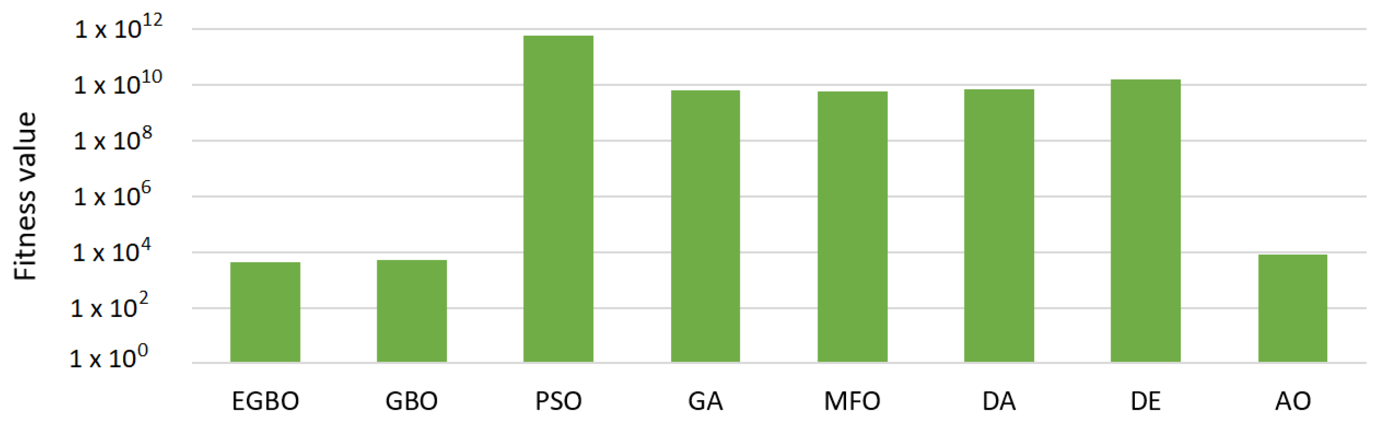
Table 1 tabulates the results of the mean of the fitness function measure. In that table, the proposed EGBO outperformed the other methods in six out of ten functions (i.e., F1–F5, F9); therefore, it was ranked first. The GA was ranked second by obtaining the best values in two functions, F7 and F8. The GBO came in the third rank with the best values in three functions, F1–F3, followed by the MFO. The rest of the algorithms were ordered: the AO, DE, DA, and PSO, respectively. Figure 1 illustrates the average fitness function values for all methods over all functions.

The results of the standard deviation measure are reported in Table 2 to show the stability of each method. In this measure, the smallest value indicates good stability behavior within the independent runs. The results show that the proposed EGBO showed the best stability in 70% of the functions compared to the other methods followed by the DE and GBO. The GA, AO, and MFO came in the fourth, fifth, and sixth ranks.

The results of the max measure are listed in Table 3. In this table, the worst value of each algorithm for each function is recorded. As seen in the table, the worst values of the proposed EGBO were better than the compared methods in six out of ten functions (i.e., F1–F3, F5, and F8–F9). The GA was ranked second by obtaining the best values in both F6 and F10. The MFO and GBO came in the third and fourth ranks, followed by the DE and AO.

Furthermore, the results of the min measure are presented in Table 4. In this measure, the best values so far obtained by each algorithm are recorded. As seen in the results, the proposed EGBO obtained the best values in four out of ten functions (i.e., F1, F2, F5, and F9) and obtained good results in the rest of the functions. The GA ranked second by obtaining the minimum values in F4 and F8 functions. The GBO came in third, followed by the MFO, DA, D, PSO, and AO.

The computation time is also considered in Table 5. In this measure, the MFO algorithm was the fastest among all methods, followed by the PSO and AO. The EGBO consumed an acceptable computation time in each function and was ranked fourth, followed by GBO, GA, and DE. The slower algorithm was the DA; it recorded the longest computation time in each function. Figure 2 illustrates the average computation times for all methods over all functions.

Moreover, Figure 3 illustrates the convergence curves for all methods during the optimization process. From this figure, it can be seen that the proposed EGBO can effectively maintain the populations to converge toward the optimal value as shown in F1, F4, F5, and F9. The PSO, GBO, and MFO also showed second-best convergence. In contrast, the DA algorithm showed the worst convergence in most functions.

Furthermore,

Table 6. Results of the Wilcoxon rank-sum test for global optimization.

	GBO	PSO	GA	MFO	DA	DE	AO
F1	0.0015	0.0000	0.0000	0.0000	0.0000	0.0000	0.0000
F2	0.3506	0.0000	0.0005	0.0000	0.0000	0.0000	0.0000
F3	0.8678	0.9970	0.7878	0.4199	0.2510	0.0622	0.0757
F4	0.0015	0.0000	0.0114	0.0003	0.0000	0.0381	0.0000
F5	0.3085	0.0000	0.6331	0.0003	0.0000	0.0000	0.0000
F6	0.0374	0.0397	0.0000	0.0000	0.0000	0.0004	0.4423
F7	0.8519	0.9338	0.7716	0.4553	0.0251	0.0012	0.0066
F8	0.0321	0.1973	0.0222	0.6776	0.3712	0.0001	0.0020
F9	0.0281	0.0000	0.3093	0.0000	0.0000	0.0536	0.0000
F10	0.6061	0.1360	0.0000	0.0000	0.0000	0.0000	0.2814

Boldface indicates the best result.

records the Wilcoxon rank-sum test as a statistical test to check if there is a statistical difference between the EGBO and the compared algorithms at a p-value < 0.05. The results, as recorded in Table 6, show significant differences between the proposed EGBO and the compared algorithms, especially with MFO, DA, DE, and AO, which indicates the effectiveness of the EGBO in solving global optimization problems.

In light of the above results, the proposed EGBO method can effectively solve global optimization problems and provide promising results compared to the other methods. Therefore, in the next section, it will be evaluated in solving different feature selection problems.

4.2. Second Experiment: Solving Feature Selection Problem

In this part, the proposed EGBO method is assessed in solving different feature selection problems using twelve well-known feature selection datasets from [27];

Table 7. Datasets description.

Datasets	Features	Samples	Classes
Exactly2	13	1000	2
breast cancer	9	699	2
ionosphere	34	351	2
glass	9	214	7
Lymphography	18	148	2
sonar	60	208	2
waveform	40	5000	3
clean1data	166	476	2
tic-tac-toe	9	958	2
heart	12	270	2
SPECT	22	267	2
Zoo	16	101	6

lists their descriptions.

The performance of the proposed method is evaluated by five measures, namely fitness value (Equation (31)), accuracy (Acc) as in Equation (32), standard deviation (Std) as in Equation (30), number of selected features, and the computation time for each algorithm. The results are recorded in

Table 8. Results of the fitness function values.

	EGBO	GBO	PSO	GA	AO	DE	MFO	DA
ionosphere	0.1258	0.1556	0.1327	0.1792	0.2254	0.1388	0.2540	0.2923
breast cancer	0.1530	0.2047	0.1921	0.2131	0.2513	0.1792	0.3010	0.2497
glass	0.1294	0.1379	0.1410	0.1460	0.1749	0.1372	0.2055	0.1502
sonar	0.0533	0.1039	0.0593	0.1693	0.3222	0.0931	0.2954	0.2257
Lymphography	0.2078	0.2723	0.2317	0.3011	0.4578	0.2377	0.4755	0.3284
tic-tac-toe	0.0000	0.0043	0.0043	0.0360	0.0043	0.0043	0.4734	0.0735
waveform	0.6203	0.6360	0.6267	0.6394	0.6571	0.6215	0.6709	0.6558
clean1data	0.1421	0.2108	0.2035	0.2191	0.3043	0.2030	0.2691	0.2689
SPECT	0.3220	0.3549	0.3288	0.3464	0.4036	0.3267	0.4262	0.3753
Zoo	0.0000	0.0022	0.0044	0.0044	0.0373	0.0022	0.1141	0.0067
Exactly2	0.4685	0.4838	0.4855	0.4895	0.5109	0.4793	0.5735	0.5001
heart	0.3321	0.3517	0.3449	0.3588	0.4201	0.3388	0.4496	0.3980

Boldface indicates the best result.

,

Table 9. Results of the standard deviation.

	EGBO	GBO	PSO	GA	AO	DE	MFO	DA
ionosphere	0.0485	0.0619	0.0660	0.0707	0.0868	0.0649	0.0376	0.0408
breast cancer	0.0349	0.0231	0.0416	0.0394	0.0593	0.0443	0.0507	0.0359
glass	0.0219	0.0319	0.0282	0.0348	0.0370	0.0308	0.0430	0.0290
sonar	0.0675	0.0918	0.0739	0.0287	0.1016	0.0894	0.0616	0.0538
Lymphography	0.1042	0.0934	0.1058	0.0696	0.1176	0.0811	0.0902	0.0624
tic-tac-toe	0.0000	0.0161	0.0161	0.0807	0.0161	0.0161	0.0940	0.1257
waveform	0.0123	0.0180	0.0143	0.0126	0.0344	0.0135	0.0301	0.0180
clean1data	0.0144	0.0455	0.0415	0.0358	0.0613	0.0369	0.0394	0.0408
SPECT	0.0284	0.0372	0.0364	0.0371	0.0570	0.0414	0.0668	0.0381
Zoo	0.0000	0.0083	0.0113	0.0113	0.0662	0.0083	0.0879	0.0133
Exactly2	0.0231	0.0251	0.0244	0.0206	0.0376	0.0210	0.0266	0.0175
heart	0.0283	0.0442	0.0415	0.0357	0.0714	0.0388	0.0606	0.0423

Boldface indicates the best result.

,

Table 10. Ratios of the selected features.

	EGBO	GBO	PSO	GA	AO	DE	MFO	DA
ionosphere	0.3309	0.3588	0.4275	0.4275	0.3412	0.4294	0.4745	0.4902
breast cancer	0.3137	0.4275	0.4431	0.4118	0.3294	0.4314	0.4549	0.5059
glass	0.5051	0.5111	0.5185	0.5333	0.6370	0.5111	0.5926	0.5852
sonar	0.4487	0.4811	0.4811	0.4978	0.5511	0.4644	0.5167	0.5011
Lymphography	0.5208	0.5185	0.4926	0.5370	0.5519	0.5148	0.5370	0.5593
tic-tac-toe	0.8068	1.0000	1.0000	0.9852	1.0000	1.0000	0.8194	0.9704
waveform	0.6190	0.6794	0.6794	0.6921	0.7492	0.6667	0.6476	0.6571
clean1data	0.3213	0.4458	0.4940	0.4932	0.4506	0.4928	0.5390	0.5233
SPECT	0.5130	0.4364	0.4727	0.5152	0.5091	0.4515	0.5152	0.5333
Zoo	0.5268	0.5708	0.5833	0.5708	0.6083	0.5833	0.5395	0.6250
Exactly2	0.2212	0.2615	0.4000	0.4205	0.3641	0.4667	0.5026	0.4359
heart	0.5513	0.6058	0.5865	0.6090	0.6090	0.6218	0.5224	0.5692

Boldface indicates the best result.

,

Table 11. Results of the accuracy measure.

	EGBO	GBO	PSO	GA	AO	DE	MFO	DA
ionosphere	0.9818	0.9720	0.9780	0.9629	0.9417	0.9765	0.9341	0.9129
breast cancer	0.9754	0.9576	0.9614	0.9530	0.9333	0.9659	0.9068	0.9364
glass	0.7994	0.7560	0.7497	0.7509	0.6881	0.7484	0.6579	0.7522
sonar	0.9926	0.9808	0.9910	0.9705	0.8859	0.9833	0.9090	0.9462
Lymphography	0.9459	0.9171	0.9351	0.9045	0.7982	0.9369	0.7982	0.8883
tic-tac-toe	1.0000	0.9997	0.9997	0.9922	0.9997	0.9997	0.7671	0.9788
waveform	0.7989	0.7931	0.7970	0.7926	0.7839	0.7981	0.7723	0.7818
clean1data	0.9796	0.9535	0.9569	0.9507	0.9036	0.9574	0.9261	0.9261
SPECT	0.8955	0.8726	0.8905	0.8786	0.8338	0.8915	0.8139	0.8577
Zoo	1.0000	0.9973	0.9947	0.9947	0.9680	0.9973	0.8880	0.9920
Exactly2	0.7800	0.7653	0.7637	0.7600	0.7376	0.7699	0.6704	0.7496
heart	0.8889	0.8744	0.8794	0.8700	0.8184	0.8837	0.7942	0.8398

Boldface indicates the best result.

,

Table 12. Computation times for all algorithms.

	EGBO	GBO	PSO	GA	AO	DE	MFO	DA
ionosphere	25.418	25.479	24.920	28.329	50.309	25.402	24.979	28.792
breast cancer	25.525	25.538	25.012	28.411	50.412	25.487	25.078	26.812
glass	26.260	27.561	26.582	31.291	52.116	27.344	27.201	28.430
sonar	25.158	25.171	24.696	28.141	49.700	25.142	24.777	27.189
Lymphography	21.516	23.066	21.789	26.201	39.414	21.717	22.758	22.909
tic-tac-toe	27.647	29.758	29.271	34.574	58.779	30.435	29.962	30.080
waveform	166.431	157.170	162.899	190.428	314.278	164.305	164.992	151.181
clean1data	30.409	32.733	33.144	37.645	64.316	33.762	33.622	40.541
SPECT	22.077	25.104	25.030	28.644	48.344	25.692	25.174	26.721
Zoo	7.729	26.908	25.383	32.773	49.306	25.945	27.188	26.930
Exactly2	24.346	24.489	27.296	28.711	49.987	29.136	26.953	27.980
heart	25.401	25.479	24.990	28.378	49.885	25.453	25.188	26.242

Boldface indicates the best result.

and

Table 13. Results of the Wilcoxon rank-sum test.

	GBO	PSO	GA	AO	DE	MFO	DA
ionosphere	0.4843	0.0063	0.1001	0.0006	0.0231	0.0000	0.0141
breast cancer	0.2069	0.8077	0.0000	0.0000	0.3432	0.0000	0.0000
glass	0.0127	0.0034	0.0006	0.0000	0.0223	0.0000	0.0000
sonar	0.1639	0.0036	0.0388	0.1639	0.0015	0.0000	0.0185
Lymphography	0.0095	0.0432	0.0003	0.0007	0.7025	0.0000	0.0000
tic-tac-toe	0.0012	0.2245	0.0026	0.0000	0.1609	0.0000	0.0002
waveform	0.1639	0.0798	0.0798	0.0038	0.1639	0.0000	0.0386
clean1data	0.0371	0.3575	0.0021	0.0002	0.1186	0.0000	0.0000
SPECT	0.0000	0.0002	0.0000	0.0000	0.0022	0.0000	0.0000
Zoo	0.0000	0.0000	0.0000	0.0000	0.0000	0.0000	0.0000
Exactly2	0.0017	0.0008	0.0005	0.0001	0.0049	0.0000	0.0000
heart	0.0649	0.2815	0.0345	0.0001	0.6431	0.0000	0.0000

Boldface indicates the best result.

.

$$f\left(x_i\left(t\right)\right)=\xi E_{x_i\left(t\right)}+(1-\xi )\left(\frac{c}{C}\right),$$

(31)

where $E_{x_i\left(t\right)}$ denotes the error value of the classification process (kNN is used in this paper as a classifier). The second term defines the selected feature number. $\xi \in [0,1]$ is used to balance the number of the selected features and the classification error. c and C are the current and ’all-feature’ numbers, respectively.

$$Accuracy\left(Acc\right)=\frac{TP1+TN1}{TP1+TN1+FP1+FN1}$$

(32)

where the number of positive classes correctly classified is ($TP1$), whereas the number of negative classes correctly classified is ($TN1$). Both $FP1$ and $FN1$ are the numbers of positive and negative classes incorrectly classified, respectively.

Table 8 shows the results of the fitness function values for all algorithms over all datasets. These results indicate that the proposed EGBO obtained the best fitness value among the compared algorithms and performed well in all datasets. The DE obtained the second-best results in 75% of the datasets. The PSO came in third, followed by GBO, GA, DA, AO, and MFO. Figure 4 illustrates the average of this measure over all datasets, which shows that the EGBO obtained the smallest average among all methods.

The stability results of all algorithms are listed in Table 9. As in that table, the proposed EGBO showed the most stable algorithm in 7 out of 12 datasets: glass, tic-tac-toe, waveform, clean1data, SPECT, Zoo, and heart. The GA and DE ranked second and third for stability, respectively, followed by PSO, DA, and GBO.

As mentioned above, this experiment aims to decrease each dataset’s features by deleting the redundant descriptors and keeping the best ones. Therefore, Table 10 reports the number of selected features in each dataset. From Table 10, we can see that the EGBO chose the smallest number of features in 9 out of 12 datasets and showed good performance in the remaining datasets. The GBO was ranked second, followed by MFO, AO, DE, PSO, and GA. In this regard, the small number of features is sometimes the best; therefore, we used the classification accuracy measure to evaluate the obtained feature by each algorithm.

Consequently, the classification accuracy measure was used to evaluate the proposed method’s ability to classify the samples of each dataset correctly. The results of this measure were recorded in Table 11. This table shows that the EGBO ranked first; it outperformed the other methods and obtained high-accuracy results in all datasets. The DE came in the second rank, whereas the PSO obtained the third, followed by the GBO, GA, DA, and AO. In contrast, the MFO recorded the worst accuracy measures in most datasets.

The computation times for all methods were also measured. Table 12 records the time consumed by each algorithm. By analyzing the results, we can note that all algorithms consumed similar times to some extent. In detail, the EGBO was the fastest in 59% of the datasets, followed by PSO, MFO, DE, GBO, and DA, respectively, whereas the GA and AO recorded the longest computation time.

Furthermore, an example of the convergence curves for all methods is illustrated in Figure 5. In this figure, a sample of the datasets is presented, which shows that the proposed EGBO method converged to the optimal values faster than the compared algorithms, which indicates the good convergence behaviors of the EGBO when solving feature selection problems.

In addition, Table 13 shows the Wilcoxon rank-sum test as a statistical test to check if there is a statistical difference between the proposed method and the other algorithms at a p-value < 0.05. From this table, we can see that there are significant differences between the proposed methods and the other algorithms in most datasets, indicating the EGBO’s effectiveness in solving different feature selection problems.

From the previous results, the proposed EGBO method outperformed the compared algorithms in most cases in solving global optimization problems and selecting the most relative features. These promising results can be attributed to a few reasons, e.g., the local escaping operator of the GBO was extended to include the expanded and narrowed exploration behavior, which added more flexibility and reliability to the traditional GBO algorithm. This extension increased the ability of the GBO to explore more areas in the search space, reflecting on effectively reaching the optimal point. On the other hand, although the EGBO obtained good results in most cases, it failed to show the best results in the computation time measure, namely in the global optimization experiment. This defect can be due to the traditional GBO consuming a relatively longer time than the compared algorithm when performing an optimization task. Therefore, this defect can be studied in future work. Generally, the exploration behaviors used in the EGBO increased the performance of the traditional algorithm in terms of performance measures.

5. Conclusions

This paper proposed a new version of the gradient-based optimizer (GBO), called EGBO, to solve diverse optimization problems, namely global optimization and feature selection. The local search of the EGBO was improved and expanded using expanded and narrowed exploration behaviors to increase the ability of the GBO to explore broad areas in the search space. The effectiveness of the EGBO was checked and evaluated using CEC2019 as global optimization functions and twelve benchmark feature selection datasets. The results were analyzed and compared to a set of well-known optimization algorithms using six performance measures. The EGBO showed promising results in solving global optimization problems, recording the highlight accuracy, selecting the most significant features, and outperforming the compared methods and the traditional version of the GBO in terms of performance measures. However, the computation time of the EGBO needs to be improved. In future works, the EGBO will be evaluated and applied in parameter estimation, image segmentation, and classifier optimization. In addition, the complexity of the EGBO will be maintained, and its initial population will be improved using chaotic maps to add more diversity to the search space.

References

1. Tubishat, M.; Ja’afar, S.; Alswaitti, M.; Mirjalili, S.; Idris, N.; Ismail, M.A.; Omar, M.S. Dynamic salp swarm algorithm for feature selection. Expert Syst. Appl. 2021, 164, 113873. [Google Scholar] [CrossRef]
2. Ewees, A.A.; ElLaban, H.A.; ElEraky, R.M. Features selection for facial expression recognition. In Proceedings of the 2019 10th International Conference on Computing, Communication and Networking Technologies (ICCCNT), Kanpur, India, 6–8 July 2019; pp. 1–6. [Google Scholar]
3. Huda, R.K.; Banka, H. Efficient feature selection methods using PSO with fuzzy rough set as fitness function. Soft Comput. 2022, 26, 2501–2521. [Google Scholar] [CrossRef]
4. Gaheen, M.M.; ElEraky, R.M.; Ewees, A.A. Automated students arabic essay scoring using trained neural network by e-jaya optimization to support personalized system of instruction. Educ. Inf. Technol. 2021, 26, 1165–1181. [Google Scholar] [CrossRef]
5. Ewees, A.A.; Al-qaness, M.A.; Abualigah, L.; Oliva, D.; Algamal, Z.Y.; Anter, A.M.; Ali Ibrahim, R.; Ghoniem, R.M.; Abd Elaziz, M. Boosting Arithmetic Optimization Algorithm with Genetic Algorithm Operators for Feature Selection: Case Study on Cox Proportional Hazards Model. Mathematics 2021, 9, 2321. [Google Scholar] [CrossRef]
6. Nadimi-Shahraki, M.H.; Zamani, H.; Mirjalili, S. Enhanced whale optimization algorithm for medical feature selection: A COVID-19 case study. Comput. Biol. Med. 2022, 148, 105858. [Google Scholar] [CrossRef]
7. Zhang, Y.; Liu, R.; Wang, X.; Chen, H.; Li, C. Boosted binary Harris hawks optimizer and feature selection. Eng. Comput. 2021, 37, 3741–3770. [Google Scholar] [CrossRef]
8. Banerjee, D.; Chatterjee, B.; Bhowal, P.; Bhattacharyya, T.; Malakar, S.; Sarkar, R. A new wrapper feature selection method for language-invariant offline signature verification. Expert Syst. Appl. 2021, 186, 115756. [Google Scholar] [CrossRef]
9. Sathiyabhama, B.; Kumar, S.U.; Jayanthi, J.; Sathiya, T.; Ilavarasi, A.; Yuvarajan, V.; Gopikrishna, K. A novel feature selection framework based on grey wolf optimizer for mammogram image analysis. Neural Comput. Appl. 2021, 33, 14583–14602. [Google Scholar] [CrossRef]
10. Ewees, A.A.; Ismail, F.H.; Ghoniem, R.M. Wild Horse Optimizer-Based Spiral Updating for Feature Selection. IEEE Access 2022, 10, 106258–106274. [Google Scholar] [CrossRef]
11. Bandyopadhyay, R.; Basu, A.; Cuevas, E.; Sarkar, R. Harris Hawks optimisation with Simulated Annealing as a deep feature selection method for screening of COVID-19 CT-scans. Appl. Soft Comput. 2021, 111, 107698. [Google Scholar] [CrossRef]
12. Abualigah, L.; Yousri, D.; Abd Elaziz, M.; Ewees, A.A.; Al-qaness, M.A.; Gandomi, A.H. Aquila Optimizer: A novel meta-heuristic optimization Algorithm. Comput. Ind. Eng. 2021, 157, 107250. [Google Scholar] [CrossRef]
13. Ahmadianfar, I.; Bozorg-Haddad, O.; Chu, X. Gradient-based optimizer: A new metaheuristic optimization algorithm. Inf. Sci. 2020, 540, 131–159. [Google Scholar] [CrossRef]
14. Ahmadianfar, I.; Gong, W.; Heidari, A.A.; Golilarz, N.A.; Samadi-Koucheksaraee, A.; Chen, H. Gradient-based optimization with ranking mechanisms for parameter identification of photovoltaic systems. Energy Rep. 2021, 7, 3979–3997. [Google Scholar] [CrossRef]
15. Khalilpourazari, S.; Doulabi, H.H.; Çiftçioğlu, A.Ö.; Weber, G.W. Gradient-based grey wolf optimizer with Gaussian walk: Application in modelling and prediction of the COVID-19 pandemic. Expert Syst. Appl. 2021, 177, 114920. [Google Scholar] [CrossRef] [PubMed]
16. AlRassas, A.M.; Al-qaness, M.A.; Ewees, A.A.; Ren, S.; Abd Elaziz, M.; Damaševičius, R.; Krilavičius, T. Optimized ANFIS model using Aquila Optimizer for oil production forecasting. Processes 2021, 9, 1194. [Google Scholar] [CrossRef]
17. Ma, L.; Li, J.; Zhao, Y. Population Forecast of China’s Rural Community Based on CFANGBM and Improved Aquila Optimizer Algorithm. Fractal Fract. 2021, 5, 190. [Google Scholar] [CrossRef]
18. Zhou, W.; Wang, P.; Heidari, A.A.; Zhao, X.; Turabieh, H.; Chen, H. Random learning gradient based optimization for efficient design of photovoltaic models. Energy Convers. Manag. 2021, 230, 113751. [Google Scholar] [CrossRef]
19. Jiang, Y.; Luo, Q.; Zhou, Y. Improved gradient-based optimizer for parameters extraction of photovoltaic models. IET Renew. Power Gener. 2022, 16, 1602–1622. [Google Scholar] [CrossRef]
20. Ewees, A.A.; Ismail, F.H.; Sahlol, A.T. Gradient-based optimizer improved by Slime Mould Algorithm for global optimization and feature selection for diverse computation problems. Expert Syst. Appl. 2023, 213, 118872. [Google Scholar] [CrossRef]
21. Kennedy, J.; Eberhart, R. Particle swarm optimization. In Proceedings of the ICNN’95-International Conference on Neural Networks, Perth, WA, Australia, 27 November–1 December 1995; Volume 4, pp. 1942–1948. [Google Scholar]
22. Mitchell, M. An Introduction to Genetic Algorithms; MIT Press: Cambridge, MA, USA, 1998. [Google Scholar]
23. Storn, R.; Price, K. Differential evolution—A simple and efficient heuristic for global optimization over continuous spaces. J. Glob. Optim. 1997, 11, 341–359. [Google Scholar] [CrossRef]
24. Mirjalili, S. Dragonfly algorithm: A new meta-heuristic optimization technique for solving single-objective, discrete, and multi-objective problems. Neural Comput. Appl. 2016, 27, 1053–1073. [Google Scholar] [CrossRef]
25. Mirjalili, S. Moth-flame optimization algorithm: A novel nature-inspired heuristic paradigm. Knowl.-Based Syst. 2015, 89, 228–249. [Google Scholar] [CrossRef]
26. Price, K.; Awad, N.; Ali, M.; Suganthan, P. Problem definitions and evaluation criteria for the 100-digit challenge special session and competition on single objective numerical optimization. In Technical Report; Nanyang Technological University: Singapore, 2018. [Google Scholar]
27. Dua, D.; Graff, C. UCI Machine Learning Repository, 2019; University of California, Irvine, School of Information and Computer Sciences: Irvine, CA, USA, 2019. [Google Scholar]
Figure 1. Average fitness function values for all methods in all functions.
Mathematics 11 00378 g001
Figure 2. Average computation times for all methods in all functions.
Mathematics 11 00378 g002
Figure 3. Convergence curves for the proposed EGBO and the compared methods.
Mathematics 11 00378 g003
Figure 4. Average of the fitness function values for all methods.
Mathematics 11 00378 g004
Figure 5. Example of the convergence curves for the proposed EGBO and the compared methods.
Mathematics 11 00378 g005