New Modified Couple Stress Theory of Thermoelasticity with Hyperbolic Two Temperature

Abstract

This paper deals with the two-dimensional deformation in fibre-reinforced composites with new modified couple stress thermoelastic theory (nMCST) due to concentrated inclined load. Lord Shulman heat conduction equation with hyperbolic two temperature (H2T) has been used to form the mathematical model. Fourier and Laplace transform are used for obtaining the physical quantities of the mathematical model. The expressions for displacement components, thermodynamic temperature, conductive temperature, axial stress, tangential stress and couple stress are obtained in the transformed domain. A mathematical inversion procedure has been used to obtain the inversion of the integral transforms using MATLAB software. The effects of hyperbolic and classical two temperature are shown realistically on the various physical quantities.

1. Introduction

Low weight and high strength make fibre-reinforced composites an ideal material for many structures. The mechanical properties of such materials can be explained using a continuum model. Manmade fibre-reinforced composites are proving to be particularly effective in this regard. The materials (natural and synthetic) in which the properties like thermal conductivity vary with orientation are called anisotropic materials. For example, crystals, sedimentary rocks, metals with heavy cold pressing, laminated sheets and heat shielding materials used for space vehicles, wood, cables, fibre-reinforced composite structures, etc. are anisotropic materials. By introducing strong reinforcement fibers in one or more particular directions into a relatively weak, isotropic matrix, a matrix with certain desirable properties is strengthened throughout. An elastic solid reinforced with parallel fibers is usually assumed to be transversely isotropic. Additionally, the response of these composites is typically highly anisotropic, therefore isotropic theory would not be able to accurately predict their behavior under the majority of loading scenarios. For linear constitutive relations, there are five material constants relating to infinitesimal components of stress and strain. For the last three decades, solid mechanics has been studying stress and deformation in fibre-reinforced composite materials.

A revolutionary work was done on fibre-reinforced composite materials by Pipkin and Rogers [1]. Spencer [2] described the deformations of fibre-reinforced materials. Pipkin [3] studied the ideal fiber-reinforced materials that exhibit generalized plane deformations. Testa and Bolay [4] discussed the two key issues with fiber-reinforced materials’ thermoelastic behavior. The maximum stress in each phase of the composite as well as boundaries for the stress at every point in a beam are created in the first. The second issue takes into account the buckling of reinforcing fibres when subjected to thermal loading. The deformations of an idealized incompressible fiber-reinforced material in the finite plane are obtained by Craig and Hart [5]. A revolutionary work was done on fibre-reinforced composite materials by Rogers [6]. Bayones and Hussein [7] studied an anisotropic semi-infinite solid media with fiber-reinforced generalized thermoplastic with respect to thermal relaxation time and gravity effects. Said [8] investigated the effect of hydrostatic initial stress and the gravity field on a fibre-reinforced thermoelastic medium due to its own heat and constant motion using the three-phase-lag model (TPL) and GN theory of thermoelasticity of Type-II.

A macro-scale analysis of materials can be made with the help of classical continuum mechanics theory, which ignores the microstructure size-dependency. For a more complete continuum theory, new deformation measures are needed. This implies that couple stresses must also be introduced into such a theory. Firstly, in 1887, Voigt [9] proposed the asymmetric theory of elasticity, and afterward in 1909, a couple stress theory was presented by Cosserat and Cosserat [10], but examiners deemed the theory not important due to its failure to establish the constitutive interactions. A standard couple stress theory with constitutive relations $t_{ij}=\lambda e_{kk}{\delta }_{ij}+2G{e}_{ij}$, $m_{ij}=4l^{2}G{\chi }_{ij}$ was introduced by Mindlin [11] for isotropic elastic materials. In this theory, Mindlin [11] used a single length scale parameter (LSP). Moreover, the strain tensor in Mindlin’s theory is represented as $e_{ij}=\frac{1}{2}\left(u_{i,j}+u_{j,i}\right)$, and curvature tensors is ${\chi }_{ij}={\omega }_{i,j}$, where the rotation vector is given by ${\omega }_i=\frac{1}{2}{ϵ}_{ijk}{u}_{k,j}$. Due to the asymmetric nature of the couple and curvature stress tensors, this theory is also designated as asymmetric couple stress theory. In addition, Koiter [12] introduced constitutive relationships for anisotropic materials based on Cosserat couple stress theory as $t_{ij}=c_{ijkl}{e}_{kl}$; $m_{ij}=l_i^2{G}_i{\chi }_{ij}$, where $l_i$ $\left(i=1,2,3\right)$ is LSP. Here, $t_{ij}$ is a symmetric tensor, and $m_{ij}$ is an asymmetric tensor. Yang et al. [13] presented a modified couple stress theory (MCST) for isotropic elastic materials with an additional LSP as $t_{ij}=\lambda e_{kk}{\delta }_{ij}+2G{e}_{ij}, m_{ij}=4l^{2}G{\chi }_{ij}$ and $e_{ij}=\frac{1}{2}\left(u_{i,j}+u_{j,i}\right)$, ${\chi }_{ij}=\frac{1}{2}\left({\omega }_{i,j}+{\omega }_{j,i}\right)$, and all the tensors are symmetric. MCST should be extended from isotropic to anisotropic media due to the importance of anisotropic mediums in microstructures. Hence, Chen et al. [14] proposed an nMCST that considers three length-scale parameters for anisotropic materials as

$$t_{ij}=c_{ijkl}{e}_{kl},$$

$$m_{ij}=l_i^2{G}_i{\chi }_{ij}+l_j^2{G}_j{\chi }_{ji},$$

$${\chi }_{ij}={\omega }_{i,j},$$

$${\omega }_i=\frac{1}{2}{ϵ}_{ijk}{u}_{k,j},$$

$$e_{ij}=\frac{1}{2}\left(u_{i,j}+u_{j,i}\right).$$

Here, the ${\chi }_{ij}$ is asymmetric, but the $m_{ij},t_{ij},e_{ij}$ are symmetric tensors.

Chen and Gurtin [4] and Chen et al. [5,6] gave the two-temperature theory of thermoelasticity of deformable bodies for heat conduction, subject to two kinds of temperatures: The thermodynamic temperature $T$ and the conductive temperature $\phi$. According to this theory, we have:

$$T=\phi -b_{ij}{\phi }_{,ij}.$$

For the time-independent cases, the difference between $T$ and $\phi$ is proportional to the supply of heat, and in the absence of heat supply, these temperatures are equal. For time dependent problems, the difference in two temperatures is non zero and does not depend on heat supply. When the two-temperature factor is zero, i.e., $\phi =T$ and then the coupled thermoelasticity can be derived from the two-temperature theory of thermoelasticity. Youssef [15] proved uniqueness theorem for a homogeneous and isotropic media with two temperature generalized thermoelasticity. Youssef [16] proposed a two-temperature model without energy dissipation for an elastic half-space subjected to moving heat source and Youssef [17] constructed a fractional order generalized theory of thermoelasticity based on Duhamel-Neumann stress–strain relation in the context of one temperature and two-temperature. The classical two temperature theory of thermoelasticity, however, does not introduce finite speed of the thermal wave propagation, which is physically unacceptable. Youssef and El Bary [18] improved two temperature theory of thermoelasticity and introduced hyperbolic two temperatures (H2T) theory of thermoelasticity for an isotropic body and proved uniqueness and derived its variational principle and showed finite speed of thermal and mechanical wave propagation. According to this theory, we have:

$$\ddot{\phi }-\ddot{T}=b_{ij}{\phi }_{,ij}$$

Regardless of this, numerous investigators, such as Kaur et al. [19,20], Craciun et al. [21], Khan et al. [22], Marin and Öchsner [23], Singh et al. [24], Zhang et al. [25], Singh et al. [26], Marin et al. [27], Bhatti et al. [28,29,30], Golewski [31,32,33], and Kaur et al. [34,35] worked on various thermoelastic problems. However, until now, no efforts have been made to study the fiber-reinforced thermoelastic medium using nMCST for H2T.

In the present investigation, the two-dimensional deformation in fibre-reinforced composites with nMCST and H2T due to concentrated inclined load and L-S thermoelasticity has been investigated. Laplace and Fourier transform methods are used for obtaining the solutions of the mathematical model. The expressions for displacement components, thermodynamic temperature, conductive temperature, axial stress, tangential stress and couple stress are obtained in the transformed domain. The effects of hyperbolic and classical 2T are illustrated graphically on the various physical quantities.

2. Basic Equations

Following Chen and Li [14], Kumar et al. [36] and Youssef and El Bary [18], the field equations for fibre-reinforced thermoelastic medium with respect to a preferred direction $a_i=\left(a_1,a_2,a_3\right)$, where $a_1^2+a_2^2+a_3^2=1,$ with nMCST and L-S theory of Thermoelasticity with H2T are given by the following equations:

1.

Constitutive Relations

$$t_{ij}=c_{ijkl}{e}_{kl}-{\gamma }_{ij}T,$$

(1)

For fibre reinforced material with respect to a preferred direction $a_i=\left(a_1,a_2,a_3\right)$, where $a_1^2+a_2^2+a_3^2=1,$ we have $c_{ijkl}{e}_{kl}$ in Equation (1), as mentioned below:

$$\begin{array}{cc}\hfill c_{ijkl}{e}_{kl}& =\lambda e_{kk}{\delta }_{ij}+2{\mu }_T{e}_{ij}+\alpha \left(a_k{a}_m{e}_{km}{\delta }_{ij}+a_i{a}_j{e}_{kk}\right)\hfill \\ & +2\left({\mu }_L-{\mu }_T\right)\left(a_i{a}_k{e}_{kj}+a_j{a}_k{e}_{ki}\right)+\beta a_k{a}_m{e}_{km}{a}_i{a}_j\hfill \end{array}$$

$$m_{ij}=l_i^2{G}_i{\chi }_{ij}+l_j^2{G}_j{\chi }_{ji},$$

(2)

$$e_{ij}=\frac{1}{2}(u_{i,j}+u_{j,i}),$$

(3)

$${\chi }_{ij}={\omega }_{i,j},$$

(4)

$${\omega }_i=\frac{1}{2}{ϵ}_{ijk}{u}_{k,j}.$$

(5)

$$\ddot{\phi }-\ddot{T}=b_{ij}{\phi }_{,ij},$$

(6)

$${\gamma }_{ij}=c_{ijkl}{\alpha }_{kl},$$

(7)

2.

Equation of Motion

$$\begin{array}{c}{\left(\lambda e_{kk}{\delta }_{ij}+2{\mu }_T{e}_{ij}+\alpha \left(a_k{a}_m{e}_{km}{\delta }_{ij}+a_i{a}_j{e}_{kk}\right)+2\left({\mu }_L-{\mu }_T\right)\left(a_i{a}_k{e}_{kj}+a_j{a}_k{e}_{ki}\right)+\beta a_k{a}_m{e}_{km}{a}_i{a}_j\right)}_{,j}\\ +\frac{1}{4}\left(l_k^2{G}_k\left({\delta }_{im}{\delta }_{jn}-{\delta }_{in}{\delta }_{jm}\right)u_{n,mllj}+l_l^2{G}_l{ϵ}_{ijk}{u}_{n,mklj}\right)-{\gamma }_{ij}{T}_{,j}=\rho {\ddot{u}}_i, \end{array}$$

(8)

3.

Heat Conduction Equation Proposed by Youssef [15]

$$K_{ij}{\phi }_{,ii}=\left(\frac{\partial }{\partial t}+{\tau }_0\frac{{\partial }^2}{\partial t^2}\right)\left(\rho C_{E}T+{\gamma }_{ij}{T}_0{e}_{ij}\right),$$

(9)

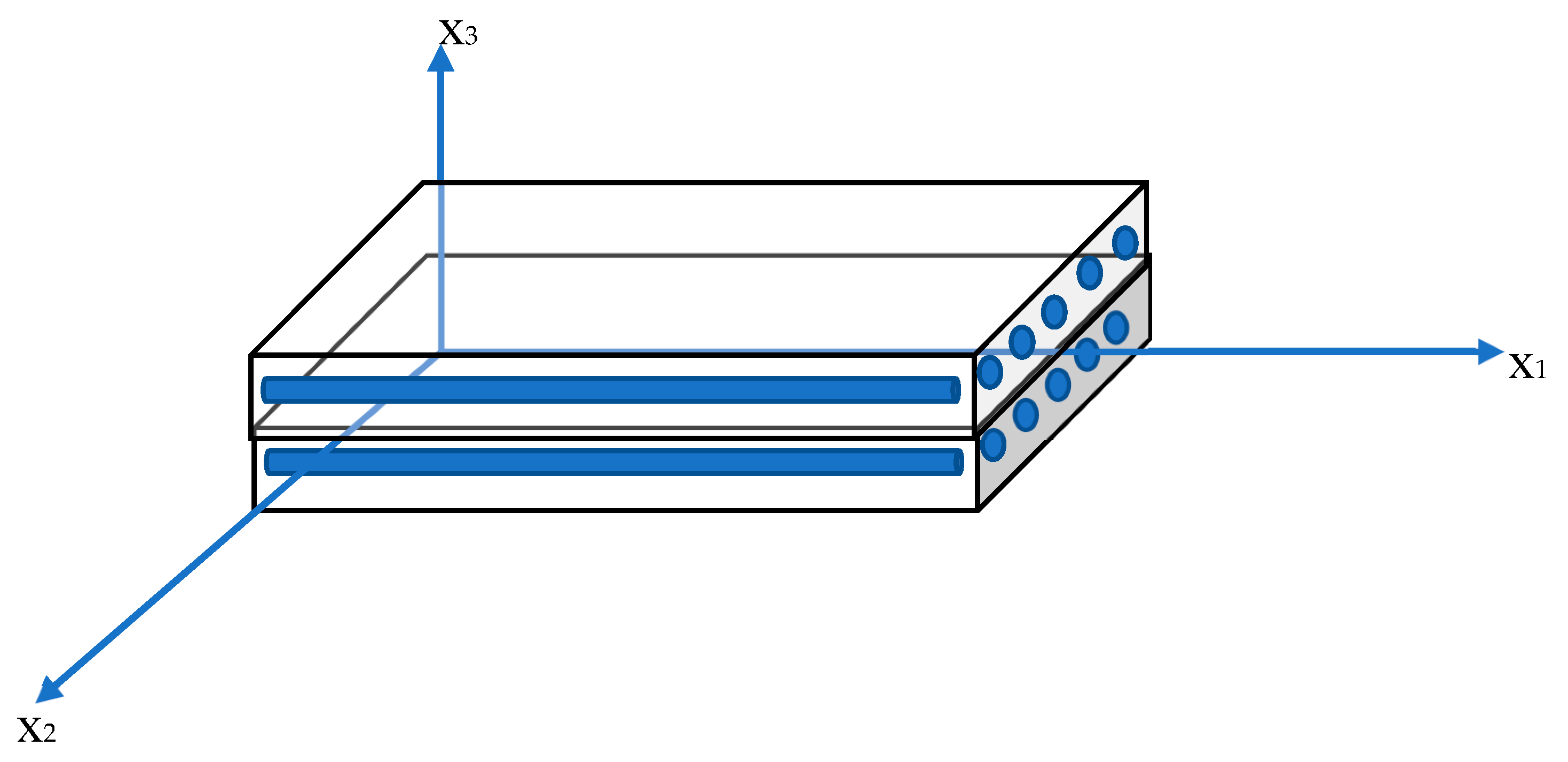
3. Formulation and Solution of the Problem

Consider a 2-D homogeneous fiber-reinforced thermoelastic medium (Figure 1) in the half-space $x_3\ge 0,$ primarily at a uniform temp $T_0.$ We choose the fiber reinforcement direction as $\overrightarrow{a}=\left(0,0,1\right)$ i.e., along $z-$ axis. The rectangular coordinate system ($x_1,x_2,x_3)$ with the origin on the surface $x_2=0$ is considered.

Consider plane strain problem parallel to $x_1{x}_3$ -plane with displacement vector $u=\left(u_1,0,u_3\right)\left(x_1,0,x_3\right)$. The field equations become.

$$\begin{array}{c}\left(\lambda +2{\mu }_T\right)\frac{{\partial }^2{u}_1}{\partial x_1^2}+\left({\mu }_L-\frac{1}{4}{l}_2^2{G}_2\left(\frac{{\partial }^2}{\partial x_1^2}+\frac{{\partial }^2}{\partial x_3^2}\right)\right)\frac{{\partial }^2{u}_1}{\partial x_3^2}\\ +\left(\lambda +\alpha +{\mu }_L+\frac{1}{4}{l}_2^2{G}_2\left(\frac{{\partial }^2}{\partial x_1^2}+\frac{{\partial }^2}{\partial x_3^2}\right)\right)\frac{{\partial }^2{u}_3}{\partial x_1\partial x_3}-{\gamma }_{13}\frac{\partial T}{\partial x_1}=\rho \frac{{\partial }^2{u}_1}{\partial t^2},\end{array}$$

(10)

$$\begin{array}{c}\left(\lambda +4{\mu }_L-2{\mu }_T+2\alpha +\beta \right)\frac{{\partial }^2{u}_3}{\partial x_3^2}+\left({\mu }_L+\lambda +\alpha +\frac{1}{4}{l}_2^2{G}_2\left(\frac{{\partial }^2}{\partial x_1^2}+\frac{{\partial }^2}{\partial x_3^2}\right)\right)\frac{{\partial }^2{u}_1}{\partial x_1\partial x_3}\\ +\left({\mu }_L-\frac{1}{4}{l}_2^2{G}_2\left(\frac{{\partial }^2}{\partial x_1^2}+\frac{{\partial }^2}{\partial x_3^2}\right)\right)\frac{{\partial }^2{u}_3}{\partial x_1^2}-{\gamma }_3\frac{\partial T}{\partial x_3}=\rho \frac{{\partial }^2{u}_3}{\partial t^2},\end{array}$$

(11)

$$K_1\frac{{\partial }^2\phi }{\partial x_1^2}+K_3\frac{{\partial }^2\phi }{\partial x_3^2}-\rho c_E\left(\frac{\partial }{\partial t}+{\tau }_0\frac{{\partial }^2}{\partial t^2}\right)T=T_0\left(\frac{\partial }{\partial t}+{\tau }_0\frac{{\partial }^2}{\partial t^2}\right)\left({\gamma }_1\frac{\partial u_1}{\partial x_1}+{\gamma }_3\frac{\partial u_3}{\partial x_3}\right),$$

(12)

$$\frac{{\partial }^{2}T}{\partial t^2}=\frac{{\partial }^2\phi }{\partial t^2}-b_1\frac{{\partial }^2\phi }{\partial x_1^2}-b_3\frac{{\partial }^2\phi }{\partial x_3^2}.$$

(13)

where $c_{11}=c_{22}=\left(\lambda +2{\mu }_T\right),c_{23}=c_{13}=\left(\lambda +\alpha \right),c_{33}=\left(\lambda +4{\mu }_L-2{\mu }_T+2\alpha +\beta \right),c_{66}=\frac{c_{11}-c_{12}}{2}={\mu }_T,c_{55}=c_{44}={\mu }_L,c_{12}=\lambda ,$ we have used the notations $11\to 1,22\to 2,33\to 3,23\to 4,13\to 5,12\to 6$ for the material constants.

${\gamma }_1=\left(\lambda +2{\mu }_T+\lambda \right){\alpha }_1+\left(\lambda +\alpha \right){\alpha }_3$, ${\gamma }_3=2\left(\lambda +\alpha \right){\alpha }_1+\left(\lambda +4{\mu }_L-2{\mu }_T+2\alpha +\beta \right){\alpha }_3.$ Additionally, the stress components and couple stress are

$$t_{33}=\left(\lambda +\alpha \right)\frac{\partial u_1}{\partial x_1}+\left(\lambda +4{\mu }_L-2{\mu }_T+2\alpha +\beta \right)\frac{\partial u_3}{\partial x_3}-{\gamma }_{3}T,$$

(14)

$$t_{31}={\mu }_L\left(\frac{\partial u_1}{\partial x_3}+\frac{\partial u_3}{\partial x_1}\right),$$

(15)

$$m_{32}=m_{23}=\frac{1}{2}{l}_2^2{G}_2\left(\frac{{\partial }^2{u}_1}{\partial x_3^2}-\frac{{\partial }^2{u}_3}{\partial x_1\partial x_3}\right),$$

(16)

$$m_{12}=m_{21}=\frac{1}{2}{l}_2^2{G}_2\left(\frac{{\partial }^2{u}_1}{\partial x_1\partial x_3}-\frac{{\partial }^2{u}_3}{\partial x_1^2}\right),$$

(17)

$$m_{11}=m_{13}=m_{22}=m_{31}=m_{33}=0$$

(18)

The preliminary and regularity conditions are given by

$$u_1\left(x_1, x_3, 0\right)=0=\dot{u_1} \left(x_1, x_3, 0\right)$$

(19)

$$u_3\left(x_1, x_3, 0\right)=0=\dot{u_3} \left(x_1, x_3, 0\right)$$

(20)

$$T\left(x_1, x_3, 0\right)=0=\dot{T}\left(x_1, x_3, 0\right)$$

(21)

$$\phi \left(x_1, x_3, 0\right)=0=\dot{\phi }\left(x_1, x_3, 0\right) for x_3\ge 0,-\infty <x_1<\infty$$

(22)

$$u_1\left(x_1, x_3, t\right)=u_3\left(x_1, x_3, t\right)=T\left(x_1, x_3, 0\right)=\phi \left(x_1, x_3, 0\right)=0 \mathrm{for} t>0 \mathit{when} x_3\to \infty$$

(23)

Dimensionless quantities are given by

$$\begin{array}{c}{x}_1^{\prime }=\frac{x_1}{L},x_3^{\prime }=\frac{x_3}{L},u_1^{\prime }=\frac{\rho c_1^2}{L{\gamma }_1{T}_0}{u}_1,u_3^{\prime }=\frac{\rho c_1^2}{L{\gamma }_1{T}_0}{u}_3,T^{\prime }=\frac{T}{T_0},{\phi }^{\prime }=\frac{\phi }{T_0} t^{\prime }=\frac{c_1}{L}t,t_{11}^{\prime }=\frac{t_{11}}{{\gamma }_1{T}_0},t_{33}^{\prime }=\frac{t_{33}}{{\gamma }_1{T}_0},\\ m_{32}^{\prime }=\frac{m_{32}}{L{\gamma }_1{T}_0},l_i^{\prime }=\frac{l_i}{L},G_i^{\prime }=\frac{G_i}{\rho c_1^2},c_1^2=\frac{\left(\lambda +2{\mu }_T\right)}{\rho }\end{array}$$

(24)

The Laplace transforms is defined by

$$\mathcal{L}\left[f\left(x_1, x_3,t\right)\right]=\underset{0}{\overset{\infty }{{\displaystyle \int }}}{e}^{-st}f\left(x_1, x_3,t\right)dt=\tilde{f}\left(x_1, x_3,s\right)$$

(25)

with basic properties

$$L\left(\frac{\partial f}{\partial t}\right)=s\overline{f}\left(x_1, x_3,s\right)-f\left(x_1, x_3,0\right),$$

(26)

$$L\left(\frac{{\partial }^{2}f}{\partial t^2}\right)=s^2\overline{f}\left(x_1, x_3,s\right)-sf\left(x_1, x_3,0\right)-{\left(\frac{\partial f}{\partial t}\right)}_{t=0}.$$

(27)

Fourier transforms of a function $\overline{f}$ w.r.t. variable $x$ with $\xi$ as a Fourier variable is

$$\widehat{f}\left(\xi ,x_3,s\right)=\underset{-\infty }{\overset{\infty }{{\displaystyle \int }}}\overline{f}\left(x_1, x_3,s\right)e^{i\xi x_1}d{x}_1.$$

(28)

Such that if $f\left(x_1\right)\to 0$ and $f^{n-1}\left(x_1\right)\to 0,$ as $x_1\to \pm \infty ,$ then

$$\mathcal{F}\left\{\frac{{\partial }^{n}f\left(x_1, x_3,s\right)}{\partial x_1^n}\right\}={\left(i\xi \right)}^n\widehat{f}\left(\xi ,x_3,s\right).$$

(29)

Using the dimensionless quantities defined by (17) into Equations (10)–(16) and suppressing the primes, the Equations (9)–(14) and then applying Laplace and Fourier transform defined by (25) and (28) becomes

$$\left({\zeta }_1+{\zeta }_2{D}^2+{\zeta }_3{D}^4\right)\widehat{u}+\left({\zeta }_{4}D+{\zeta }_5{D}^3\right)\widehat{w}+{\zeta }_6\widehat{T}=0,$$

(30)

$$\left({\zeta }_{4}D+{\zeta }_5{D}^3\right)\widehat{u}+\left({\zeta }_7+{\zeta }_8{D}^2\right)\widehat{w}+{\zeta }_{9}D\widehat{T}=0,$$

(31)

$${\zeta }_{10}\widehat{u}+{\zeta }_{11}D\widehat{w}+{\zeta }_{12}\widehat{T}+\left({\zeta }_{13}+{\delta }_3{D}^2\right)\widehat{\phi }=0,$$

(32)

$$\left({\zeta }_{14}-{\zeta }_{15}{D}^2\right)\widehat{\phi }+{\zeta }_{16}\widehat{T}=0,$$

(33)

$${\widehat{t}}_{33}={\zeta }_{17}\widehat{u}+{\delta }_{4}D\widehat{w}+{\zeta }_9\widehat{T},$$

(34)

$${\widehat{t}}_{31}={\delta }_{1}D\widehat{u}+{\zeta }_{18}\widehat{w},$$

(35)

$$m_{32}=-2\left({\zeta }_3{D}^2\widehat{u}+{\zeta }_5\widehat{w}\right).$$

(36)

where

$$\begin{array}{c}{\delta }_1=\frac{{\mu }_L}{\rho c_1^2}, {\delta }_2=\frac{\left(\lambda +\alpha +{\mu }_L\right)}{\rho c_1^2}, {\delta }_4=\frac{\left(\lambda +4{\mu }_L-2{\mu }_T+2\alpha +\beta \right)}{\rho c_1^2}, {\delta }_3=\frac{-K_3}{K_1}, {\delta }_5=\frac{\rho C_{\mathrm{E}}{C}_{1}L}{K_1}\left(s+\frac{{\tau }_0{C}_1{s}^2}{L}\right),\\ {\delta }_6=\frac{L{T}_0{\gamma }_1}{\rho C_1{K}_1}\left(s+\frac{{\tau }_0{C}_1{s}^2}{L}\right), {\delta }_8=\frac{\left(\lambda +\alpha \right)}{\rho c_1^2}, {\zeta }_1=-{\xi }^2-s^2, {\mathsf{\zeta }}_2={\delta }_1+\frac{1}{4}{l}_2^2{G}_2{\xi }^2,\\ {\mathsf{\zeta }}_3=-\frac{1}{4}\left(l_2^2{G}_2\right), {\mathsf{\zeta }}_4=\left({\delta }_2-\frac{1}{4}{l}_2^2{G}_2{\xi }^2\right)i\xi , {\mathsf{\zeta }}_5=\frac{1}{4}\left(l_2^2{G}_2\right)i\xi , {\mathsf{\zeta }}_6=-i\xi \\ {\mathsf{\zeta }}_7=-s^2+{\delta }_1{\xi }^2-\frac{1}{4}\left(l_2^2{G}_2\right){\xi }^4, {\mathsf{\zeta }}_8={\delta }_4+\frac{1}{4}\left(l_2^2{G}_2\right){\xi }^2, {\zeta }_{\mathsf{9}}=-\frac{{\gamma }_3}{{\gamma }_1}, {\mathsf{\zeta }}_{10}={\delta }_6{\gamma }_{1}i\xi , {\mathsf{\zeta }}_{11}={\delta }_6{\gamma }_3\\ {\mathsf{\zeta }}_{12}={\delta }_5, {\mathsf{\zeta }}_{13}={\xi }^2, {\zeta }_{14}=s^2+\frac{b_1}{c_1^2}{\xi }^2, {\zeta }_{15}=-\frac{b_3}{c_1^2}, {\zeta }_{16}=-s^2, {\mathsf{\zeta }}_{17}={\delta }_{8}i\xi , {\zeta }_{18}={\delta }_{1}i\xi , D=\frac{d}{d{x}_3}.\end{array}$$

(37)

For the non-trivial solution of Equations (30)–(33) the determinant of the coefficients $\left({\widehat{u}}_{1,}{\widehat{u}}_{3,}\widehat{T},\widehat{\phi }\right)$ must vanish, which thus yields

$$A{D}^8+B{D}^6+C{D}^4+E{D}^2+F)\left({\widehat{u}}_{1,}{\widehat{u}}_{3,}\widehat{T},\widehat{\phi }\right)=0,$$

(38)

where

$$A=-{\zeta }_3{\zeta }_8{\zeta }_{12}{\zeta }_{15}+{\zeta }_5\left({\zeta }_5{\zeta }_{12}{\zeta }_{15}-{\zeta }_5{\zeta }_{16}{\delta }_3\right),$$

$$\begin{array}{cc}B=& -{\zeta }_2{\zeta }_8{\zeta }_{12}{\zeta }_{15}+{\zeta }_3\left(-{\zeta }_7{\zeta }_{12}{\zeta }_{15}+{\zeta }_8{\zeta }_{12}{\zeta }_{14}-{\zeta }_{16}{\delta }_3\right)+{\zeta }_4\left({\zeta }_5{\zeta }_{12}{\zeta }_{15}+{\zeta }_5{\zeta }_{16}{\delta }_3\right)\\ & +{\zeta }_5\left({\zeta }_5{\zeta }_{12}{\zeta }_{14}-{\zeta }_4{\zeta }_{12}{\zeta }_{15}-{\zeta }_4{\zeta }_{16}{\delta }_3-{\zeta }_5{\zeta }_{16}{\zeta }_{13}-{\zeta }_9{\zeta }_{10}{\zeta }_{15}\right)-{\zeta }_6{\zeta }_{11}{\zeta }_5{\zeta }_{15},\end{array}$$

$$\begin{array}{cc}C=& {\zeta }_3\left({\zeta }_7{\zeta }_{12}{\zeta }_{14}-{\zeta }_{16}{\zeta }_{13}\right)+{\zeta }_2\left(-{\zeta }_7{\zeta }_{12}{\zeta }_{15}+{\zeta }_8{\zeta }_{12}{\zeta }_{14}-{\zeta }_{16}{\delta }_3\right)-{\zeta }_1{\zeta }_{12}{\zeta }_8{\zeta }_{15}\\ & +{\zeta }_5\left({\zeta }_4{\zeta }_{12}{\zeta }_{14}-{\zeta }_4{\zeta }_{16}{\zeta }_{13}-{\zeta }_9{\zeta }_{10}{\zeta }_{14}\right)\\ & -{\zeta }_4\left({\zeta }_5{\zeta }_{12}{\zeta }_{14}-{\zeta }_4{\zeta }_{12}{\zeta }_{15}-{\zeta }_4{\zeta }_{16}{\delta }_3-{\zeta }_5{\zeta }_{16}{\zeta }_{13}-{\zeta }_9{\zeta }_{10}{\zeta }_{15}\right)+{\zeta }_6{\zeta }_{11}\left(-{\zeta }_4{\zeta }_{15}+{\zeta }_5{\zeta }_{14}\right),\end{array}$$

$$E={\zeta }_2\left({\zeta }_7{\zeta }_{12}{\zeta }_{14}-{\zeta }_{16}{\zeta }_{13}\right)+{\zeta }_1\left(-{\zeta }_7{\zeta }_{12}{\zeta }_{15}+{\zeta }_8{\zeta }_{12}{\zeta }_{14}-{\zeta }_{16}{\delta }_3\right)-{\zeta }_4\left({\zeta }_4{\zeta }_{12}{\zeta }_{14}-{\zeta }_4{\zeta }_{16}{\zeta }_{13}-{\zeta }_9{\zeta }_{10}{\zeta }_{14}\right)+{\zeta }_6{\zeta }_{11}{\zeta }_4{\zeta }_{14},$$

$$F={\zeta }_1\left({\zeta }_7{\zeta }_{12}{\zeta }_{14}-{\zeta }_{16}{\zeta }_{13}\right).$$

Consider that the roots of the Equation (38) are $\pm {\lambda }_i\left(i=1, 2, 3, 4\right),$ and hence using the radiation conditions that $\widehat{u_1},\widehat{u_3}, \widehat{\phi },\widehat{T}\to 0$ as $x_3\to \infty$ the soln. of Equations (30)–(33) are

$$\widehat{u_1}=A_1{e}^{-{\lambda }_1{x}_3}+A_2{e}^{-{\lambda }_2{x}_3}+A_3{e}^{-{\lambda }_3{x}_3}+A_4{e}^{-{\lambda }_4{x}_3},$$

(39)

$$\widehat{u_3}=d_1{A}_1{e}^{-{\lambda }_1{x}_3}+d_2{A}_2{e}^{-{\lambda }_2{x}_3}+d_3{A}_3{e}^{-{\lambda }_3{x}_3}+d_4{A}_4{e}^{-{\lambda }_4{x}_3},$$

(40)

$$\widehat{T}=g_1{A}_1{e}^{-{\lambda }_1{x}_3}+g_2{A}_2{e}^{-{\lambda }_2{x}_3}+g_3{A}_3{e}^{-{\lambda }_3{x}_3}+g_4{A}_4{e}^{-{\lambda }_4{x}_3},$$

(41)

$$\widehat{\phi }=h_1{A}_1{e}^{-{\lambda }_1{x}_3}+h_2{A}_2{e}^{-{\lambda }_2{x}_3}+h_3{A}_3{e}^{-{\lambda }_3{x}_3}+h_4{A}_4{e}^{-{\lambda }_4{x}_3}.$$

(42)

where

$$d_j=\frac{{\lambda }_j\left[{\zeta }_4\left({\zeta }_{12}{\zeta }_{14}-{\zeta }_{16}{\zeta }_{13}\right)-{\zeta }_9{\zeta }_{10}{\zeta }_{14}\right]+{\lambda }_j^3\left[{\zeta }_5\left({\zeta }_{12}{\zeta }_{14}-{\zeta }_{16}{\zeta }_{13}\right)+{\zeta }_9{\zeta }_{10}{\zeta }_{15}\right]-{\zeta }_5\left(-{\zeta }_{12}{\zeta }_{15}-{\zeta }_{16}{\delta }_3\right){\lambda }_{\mathrm{j}}^5}{{\zeta }_7{\zeta }_{12}{\zeta }_{14}+{\lambda }_j^2\left[{\zeta }_8\left({\zeta }_{12}{\zeta }_{14}-{\zeta }_{16}{\zeta }_{13}\right)-{\zeta }_9{\zeta }_{11}{\zeta }_{14}\right]+{\lambda }_j^4\left[{\zeta }_8\left(-{\zeta }_{12}{\zeta }_{15}-{\zeta }_{16}{\delta }_3\right)+{\zeta }_9{\zeta }_{11}{\zeta }_{15}\right]+{\zeta }_8{\zeta }_{11}{\zeta }_9{\zeta }_{15}{\lambda }_{\mathrm{j}}^6},$$

$$g_j=\frac{-{\zeta }_7{\zeta }_{10}{\zeta }_{14}+{\lambda }_j^2\left[{\zeta }_4{\zeta }_{11}{\zeta }_{14}-{\zeta }_8{\zeta }_{10}{\zeta }_{14}-{\zeta }_7{\zeta }_{10}{\zeta }_{15}\right]+{\lambda }_j^4\left[{\zeta }_5{\zeta }_{11}{\zeta }_{14}-{\zeta }_4{\zeta }_{11}{\zeta }_{15}+{\zeta }_8{\zeta }_{10}{\zeta }_{15}\right]-{\zeta }_{11}{\zeta }_5{\zeta }_{15}{\lambda }_{\mathrm{j}}^6}{{\zeta }_7{\zeta }_{12}{\zeta }_{14}+{\lambda }_j^2\left[{\zeta }_8\left({\zeta }_{12}{\zeta }_{14}-{\zeta }_{16}{\zeta }_{13}\right)-{\zeta }_9{\zeta }_{11}{\zeta }_{14}\right]+{\lambda }_j^4\left[{\zeta }_8\left(-{\zeta }_{12}{\zeta }_{15}-{\zeta }_{16}{\delta }_3\right)+{\zeta }_9{\zeta }_{11}{\zeta }_{15}\right]+{\zeta }_8{\zeta }_{11}{\zeta }_9{\zeta }_{15}{\lambda }_{\mathrm{j}}^6},$$

$$h_j=\frac{-{\zeta }_7{\zeta }_{10}{\zeta }_{16}+{\lambda }_j^2\left[{\zeta }_4{\zeta }_{11}{\zeta }_{16}-{\zeta }_8{\zeta }_{10}{\zeta }_{16}\right]+{\lambda }_j^4{\zeta }_{11}{\zeta }_5{\zeta }_{11}}{{\zeta }_7{\zeta }_{12}{\zeta }_{14}+{\lambda }_j^2\left[{\zeta }_8\left({\zeta }_{12}{\zeta }_{14}-{\zeta }_{16}{\zeta }_{13}\right)-{\zeta }_9{\zeta }_{11}{\zeta }_{14}\right]+{\lambda }_j^4\left[{\zeta }_8\left(-{\zeta }_{12}{\zeta }_{15}-{\zeta }_{16}{\delta }_3\right)+{\zeta }_9{\zeta }_{11}{\zeta }_{15}\right]+{\zeta }_8{\zeta }_{11}{\zeta }_9{\zeta }_{15}{\lambda }_{\mathrm{j}}^6}.$$

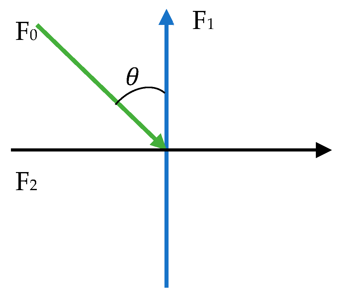
4. Boundary Conditions

Let us consider that along +ve $x_3$-axis a normal point load $F_1$ per unit length acts at the origin and along +ve $x_1$-axis a tangential load $F_2$ per unit length, acts at the origin and due to concentrated normal force on the half space, the dimensionless conditions are given by

i.

Normal stress

$$t_{33}\left(x_1,x_3,t\right)=-F_1\delta \left(x_1\right)H\left(t\right)$$

(43)

ii.

Tangential stress

$$t_{31}\left(x_1,x_3,t\right)=-F_2\delta \left(x_1\right)H\left(t\right)$$

(44)

iii.

Vanishing of tangential couple stress

$$m_{32}\left(x_1,x_3,t\right)=0$$

(45)

iv.

Condition of temperature change

$$\frac{\partial \phi }{\partial x_3}\left(x_1,x_3,t\right)=0$$

(46)

where $F_1$ and $F_2$ are the vertical and horizontal magnitude of the forces applied, $\delta \left(x\right)$ specify the concentrated load distribution function along the x-axis, and $H\left(\right)$ is given by

$$H\left(t\right)=\left\{\begin{array}{c}1, t\ge 0,\\ 0 , t<0\end{array}\right.$$

(47)

$$H\left(s\right)=L\left(H\left(t\right)\right)=\frac{1}{s}.$$

(48)

As an application along the positive boundary $x_3$-axis, a normal point load F₁ is applied at the origin and along the positive $x_1$-axis a load F₂ per unit length and are applied at the origin. Assume an inclined load, F₀ per unit length inclined at an angle $\mathsf{\theta }$ with $x_3$-axis is acting on the $x_2$-axis (see Figure 2):

$${\mathrm{F}}_1={ \mathrm{F}}_0{\cos \mathsf{\theta } \mathrm{and} \mathrm{F}}_2={ \mathrm{F}}_0\sin \mathsf{\theta }.$$

(49)

Using (34)–(36) and (42) in Equations (43)–(46) and then applying the transforms (25) and (28) and hence these equations can be written as

$${\displaystyle \sum }_{j=1}^4{M}_j{A}_j=-\frac{F_1}{s},$$

(50)

$${\displaystyle \sum }_{j=1}^4{N}_j{A}_j=-\frac{F_2}{s},$$

(51)

$${\displaystyle \sum }_{j=1}^4{O}_j{A}_j=0,$$

(52)

$${\displaystyle \sum }_{j=1}^4{P}_j{A}_j=0,$$

(53)

$$M_j=\left({\zeta }_{17}+{\delta }_4{\lambda }_j{d}_j+{\zeta }_9{g}_j\right),$$

$$N_j=\left({\delta }_1{\lambda }_j+{\zeta }_{18}{d}_j\right),$$

$$O_j=\left({\zeta }_3{\lambda }_j^2+{\zeta }_5{d}_j\right),$$

$$P_j=\left({\lambda }_j{h}_{j}i\xi \right).$$

Solving (50)–(53), by Cramer’s rule we get $A_1,A_2,A_3,A_4$ as

$$A_1=\frac{-F_1{\mathrm{Q}}_1+F_2{\mathrm{Q}}_5}{\mathsf{\Lambda }\mathrm{s}},$$

(54)

$$A_2=\frac{F_1{\mathrm{Q}}_2-F_2{\mathrm{Q}}_6}{\mathsf{\Lambda }\mathrm{s}},$$

(55)

$$A_3=\frac{-F_1{\mathrm{Q}}_3+F_2{\mathrm{Q}}_7}{\mathsf{\Lambda }\mathrm{s}},$$

(56)

$$A_4=\frac{F_1{\mathrm{Q}}_4-F_2{\mathrm{Q}}_8}{\mathsf{\Lambda }\mathrm{s}},$$

(57)

where

$${\mathrm{Q}}_1=N_2{R}_{1 }-R_2{N}_3+R_3{N}_4,$$

$${\mathrm{Q}}_5=M_2{R}_{1 }-R_2{M}_3+R_3{M}_4,$$

$${\mathrm{Q}}_2=N_1{R}_{1 }-R_4{N}_3+R_5{N}_4,$$

$${\mathrm{Q}}_6=M_1{R}_{1 }-R_4{M}_3+R_5{M}_4$$

$${\mathrm{Q}}_3=N_1{R}_{2 }-R_4{N}_2+R_6{N}_4,$$

$${\mathrm{Q}}_7=M_1{R}_{2 }-R_4{M}_2+R_6{M}_4$$

$${\mathrm{Q}}_4=N_1{R}_{3 }-R_5{N}_2+R_6{N}_3,$$

$${\mathrm{Q}}_8=M_1{R}_{3 }-R_5{M}_2+R_6{M}_3,$$

$$\mathsf{\Lambda }=M_1{Q}_{1 }-Q_2{M}_2+Q_3{M}_3-Q_4{M}_4,$$

$$R_{1 }=O_3{P}_{4 }-O_4{P}_3,$$

$$R_{2 }=O_2{P}_{4 }-O_4{P}_2,$$

$$R_{3 }=O_2{P}_{3 }-O_3{P}_2,$$

$$R_{4 }=O_1{P}_{4 }-O_4{P}_1,$$

$$R_{5 }=O_1{P}_{3 }-O_3{P}_1,$$

$$R_{6 }=O_1{P}_{2 }-O_2{P}_1.$$

The expressions for displacement components, conductive temperature, thermodynamic temperature, the normal, tangential and couple stress in transformed domain are obtained from (39)–(42) and (34)–(36) by placing the values of $A_1,A_2,A_3,A_4$ from (54)–(57) as

$${\widehat{u}}_1=\frac{F_1}{\mathrm{s}\mathsf{\Lambda }}\left[{{\displaystyle \sum }}_{j=1}^4{\mathrm{Q}}_{\mathrm{j}}{e}^{-{\lambda }_i{x}_3}\right]+\frac{F_2}{\mathrm{s}\mathsf{\Lambda }}\left[{{\displaystyle \sum }}_{j=1}^4{\mathrm{Q}}_{j+4}{e}^{-{\lambda }_i{x}_3}\right],$$

(58)

$${\widehat{u}}_3=\frac{F_1}{\mathrm{s}\mathsf{\Lambda }}\left[{{\displaystyle \sum }}_{j=1}^4{d}_j{\mathrm{Q}}_{\mathrm{j}}{e}^{-{\lambda }_i{x}_3}\right]+\frac{F_2}{\mathrm{s}\mathsf{\Lambda }}\left[{{\displaystyle \sum }}_{j=1}^4{d}_j{\mathrm{Q}}_{j+4}{e}^{-{\lambda }_i{x}_3}\right],$$

(59)

$$\widehat{T}=\frac{F_1}{\mathrm{s}\mathsf{\Lambda }}\left[{{\displaystyle \sum }}_{j=1}^4{g}_j{\mathrm{Q}}_{\mathrm{j}}{e}^{-{\lambda }_i{x}_3}\right]+\frac{F_2}{\mathrm{s}\mathsf{\Lambda }}\left[{{\displaystyle \sum }}_{j=1}^4{g}_j{\mathrm{Q}}_{j+4}{e}^{-{\lambda }_i{x}_3}\right],,$$

(60)

$$\widehat{\phi }=\frac{F_1}{\mathrm{s}\mathsf{\Lambda }}\left[{{\displaystyle \sum }}_{j=1}^4{h}_j{\mathrm{Q}}_{\mathrm{j}}{e}^{-{\lambda }_i{x}_3}\right]+\frac{F_2}{\mathrm{s}\mathsf{\Lambda }}\left[{{\displaystyle \sum }}_{j=1}^4{h}_j{\mathrm{Q}}_{j+4}{e}^{-{\lambda }_i{x}_3}\right],$$

(61)

$$\widehat{t_{13}}=\frac{F_1}{\mathrm{s}\mathsf{\Lambda }}\left[{{\displaystyle \sum }}_{j=1}^4{N}_j{\mathrm{Q}}_{\mathrm{j}}{e}^{-{\lambda }_i{x}_3}\right]+\frac{F_2}{\mathrm{s}\mathsf{\Lambda }}\left[{{\displaystyle \sum }}_{j=1}^4{N}_j{\mathrm{Q}}_{j+4}{e}^{-{\lambda }_i{x}_3}\right],$$

(62)

$$\widehat{t_{33}}=\frac{F_1}{\mathrm{s}\mathsf{\Lambda }}\left[{{\displaystyle \sum }}_{j=1}^4{M}_j{\mathrm{Q}}_{\mathrm{j}}{e}^{-{\lambda }_i{x}_3}\right]+\frac{F_2}{\mathrm{s}\mathsf{\Lambda }}\left[{{\displaystyle \sum }}_{j=1}^4{M}_j{\mathrm{Q}}_{j+4}{e}^{-{\lambda }_i{x}_3}\right],$$

(63)

$$\widehat{m_{32}}=\frac{F_1}{\mathrm{s}\mathsf{\Lambda }}\left[{{\displaystyle \sum }}_{j=1}^4{O}_j{\mathrm{Q}}_{\mathrm{j}}{e}^{-{\lambda }_i{x}_3}\right]+\frac{F_2}{\mathrm{s}\mathsf{\Lambda }}\left[{{\displaystyle \sum }}_{j=1}^4{O}_j{\mathrm{Q}}_{j+4}{e}^{-{\lambda }_i{x}_3}\right].$$

(64)

5. Inversion of the Transforms

To get the result of the problem in physical domain, we will have to invert the transforms in Equations (58)–(64) To find the function $\hat{f}\left(\xi ,x_3,s\right)$, we first invert the Fourier transform using

$$\overline{f}\left(x_1,x_3,t\right)=\frac{1}{2\pi }{{\displaystyle \int }}_{-\infty }^{\infty }{e}^{-i\xi x}\widehat{f}\left(\xi ,x_3, s\right)d\xi =\frac{1}{2\pi }{{\displaystyle \int }}_{-\infty }^{\infty }\left|cos\left(\xi x_1\right)f_e-isin\left(\xi x_1\right)f_o\right|d\xi$$

(65)

where f_e and f_o are, respectively, the odd and even parts of $\widehat{f}\left(\xi ,x_3,s\right).$ Following Honig and Hirdes [37], the Laplace transform function $\tilde{f}\left(x_1,x_3,s\right)$ can be inverted to f($x_1$, $x_3$, t) by

$$f\left(x_1,x_3,t\right)=\frac{1}{2\pi i}\underset{e^{-i\infty }}{\overset{e^{+i\infty }}{{\displaystyle \int }}}\overline{f}\left(x_1,x_3,s\right)e^{-st}ds.$$

(66)

The last step is to calculate the integral in Equation (65). The method for evaluating this integral is described in Press et al. [38]. It involves the use of Romberg’s integration with adaptive step size.

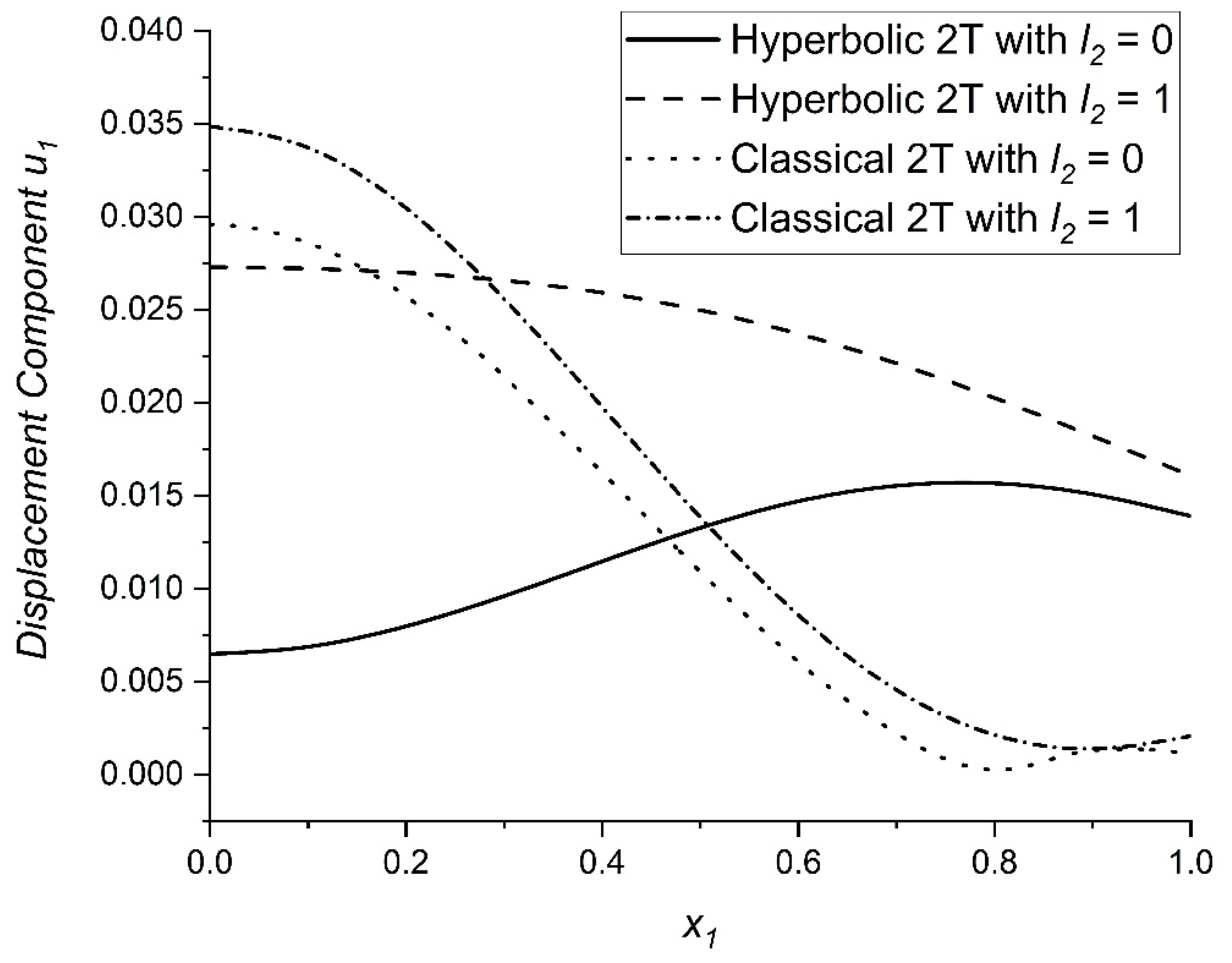
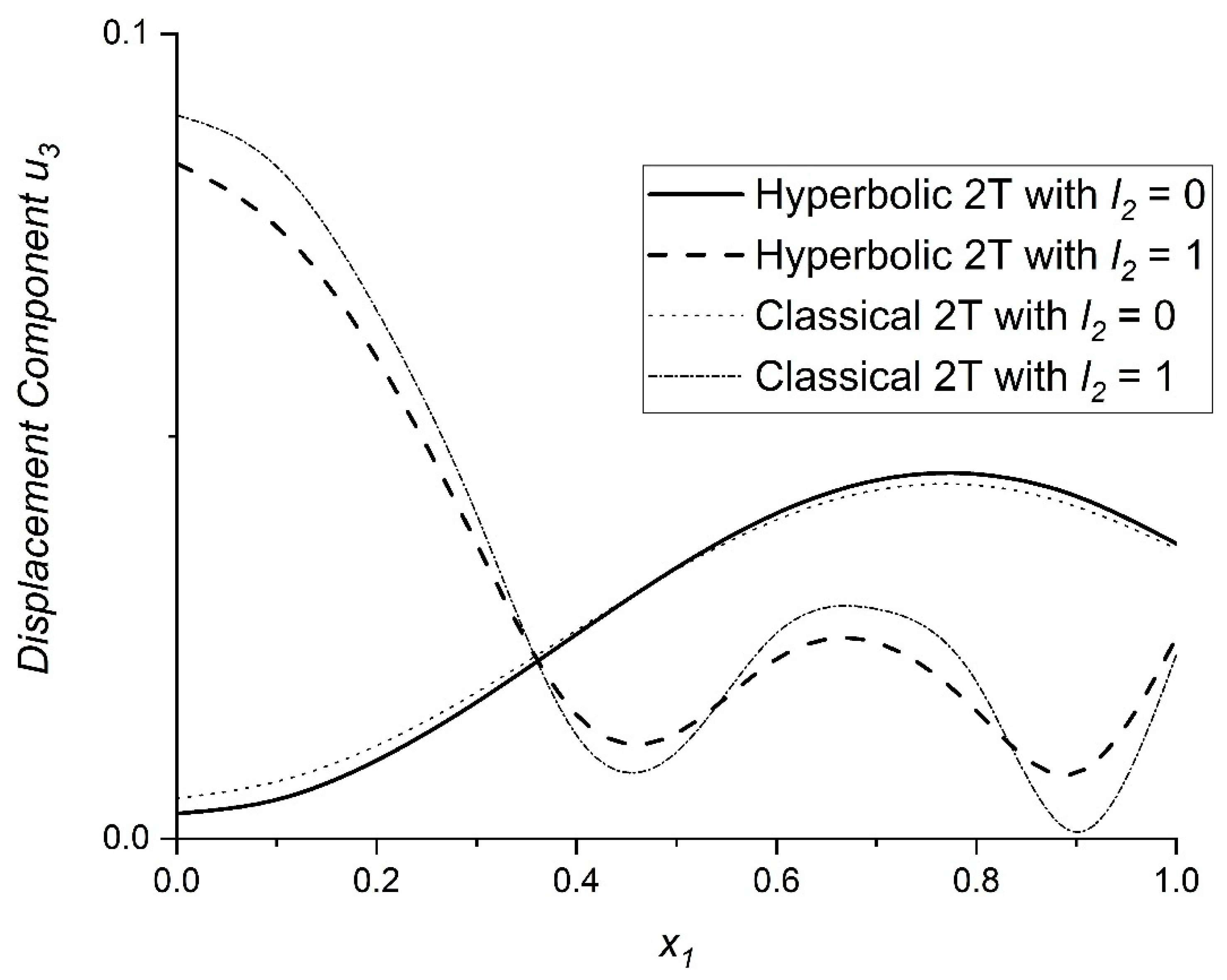
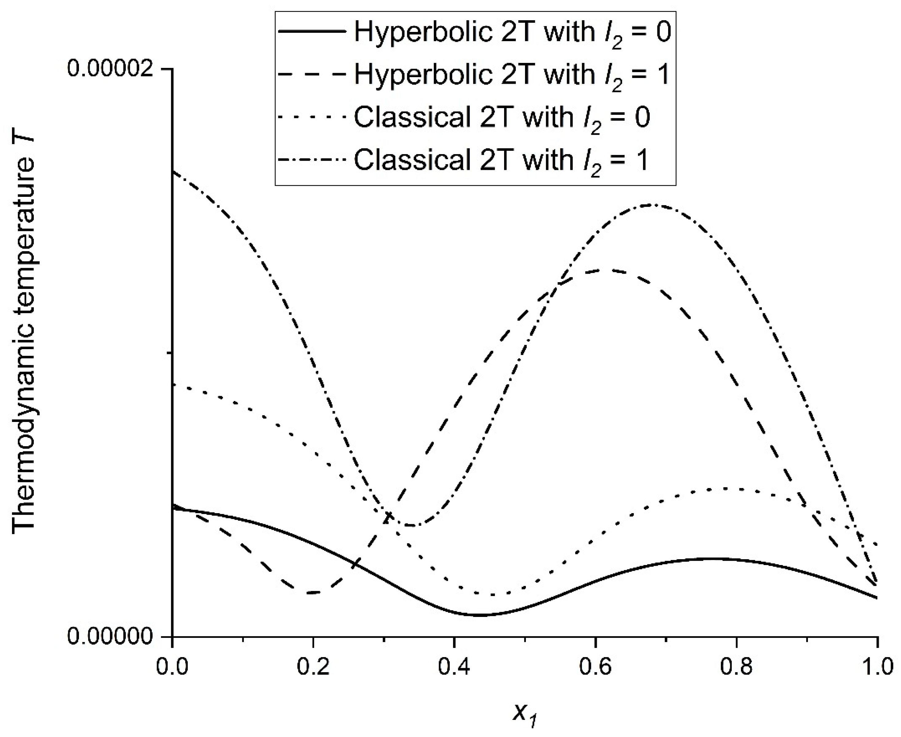
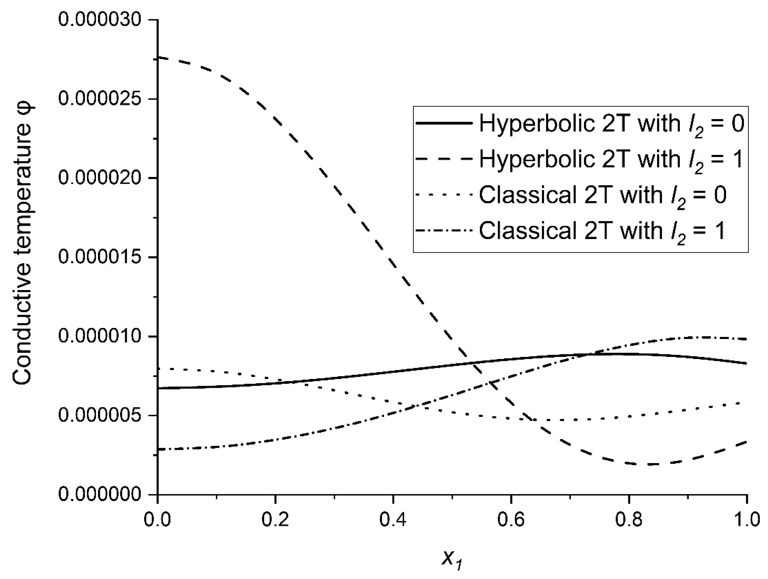
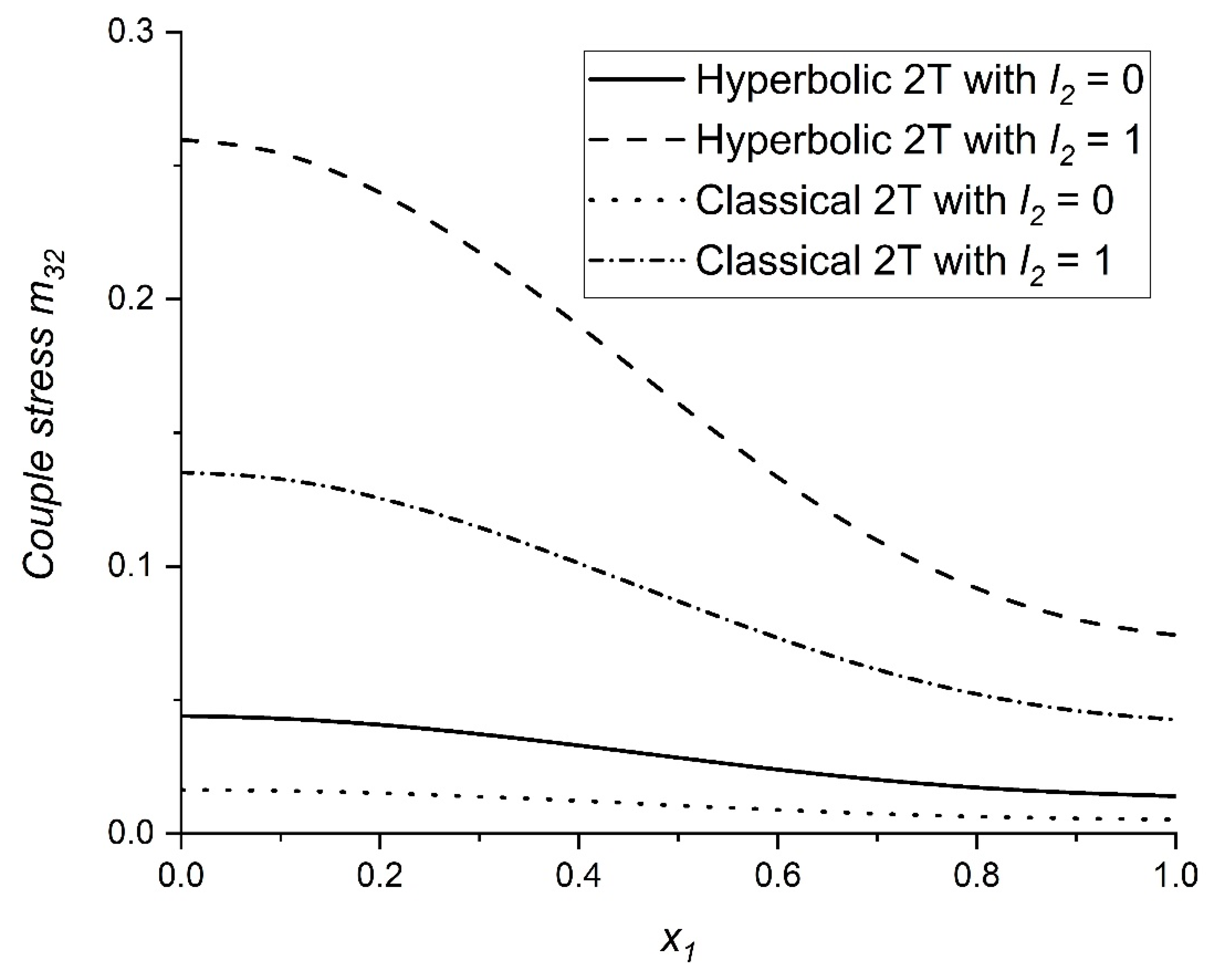
6. Numerical Findings and Interpretation

For numerical computations, computer programming using the software MATLAB has been used and the material constants for a fiber reinforced material are taken from Kumar et al. [39].

$$\lambda =5.65\times {10}^{10} {\mathrm{Nm}}^{-2},{\mu }_T=2.46\times {10}^{10 }{\mathrm{Nm}}^{-2},{\mu }_L=5.66\times {10}^{10} {\mathrm{Nm}}^{-2},$$

$$\beta =220.90\times {10}^{10 }{\mathrm{Nm}}^{-2},C_E=0.787\times {10}^3{\mathrm{Jkg} }^{-1 }{\mathrm{K}}^{-1},K_1=0.0921\times {10}^3{\mathrm{Jm} }^{-1}{ \mathrm{K}}^{-1}{ \mathrm{s}}^{-1},$$

$$K_3=0.0963\times {10}^3{ \mathrm{Jm}}^{-1}{ \mathrm{K}}^{-1}{ \mathrm{s}}^{-1},{\alpha }_1=0.017\times {10}^{-4},{\alpha }_3=0.015\times {10}^{-4},$$

$$\alpha =-1.28\times {10}^{10} {\mathrm{Nm}}^{-2},T_0=293 \mathrm{K},b_1=0.02 {\mathrm{m}}^2,b_3=0.03 {\mathrm{m}}^2,$$

$$G_2=0.2,{\tau }_0=0.1, L=1,l_2=0.843 \mathsf{\mu }\mathrm{m}.$$

The graphs are plotted for t = 0.15. The values of the displacement component $u_1$, displacement component $u_3$, thermodynamic temperature T, normal stress $t_{13}$, conducive temperature $\phi ,$ tangential stress $t_{33}$, and coupled stress $m_{32},$ for nMCST and H2T due to inclined load.

In Figure 3, Figure 4, Figure 5, Figure 6, Figure 7, Figure 8 and Figure 9 the effect of H2T and Classical 2T on the various quantities have been shown.

• The solid line relates to H2T theory with $l_2=0$
• The dashed line relates to H2T theory with $l_2=1$
• The dotted line relates to Classical 2T (C2T) theory with $l_2=0$
• The dot-dashed line relates to Classical 2T (C2T) theory with $l_2=1$

Figure 3 shows the variations of the $u_1$ using nMCST for H2T and C2T with different values of length scale parameter $l_2$. In the initial value of $x_1$, the $u_1$ decreases sharply for H2T with $l_2=1$ and H2T with length scale parameter $l_2=0 \mathrm{and} 1$ and then diminishes to zero for C2T theory. C2T shows a higher variation in the $u_1$. as compared to H2T. Figure 4 illustrates the variations of the $u_3$ using nMCST for H2T and C2T with different values of length scale parameter $l_2$. In the initial value of $x_1,$ and length scale parameter $l_2=1$ the $u_3$ decreases sharply for both H2T and C2T. Moreover In the initial value of $x_1,$ and length scale parameter $l_2=0$ the $u_3$ increases for both H2T and C2T. C2T shows a higher variation in the $u_3$ as compared to H2T. Figure 5 displays the variations of thermodynamic temperature $T$ using nMCST for H2T and C2T with different values of length scale parameter $l_2$. In the initial value of $x_1$, the $T$ decreases sharply and then illustrates a sharp rise in the $T$ for the rest of the value of $x_3$. C2T shows a higher variation in the $T$ as compared to H2T with the length scale parameter $l_2=1$. Figure 6 displays the variations of conductive temperature $\phi$ using nMCST for H2T and C2T with different values of length scale parameter $l_2$. In the initial value of $x_1$, the $\phi$ decreases sharply for H2T with the length scale parameter $l_2=1$ and then shows the oscillatory behavior for the rest of the value of $x_3$. C2T shows a higher variation in the $\phi$ as compared to H2T.

Figure 7 displays the deviations of Normal Stress $t_{13}$ using nMCST for H2T and C2T with different values of length scale parameter $l_2$. In the initial value of $x_1$, the $t_{13}$ increases slowly for H2T and C2T for length scale parameter $l_2=0$ and decreases sharply for H2T and C2T for length scale parameter $l_2=1$. H2T with length scale parameter $l_2=1$ shows a higher variation in the $t_{13}$ as compared to C2T. Figure 8 displays the deviations of tangential Stress $t_{33}$ using nMCST for H2T and C2T with different values of length scale parameter $l_2$. In the initial value of $x_1$, the $t_{33}$ decreases sharply and then shows a slight rise for the rest of the value of $x_3$. H2T shows a higher variation in the $t_{33}$ as compared to C2T. Figure 9 displays the deviations of couple stress $m_{32}$ using nMCST for H2T and C2T with different values of length scale parameter $l_2$. For H2T and C2T, the $m_{32}$ for length scale parameter $l_2=1$ decreases sharply. H2T shows a higher variation in the $m_{32}$ as compared to C2T with length scale parameter.

7. Conclusions

The new modified couple stress theory of thermoelasticity with hyperbolic two-temperature is studied in fibre-reinforced composites. The medium is subjected to a concentrated inclined load. It is a significant problem in solid mechanics to analyze stresses, hyperbolic conductive temperatures, displacement components and couple stresses caused by inclined loads in fibre-reinforced materials. The Lord Shulman heat conduction equation with hyperbolic two-temperature is used to form the model of the problem. Fourier and Laplace integral transforms method are employed to get the results of the mathematical model. Dynamic response of concentrated inclined load is investigated. The effects of hyperbolic and classical two temperature with length scale parameter are represented explicitly on the physical quantities. Classical two-temperature shows a higher variation in the resultant quantities such as hyperbolic conductive temperatures, displacement components as compared to hyperbolic two-temperature. Hyperbolic two-temperature shows less deformation in the displacement components as compared to C2T and shows better results than the C2T theory of thermoelasticity. The length scale parameter shows the major effect on the analyze stresses, hyperbolic conductive temperatures, displacement components and couple stresses with both theories of thermoelasticity. Researchers working in thermomechanical, sensors, resonators, medical science, accelerometers, as well as in future research, should benefit from the results of this research.

References

1. Pipkin, A.C.; Rogers, T.G. Plane Deformations of Incompressible Fiber-Reinforced Materials. J. Appl. Mech. 1971, 38, 634–640. [Google Scholar] [CrossRef]
2. Spencer, A.J.M. Deformations of Fibre-Reinforced Materials. Clarendon Press: Oxford, UK, 1972. [Google Scholar]
3. Pipkin, A.C. Finite Axisymmetric Deformations Of Ideal Fibre-Reinforced Composites. Q. J. Mech. Appl. Math. 1975, 28, 271–284. [Google Scholar] [CrossRef]
4. Testa, R.; Boley, B. Basic thermoelastic problems in fiber-reinforced materials. In Mechanics of Composite Materials; Elsevier: Amsterdam, The Netherlands, 1970; pp. 361–385. [Google Scholar] [CrossRef]
5. Craig, M.S.; Hart, V.G. The Stress Boundary-Value Problem For Finite Plane Deformations Of A Fibre-Reinforced Material. Q. J. Mech. Appl. Math. 1979, 32, 473–498. [Google Scholar] [CrossRef]
6. Rogers, T.G. Finite Deformation and Stress in Ideal Fibre-Reinforced Materials. In Continuum Theory of the Mechanics of Fibre-reinforced Composites; Springer: Vienna, Austria, 1984; pp. 33–71. [Google Scholar] [CrossRef]
7. Bayones, F.S.; Hussien, N.S. Fibre-Reinforced Generalized Thermoelastic Medium Subjected to Gravity Field. J. Mod. Phys. 2015, 6, 1113–1134. [Google Scholar] [CrossRef] [Green Version]
8. Said, S.M. A fiber-reinforced thermoelastic medium with an internal heat source due to hydrostatic initial stress and gravity for the three-phase-lag model. Multidiscip. Model. Mater. Struct. 2017, 13, 83–99. [Google Scholar] [CrossRef]
9. Voigt, W. Theoretische Studien Über Die Elasticitätsverhältnisse der Krystalle; Royal Society of Sciences in Göttingen: Göttingen, Germany, 1887; Available online: https://www.worldcat.org/title/theoretische-studien-uber-die-elasticitatsverhaltnisse-der-krystalle/oclc/634403068 (accessed on 24 June 2021).
10. Cosserat, E.; Cosserat, F. Théorie des Corps déformables. Nature 1909, 81, 67. [Google Scholar] [CrossRef] [Green Version]
11. Mindlin, R.D. Influence of couple-stresses on stress concentrations—Main features of cosserat theory are reviewed by lecturer and some recent solutions of the equations, for cases of stress concentration around small holes in elastic solids, are described. Exp. Mech. 1963, 3, 1–7. [Google Scholar] [CrossRef]
12. Koiter, W.T. Couple-Stresses in the Theory of Elasticity, I & II, Philos. Philos. Trans. R. Soc. Lond. B 1969, 67, 17–44. [Google Scholar]
13. Yang, F.; Chong, A.; Lam, D.; Tong, P. Couple stress based strain gradient theory for elasticity. Int. J. Solids Struct. 2002, 39, 2731–2743. [Google Scholar] [CrossRef]
14. Chen, W.; Li, X. A new modified couple stress theory for anisotropic elasticity and microscale laminated Kirchhoff plate model. Arch. Appl. Mech. 2013, 84, 323–341. [Google Scholar] [CrossRef]
15. Youssef, H. Theory of two-temperature-generalized thermoelasticity. IMA J. Appl. Math. 2006, 71, 383–390. [Google Scholar] [CrossRef]
16. Youssef, H.M. State-Space Approach to Two-Temperature Generalized Thermoelasticity without Energy Dissipation of Medium Subjected to Moving Heat Source. Appl. Math. Mech. 2013, 34, 63–74. [Google Scholar] [CrossRef]
17. Youssef, H.M.; El-Bary, A.A. Theory of hyperbolic two-temperature generalized thermoelasticity. Mater. Phys. Mech. 2018, 40, 158–171. [Google Scholar] [CrossRef]
18. Youssef, H.M. Theory of Generalized Thermoelasticity with Fractional Order Strain. JVC/Journal Vib. Control 2016, 22, 3840–3857. [Google Scholar] [CrossRef]
19. Kaur, I.; Lata, P.; Singh, K. Effect of Hall current in transversely isotropic magneto-thermoelastic rotating medium with fractional-order generalized heat transfer due to ramp-type heat. Indian J. Phys. 2020, 95, 1165–1174. [Google Scholar] [CrossRef]
20. Lata, P.; Kaur, I.; Singh, K. Effect of thermal laser pulse in transversely isotropic Magneto-thermoelastic solid due to Time-Harmonic sources. Coupled Syst. Mech. 2020, 9, 343. [Google Scholar] [CrossRef]
21. Craciun, E.-M.; Baesu, E.; Soós, E. General solution in terms of complex potentials for incremental antiplane states in prestressed and prepolarized piezoelectric crystals: Application to Mode III fracture propagation. IMA J. Appl. Math. 2004, 70, 39–52. [Google Scholar] [CrossRef]
22. Khan, A.A.; Bukhari, S.R.; Marin, M.; Ellahi, R. Effects Of Chemical Reaction On Third-Grade Mhd Fluid Flow Under The Influence Of Heat And Mass Transfer With Variable Reactive Index. Heat Transf. Res. 2019, 50, 1061–1080. [Google Scholar] [CrossRef]
23. Marin, M.; Oechsner, A. The effect of a dipolar structure on the Hölder stability in Green–Naghdi thermoelasticity. Contin. Mech. Thermodyn. 2017, 29, 1365–1374. [Google Scholar] [CrossRef]
24. Singh, A.; Das, S.; Altenbach, H.; Craciun, E.-M. Semi-infinite moving crack in an orthotropic strip sandwiched between two identical half planes. ZAMM J. Appl. Math. Mech. Z. Angew. Math. Mech. 2019, 100, e201900202. [Google Scholar] [CrossRef]
25. Zhang, L.; Bhatti, M.M.; Marin, M.; Mekheimer, K.S. Entropy Analysis on the Blood Flow through Anisotropically Tapered Arteries Filled with Magnetic Zinc-Oxide (ZnO) Nanoparticles. Entropy 2020, 22, 1070. [Google Scholar] [CrossRef] [PubMed]
26. Singh, A.; Das, S.; Craciun, E.-M. Effect of Thermomechanical Loading on an Edge Crack of Finite Length in an Infinite Orthotropic Strip. Mech. Compos. Mater. 2019, 55, 285–296. [Google Scholar] [CrossRef]
27. Marin, M.; Vlase, S.; Paun, M. Considerations on double porosity structure for micropolar bodies. AIP Adv. 2015, 5, 037113. [Google Scholar] [CrossRef] [Green Version]
28. Bhatti, M.M.; Ellahi, R.; Zeeshan, A.; Marin, M.; Ijaz, N. Numerical study of heat transfer and Hall current impact on peristaltic propulsion of particle-fluid suspension with compliant wall properties. Mod. Phys. Lett. B 2019, 33. [Google Scholar] [CrossRef]
29. Bhatti, M.M.; Yousif, M.A.; Mishra, S.R.; Shahid, A. Simultaneous influence of thermo-diffusion and diffusion-thermo on non-Newtonian hyperbolic tangent magnetised nanofluid with Hall current through a nonlinear stretching surface. Pramana 2019, 93, 88. [Google Scholar] [CrossRef]
30. Zhang, L.; Bhatti, M.M.; Michaelides, E.E. Thermally developed coupled stress particle–fluid motion with mass transfer and peristalsis. J. Therm. Anal. Calorim. 2020, 143, 2515–2524. [Google Scholar] [CrossRef]
31. Golewski, G.L. Validation of the favorable quantity of fly ash in concrete and analysis of crack propagation and its length—Using the crack tip tracking (CTT) method—In the fracture toughness examinations under Mode II, through digital image correlation. Constr. Build. Mater. 2021, 296, 122362. [Google Scholar] [CrossRef]
32. Golewski, G.L. Evaluation of fracture processes under shear with the use of DIC technique in fly ash concrete and accurate measurement of crack path lengths with the use of a new crack tip tracking method. Measurement 2021, 181, 109632. [Google Scholar] [CrossRef]
33. Golewski, G.L. The Beneficial Effect of the Addition of Fly Ash on Reduction of the Size of Microcracks in the ITZ of Concrete Composites under Dynamic Loading. Energies 2021, 14, 668. [Google Scholar] [CrossRef]
34. Kaur, I.; Singh, K.; Ghita, G.M.D. New analytical method for dynamic response of thermoelastic damping in simply supported generalized piezothermoelastic nanobeam. ZAMM J. Appl. Math. Mech. Z. Angew. Math. Mech. 2021, 101, e202100108. [Google Scholar] [CrossRef]
35. Kaur, I.; Lata, P.; Singh, K. Study of transversely isotropic nonlocal thermoelastic thin nano-beam resonators with multi-dual-phase-lag theory. Arch. Appl. Mech. 2020, 91, 317–341. [Google Scholar] [CrossRef]
36. Kumar, R.; Garg, S.K.; Ahuja, S. Wave Propagation in Fibre-Reinforced Transversely Isotropic Thermoelastic Media with Initial Stress at the Boundary Surface. J. Solid Mech. 2015, 7, 223–238. [Google Scholar]
37. Honig, G.; Hirdes, U. A method for the numerical inversion of Laplace transforms. J. Comput. Appl. Math. 1984, 10, 113–132. [Google Scholar] [CrossRef] [Green Version]
38. William H. Press; Teukolsky, S.A.; Flannery, B.P. Numerical recipes in Fortran; Cambridge University Press: Cambridge, UK, 1980. [Google Scholar]
39. Kumar, R.; Ahuja, S.; Garg, S.K. Effect of Initial Stress on the Propagation Characteristics of Waves in Fiber-Reinforced Transversely Isotropic Thermoelastic Material under an Inviscid Liquid Layer. J. Thermodyn. 2014, 2014, 34276. [Google Scholar] [CrossRef]
Figure 1. Fiber-reinforced thermoelastic medium.
Mathematics 11 00432 g001
Figure 2. Inclined load over a fiber-reinforced thermoelastic solid.
Mathematics 11 00432 g002
Figure 3. Variations in dimensionless displacement component u 1 .
Mathematics 11 00432 g003
Figure 4. Variations in dimensionless displacement component u 3 .
Mathematics 11 00432 g004
Figure 5. Variations in dimensionless thermodynamic temperature T .
Mathematics 11 00432 g005
Figure 6. Variations in dimensionless conductive temperature φ .
Mathematics 11 00432 g006
Figure 7. Variations in dimensionless Normal Stress t 13 .
Mathematics 11 00432 g007
Figure 8. Variations in dimensionless tangential stress t 33 .
Mathematics 11 00432 g008
Figure 9. Variations in dimensionless couple stress m 32 .
Mathematics 11 00432 g009
Disclaimer/Publisher’s Note: The statements, opinions and data contained in all publications are solely those of the individual author(s) and contributor(s) and not of MDPI and/or the editor(s). MDPI and/or the editor(s) disclaim responsibility for any injury to people or property resulting from any ideas, methods, instructions or products referred to in the content.