Peristalsis of Nanofluids via an Inclined Asymmetric Channel with Hall Effects and Entropy Generation Analysis

Abstract

This study deals with the entropy investigation of the peristalsis of a water–copper nanofluid through an asymmetric inclined channel. The asymmetric channel is anticipated to be filled with a uniform permeable medium, with a constant magnetic field impinging on the wall of the channel. The physical effects, such as Hall current, mixed convection, Ohmic heating, and heat generation/annihilation, are also considered. Mathematical modeling from the given physical description is formulated while employing the “long wavelength, low Reynolds number” approximations. Analytical and numerical procedures allow for the determination of flow behavior in the resulting system, the results of which are presented in the form of tables and graphs, in order to facilitate the physical analysis. The results indicate that the growth of nanoparticle volume fraction corresponds to a reduction in temperature, entropy generation, velocity, and pressure gradient. The enhanced Hall and Brinkman parameters reduce the entropy generation and temperature for such flows, whereas the enhanced permeability parameter reduces the velocity and pressure gradient considerably. Furthermore, a comparison of the heat transfer rates for the two results, for different physical parameters, indicates that these results agree well. The significance of the underlying study lies in the fact that it analyzes the peristalsis of a non-Newtonian nanofluid, where the rheological characteristics of the fluid are predicted using the Carreau-Yasuda model and by considering the various physical effects.

1. Introduction

Peristalsis comprises the contraction and relaxation of muscles of tube-like organs, which facilitates the passage of fluid through such tubes. Such a mechanism is associated with many functional units of the human body, e.g., in the esophagus, wave motions facilitate the movement of food to the stomach, where it is churned into a thick semi-fluid called chyme. Peristalsis continues in the intestines, where the nutrients are absorbed through porous walls. Latham [1] was among the first researchers to analyze peristaltic flow. Later, Shapiro et al. [2] used the approach of “long wavelength, low Reynolds number” to examine peristaltic flows. Lew et al. [3] studied the peristalsis of an incompressible Newtonian fluid passing through the intestine. Since then, numerous studies have been performed to inspect various features of peristalsis [4,5,6,7,8].

Nanofluids are a suspension of nanometer-sized metallic particles in a base fluid, such as water. The notion of nanofluids was proposed by Choi [9,10] in an attempt to enhance the thermal characteristics of ordinary fluids. The improved thermal conductivities of nanofluids compared with other heat transfer fluids are useful in drug delivery, diagnosis and treatment of tumors, industrial/domestic colling, automobile industry, IT industry, and in several other areas of engineering [11,12,13]. The impacts of flexible walls and the effects of the slip parameter on the peristalsis of nanofluids were explored in [14], by Hayat et al., by considering the effects of Joule heating. Ebaid [15] studied the peristaltic movement of Newtonian fluids and explained the effects which occur due to a wall slip condition. Abbasi et al. [16] studied peristalsis while assuming Ohmic heating and Hall effects with nanofluids.

Entropy generation occurs in all real heat transfer processes. A. Bejan [17,18] showed that the entropy generation in a channel is caused by viscous dissipation and heat addition. A. Hijleh et al. [19] examined the entropy generated by natural convection using a numerical analysis of a horizontal cylinder. In a peristaltic flow, Shit and Ranjit [20] investigated the entropy generation under the action of a strong magnetic field. Al-Hadhrami et al. [21] designed a model and investigated viscous dissipation through a porous medium. Hayat et al. [22] analyzed peristalsis in an inclined channel. For analytical purposes, they considered the transport of a Cu-H₂O nanofluid. Ramesh [23] analyzed a non-Newtonian couple stress fluid passing through peristaltic walls by assuming that there is inclined magnetic field, that the medium is porous, and that the asymmetric channel is also inclined. In addition, heat and flow fluid analyses in a wavy microchannel, which is a double-layered sinusoidal heat sink and double-layer microchannel heat sink with sinusoidal cavities and rectangular ribs, have been made in [24,25,26]. A detailed experimental study of thermal conductivity in the case of a hybrid nanofluid was investigated by Boroomandpour et al. [27]. The thermal analysis for a 3-D hollow sphere and circular tube under prescribed non-uniform wall heat flux, and the magneto-hyperbolic-tangent effects for various geometrical settings, have been studied in [28,29,30].

The peristaltic mechanism is considered to be one of the most common fluid transport mechanisms in the human body, via which different fluids are transported from one place to another over short distances. The underlying geometry of peristaltic flow, along with other effects on flow configuration, are only studied because the existing literature lacks investigations of fluid flow in the presence of various physical effects simultaneously. This flow setting is adopted to determine the heat transfer rate from the fluid to the wall of the channel and vice versa, subject to varying physical parameters of interest. Hence, the aim is to analyze the peristalsis of a non-Newtonian nanofluid, where the rheological characteristics of the fluid are predicted using the Carreau-Yasuda model and by considering factors such as the viscous dissipation effect, magnetic field, Ohmic heating, Hall current, mixed convection, and porous medium. Thus, the aims of this study are to focus on the comprehensive analysis of various physical parameters of interest, thereby considering the generation of entropy for the peristalsis of nanofluid through an asymmetric inclined channel. One aim in particular is to study the nanofluid model with heat mass transfer analysis by carrying out the detailed analysis of the physical effects. The governing mathematical model is formulated in Section 2. The non-dimensionalization and unification processes for various physical parameters are carried out in Section 3. Analytical solutions of the resulting nonlinear system are obtained by applying the homotopic perturbation method (HPM) in Section 4. The physical interpretation of the results, along with their validation, is provided in a set of figures and tables presented in Section 5. It is worth noting that such analytical results are validated via the numerical solver NDSolve in Mathematica. The overall investigation has been concluded with some future recommendations in Section 6.

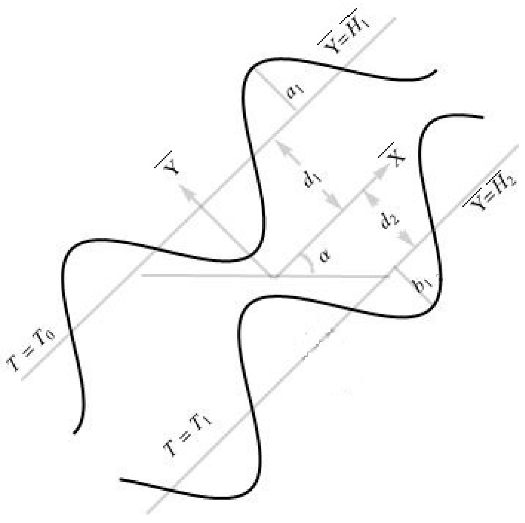
2. Governing Equations

Consider a nanofluid which flows via a two-dimensional asymmetric channel, with thickness (d1 + d2) and inclination at α radians to the horizontal. The nanofluid is composed of copper nanoparticles suspended in water. Flow is produced by periodic waves traveling with uniform speed c on the channel walls/boundaries. Coordinates axes are chosen in a manner such that the channel length ¯Y-axis is normal to it. The geometry of the problem is depicted via Figure 1.

The mathematical expression for peristaltic walls is:

$$\left.\begin{array}{c}\overline{H_1}(\overline{X},\overline{t})=d_1+a_1\hspace{0.17em}\cos (\frac{2\pi }{\lambda }(\overline{X}-c\overline{t})),\\ \overline{H_2}(\overline{X},\overline{t})=-d_2-b_1\hspace{0.17em}\cos (\frac{2\pi }{\lambda }(\overline{X}-c\overline{t})+\gamma ).\end{array}\right\}$$

(1)

Here $\overline{H_1}(\overline{X},\overline{t})$ and $\overline{H_2}(\overline{X},\overline{t})$ denote walls which lies in $\overline{Y}>0$ and $\overline{Y}<0$ regions, respectively, whereas $a_1$ and $b_1$ denote the amplitude of two waves. The difference between their phases is shown by $\gamma .$

Two-dimensional flow is considered, and the channel is considered to be filled with a uniform porous medium with permeability $k_1.$ A magnetic field of strength $B_0$ is incident on the channel in the transverse direction. Hall effects and mixed convection are also considered. The walls $\overline{H_1}(\overline{X},\overline{t})$ and $\overline{H_2}(\overline{X},\overline{t})$ are kept at a fixed temperatures $T_0$ and $T_1$, respectively, with $T_1>T_0.$

The governing equations for such fluid flow models with specific characteristics and effects are considered in [15,16,17]. For a velocity field of the form $\overrightarrow{W}=[\overline{U}\left(\overline{X},\overline{Y},\overline{t}\right),\overline{V}\left(\overline{X},\overline{Y},\overline{t}\right),0]$ (bars denoting the dimensional quantities) considered herein, the governing equations of motion are given as:

$$\frac{\partial \overline{U}}{\partial \overline{X}}+\frac{\partial \overline{V}}{\partial \overline{Y}}=0,$$

(2)

$$\begin{array}{c}{\rho }_{eff}\left(\frac{\partial }{\partial \overline{t}}+\overline{U}\frac{\partial }{\partial \overline{X}}+\overline{V}\frac{\partial }{\partial \overline{Y}}\right)\overline{U}=-\frac{\partial \overline{P}}{\partial \overline{X}}+{\mu }_{eff}\left(\frac{{\partial }^2}{\partial {\overline{X}}^2}+\frac{{\partial }^2}{\partial {\overline{Y}}^2}\right)\overline{U}-\frac{{\mu }_{eff}\overline{U}}{k_1}\\ +g{\left(\rho \beta \right)}_{eff}\left(\overline{T}-T_m\right)\mathit{sin}\hspace{0.17em}\alpha +{\rho }_{eff}g\mathit{sin}\hspace{0.17em}\alpha +\frac{{\sigma }_f{A}_0{B_0}^2}{1+{\left(A_{0}m\right)}^2}\left(-\overline{U}+A_{0}m\overline{V}\right),\end{array}$$

(3)

$$\begin{array}{cc}\hfill {\rho }_{eff}(\frac{\partial }{\partial \overline{t}}+\overline{U}\frac{\partial }{\partial \overline{X}}& +\overline{V}\frac{\partial }{\partial \overline{Y}})\overline{V}\hfill \\ & =-\frac{\partial \overline{P}}{\partial \overline{Y}}+{\mu }_{eff}\left(\frac{{\partial }^2}{\partial {\overline{X}}^2}+\frac{{\partial }^2}{\partial {\overline{Y}}^2}\right)\overline{V}-\frac{{\mu }_{eff}\overline{V}}{k_1}+g{\left(\rho \beta \right)}_{eff}\left(\overline{T}-T_m\right)\mathit{cos}\hspace{0.17em}\alpha \hfill \\ & +{\rho }_{eff}g\mathit{cos}\hspace{0.17em}\alpha -\frac{{\sigma }_f{A}_0{B_0}^2}{1+{\left(A_{0}m\right)}^2}\left(\overline{V}+A_{0}m\overline{U}\right),\hfill \end{array}$$

(4)

$$\begin{array}{c}{\left(\rho Cp\right)}_{eff}\left(\frac{\partial }{\partial \overline{t}}+\overline{U}\frac{\partial }{\partial \overline{X}}+\overline{V}\frac{\partial }{\partial \overline{Y}}\right)\overline{T}=K_{eff}\left(\frac{{\partial }^2}{\partial {\overline{X}}^2}+\frac{{\partial }^2}{\partial {\overline{Y}}^2}\right)\overline{T}+\frac{{\mu }_{eff}\left({\overline{U}}^2+{\overline{V}}^2\right)}{k_1}\\ +{\mu }_{eff}\left[2{\left(\frac{\partial \overline{U}}{\partial \overline{X}}\right)}^2+2{\left(\frac{\partial \overline{V}}{\partial \overline{Y}}\right)}^2+{\left(\frac{\partial \overline{U}}{\partial \overline{Y}}+\frac{\partial \overline{V}}{\partial \overline{X}}\right)}^2\right]\Phi +\frac{{\sigma }_f{A}_0{B_0}^2}{1+{\left(A_{0}m\right)}^2}\left({\overline{V}}^2+{\overline{U}}^2\right).\end{array}$$

(5)

In these equations, $g,\overline{P}\left(\overline{X},\overline{Y},\overline{t}\right),T_m=\frac{T_0+T_1}{2},k_1,$ and $\Phi$ denote acceleration due to gravity, pressure, mean temperature, permeability of porous/permeable medium, and heat generation/absorption parameter, respectively. The Hall parameter $(m)$ and effective electric conductivity $A_0$ are given as [16]:

$$m=\frac{{\sigma }_{eff}{B}_0}{e{n}_e},A_0=\frac{{\sigma }_{eff}}{{\sigma }_f}=\frac{3\left(\frac{{\sigma }_p}{{\sigma }_f}-1\right)\varphi }{\left(\frac{{\sigma }_p}{{\sigma }_f}+2\right)-\left(\frac{{\sigma }_p}{{\sigma }_f}-1\right)\varphi }+1.$$

(6)

Here $e,n_e, \mathrm{a}\mathrm{n}\mathrm{d}, \sigma$ are charge of electron, number density of free electrons, and electric conductivity. For the flow model having two phases, the values of specific heat $(C{p)}_{eff},$ thermal expansion $(\rho \beta {)}_{eff},$ effective density ${\rho }_{eff}$, thermal conductivity $K_{eff},$ and effective viscosity ${\mu }_{eff}$ of nanofluids [16] are as follows:

$$\begin{array}{cc}\hfill (\rho Cp{)}_{eff}=& (\rho Cp{)}_p\varphi -(\varphi -1)(\rho Cp{)}_f,(\rho \beta {)}_{eff}=(\rho \beta {)}_p\varphi -(\varphi -1)(\rho \beta {)}_f,\hfill \\ & {\rho }_{eff}={\rho }_p\varphi -(\varphi -1){\rho }_f,\frac{K_{eff}}{K_f}=\left(\frac{K_p+2\varphi (K_p-K_f)+2K_f}{K_p-\varphi (K_p-K_f)+2K_f}\right),{\mu }_{eff}=\frac{{\mu }_f}{(1-\varphi {)}^{2.5}}.\hfill \end{array}$$

(7)

Here f and p in the subscripts are used to denote the fluid and nanoparticles’ phase, respectively.

3. Non-Dimensionalization Process

In order to determine the flow behaviours using analytical and numerical procedures, the problem is here non-dimensionlized in the laboratory and wave frames. If $\overline{U}$ and $\overline{V}$ define velocity components in $\overline{X}$ and $\overline{Y}$ of the laboratory frame, and $\overline{u}$ and $\overline{v}$ denote velocity components within $\overline{x}$ and $\overline{y}$ of the wave frame, then the transformations between both frame of references are:

$$\overline{x}=\overline{X}-c\overline{t},\overline{y}=\overline{Y},\overline{u}=\overline{U}-c,\overline{v}=\overline{V},\overline{p}\left(\overline{x},\overline{y}\right)=\overline{P}\left(\overline{X},\overline{Y},\overline{t}\right).$$

(8)

In order to express Equations (2)–(5) in non-dimensional form, the following parameters are introduced:

$$\begin{array}{c}u=\frac{\overline{u}}{c},x=\frac{\overline{x}}{\lambda },v=\frac{\overline{v}}{c\delta },\delta =\frac{d_1}{\lambda },y=\frac{\overline{y}}{d_1},a=\frac{a_1}{d_1},b=\frac{b_1}{d_1},d=\frac{d_2}{d_1},h_1=\frac{{\overline{H}}_1}{d_1},p=\frac{{d_1}^2\overline{p}}{c\lambda {\mu }_f},\\ h_2=\frac{{\overline{H}}_2}{d_2},\mathit{Re}\hspace{0.17em}=\frac{{\rho }_{f}c{d}_1}{{\mu }_f},k=\frac{k_1}{{d_1}^2},Gr=\frac{{\rho }_f{\beta }_{f}g{d_1}^2(T_1-T_0)}{{\mu }_{f}c},\theta =\frac{T-T_m}{T_1-T_0},\\ Er=\frac{c^2}{C_f(T_1-T_0)},\mathit{Pr}\hspace{0.17em}=\frac{{\mu }_f{Cp}_f}{K_f},Br=\mathit{Pr}\hspace{0.17em}Er,\in =\frac{d^2\Phi }{(T_1-T_0)K_f},\\ M=\sqrt{\frac{{\sigma }_f}{{\mu }_f}}{B}_0{d}_1,Fr=\frac{c^2}{g{d}_1},u=\frac{\partial \psi }{\partial y},v=-\frac{\partial \psi }{\partial x}.\end{array}$$

(9)

The nomenclature of the quantities used here is provided at the start.

Implementing the small wavelength approximation for Reynolds number and long wavelength, i.e., $\delta \approx 0,$ and dimensionless expressions of Equation (7) in Equations (2)–(5), gives:

$$\frac{\partial p}{\partial x}=A_1\frac{{\partial }^3\psi }{\partial y^3}+A_{2}Gr\theta \mathit{sin}\hspace{0.17em}\alpha -\left[\frac{M^2{A}_0}{1+{\left(A_{0}m\right)}^2}+\frac{A_1}{k}\right]\left[1+\frac{\partial \psi }{\partial y}\right],$$

(10)

$$\frac{\partial p}{\partial y}=0,$$

(11)

$$A_5\frac{{\partial }^2\theta }{\partial y^2}+A_{1}Br{\left(\frac{{\partial }^2\psi }{\partial y^2}\right)}^2+\left[\frac{Br{A}_0{M}^2}{1+{\left(A_{0}m\right)}^2}+\frac{Br{A}_1}{k}\right]{\left(1+\frac{\partial \psi }{\partial y}\right)}^2+\in =0.$$

(12)

Use of the stream function satisfies the continuity equation identically. In the above equations, the $A_s$ are given as:

$$A_1=\frac{1}{(1-\varphi {)}^{2.5}},A_2=1-\varphi +\varphi \frac{(\rho \beta {)}_p}{(\rho \beta {)}_f},A_5=\left(\frac{K_p+2\varphi (K_p-K_f)+2K_f}{K_p-\varphi (K_p-K_f)+2K_f}\right).$$

Cross differentiation of Equations (10) and (11) yields:

$$A_1\frac{{\partial }^4\psi }{\partial y^4}+A_{2}Gr\mathit{sin}\hspace{0.17em}\alpha \frac{\partial \theta }{\partial y}-\left[\frac{M^2{A}_0}{1+{\left(A_{0}m\right)}^2}+\frac{A_1}{k}\right]\left[\frac{{\partial }^2\psi }{\partial y^2}\right]=0.$$

Thermo-physical properties of this system are tabulated in

Table 1. Thermo-physical properties of copper and water [31,32].

Property	Base Fluid (Water)	Copper
$\rho (\mathrm{k}\mathrm{g}·{\mathrm{m}}^{-3})$	997.1	8933
$K (\mathrm{W}·(\mathrm{m}·\mathrm{K}{)}^{-1})$	0.613	401
$Cp (\mathrm{J}·(\mathrm{k}\mathrm{g}·\mathrm{K}{)}^{-1})$	4179	385
$\beta ({\mathrm{K}}^{-1})\times {10}^{-6}$	210	16.65
$\sigma (\mathrm{S}·{\mathrm{m}}^{-1})$	0.05	5.96 × 107

.

Volumetric flow rates in the frames (fixed and moving) are given as:

$$\overline{\eta }={\int }_{{\overline{H}}_2}^{\overline{H_1}}\overline{U}(\overline{X},\overline{Y},\overline{t})d\overline{Y},$$

$$f={\displaystyle \underset{{\overline{H}}_2}{\overset{\overline{H_1}}{\int }}\overline{u}(\overline{x},\overline{y},t)d\overline{y}},$$

and the mean time-averaged flow rate is interpreted as:

$$\overline{Q}=\frac{1}{t_p}{\int }_0^{t_p}\eta dt.$$

Defining dimensionless forms $\eta =\frac{\overline{Q}}{d_{1}c}$ and $F=\frac{f}{d_{1}c}$, the two flow rates are related by:

$$\eta =F+1+d.$$

Furthermore, ‘$F$’ can be computed as:

$$F={\int }_{h_2}^{h_1}\frac{\partial \psi }{\partial y}dy,$$

$$F=\psi (h_1)-\psi (h_2).$$

In the case of velocity and temperature, the non-dimensional no-slip conditions are given by:

$$\psi =\frac{F}{2}, \frac{\partial \psi }{\partial y}=-1,\theta =-\frac{1}{2} at y=h_1\left(x\right),$$

(13a)

$$\psi =-\frac{F}{2}, \frac{\partial \psi }{\partial y}=-1, \theta =\frac{1}{2} at y=h_2\left(x\right).$$

(13b)

Thus, the final system in dimensionless form is given by:

$$A_1\frac{{\partial }^4\psi }{\partial y^4}+A_{2}Gr\mathit{sin}\hspace{0.17em}\alpha \frac{\partial \theta }{\partial y}-\left[\frac{M^2{A}_0}{1+{\left(A_{0}m\right)}^2}+\frac{A_1}{k}\right]\left[\frac{{\partial }^2\psi }{\partial y^2}\right]=0,$$

(14)

and

$$A_5\frac{{\partial }^2\theta }{\partial y^2}+A_{1}Br{\left(\frac{{\partial }^2\psi }{\partial y^2}\right)}^2+\left[\frac{Br{A}_0{M}^2}{1+{\left(A_{0}m\right)}^2}+\frac{Br{A}_1}{k}\right]{\left(1+\frac{\partial \psi }{\partial y}\right)}^2+\in =0.$$

(15)

Subject to non-dimensional conditions at the boundary:

$$\psi =\frac{F}{2},\frac{\partial \psi }{\partial y}=-1,\theta =-\frac{1}{2},aty=h_1\left(x\right),$$

(16a)

$$\psi =-\frac{F}{2},\frac{\partial \psi }{\partial y}=-1,\theta =\frac{1}{2},aty=h_2(x),$$

(16b)

where $h_1(x)=1+a\mathit{cos}\hspace{0.17em}(2\pi x)$ and $h_2(x)=-d-b\mathit{cos}\hspace{0.17em}(2\pi x+\gamma )$ are dimensionless peristaltic profiles.

4. Entropy Generation

The volumetric entropy generation in the dimensional form is given as follows [17,18,19]:

$$\begin{array}{c}{S}_g=\frac{K_{eff}}{{T_0}^2}\left[{\left(\frac{\partial \overline{U}}{\partial \overline{X}}\right)}^2+{\left(\frac{\partial \overline{V}}{\partial \overline{Y}}\right)}^2\right]+\frac{1}{T_0}\left[\frac{{\sigma }_f{A}_0{B_0}^2}{1+{\left(A_{0}m\right)}^2}\left({\overline{V}}^2+{\overline{U}}^2\right)\right]+2\left(\frac{{\mu }_{eff}}{T_0}\right)\\ \left[{\left(\frac{\partial \overline{U}}{\partial \overline{X}}\right)}^2+{\left(\frac{\partial \overline{V}}{\partial \overline{Y}}\right)}^2+\frac{1}{2}{\left(\frac{\partial \overline{U}}{\partial \overline{Y}}+\frac{\partial \overline{V}}{\partial \overline{X}}\right)}^2\right]+\frac{\Phi }{T_0}+\frac{{\mu }_{eff}({\overline{U}}^2+{\overline{V}}^2)}{T_{0}k}.\end{array}$$

(17)

In this equation, entropy generation is caused by heat transport irreversibility, by the magnetic field’s contribution, through heat absorption, by viscous heating, and by the porous medium, respectively.

Entropy generation number $N_S$ is defined as:

$$N_S=A_5{\left(\frac{\partial \theta }{\partial y}\right)}^2+A_{1}Br{\left(\frac{{\partial }^2\psi }{\partial y^2}\right)}^2+\left[\frac{Br{A}_0{M}^2}{1+{\left(A_{0}m\right)}^2}+\frac{Br{A}_1}{k}\right]{\left(1+\frac{\partial \psi }{\partial y}\right)}^2+\epsilon$$

(18)

and Bejan number is given by:

$$Be=\frac{A_5{\left(\frac{\partial \theta }{\partial y}\right)}^2}{A_5{\left(\frac{\partial \theta }{\partial y}\right)}^2+Br{A}_1{\left(\frac{{\partial }^2\psi }{\partial y^2}\right)}^2+\left[\frac{Br{A}_0{M}^2}{1+{\left(A_{0}m\right)}^2}+\frac{Br{A}_1}{k}\right]{\left(1+\frac{\partial \psi }{\partial y}\right)}^2+\epsilon }.$$

(19)

The Bejan number shows the fraction of entropy generated by the irreversibility of heat transportation to the total entropy generation. In the subsequent part of the study, a mathematical procedure to determine the nanofluid flow behaviours is developed.

5. Solution Methodology

Analytical solutions to the governing problem formulated in the previous section are rendered using the perturbation method of the homotopic type. The numerical solutions are determined using a built-in solver in Mathematica, which is further compared with the analytical results. The procedure for the analytical solution is briefly given as:

5.1. Construction of Homotopy

Let

$$H(u,q)=q[A(u)-f(r)]+(1-q)[L(u)-L(u_0)].$$

For the stream function, assume that

$$A(u)-f(r)=A_1\frac{{\partial }^4\psi }{\partial y^4}+A_{2}Gr(\mathit{sin}\hspace{0.17em}\alpha )\frac{\partial \theta }{\partial y}-\left[\frac{M^2{A}_0}{1+{\left(A_{0}m\right)}^2}+\frac{A_1}{k}\right]\left[\frac{{\partial }^2\psi }{\partial y^2}\right],$$

$$L(u)=A_1\frac{{\partial }^4\psi }{\partial y^4},L(u_0)=A_1\frac{{\partial }^4{\psi }_0}{\partial y^4},$$

Using the above equations:

$$\begin{array}{c}H(\psi ,q)=(1-q)\left[A_1\frac{{\partial }^4\psi }{\partial y^4}-A_1\frac{{\partial }^4{\psi }_0}{\partial y^4}\right]\\ +q\left[A_1\frac{{\partial }^4\psi }{\partial y^4}+A_{2}Gr\mathit{sin}\hspace{0.17em}\alpha \frac{\partial \theta }{\partial y}-\left[\frac{M^2{A}_0}{1+{\left(A_{0}m\right)}^2}+\frac{A_1}{k}\right]\left[\frac{{\partial }^2\psi }{\partial y^2}\right]\right]\end{array}$$

For $\theta$ function, let

$$A(u)-f(r)=A_5\frac{{\partial }^2\theta }{\partial y^2}+A_{1}Br{\left(\frac{{\partial }^2\psi }{\partial y^2}\right)}^2+\left[\frac{Br{A}_0{M}^2}{1+{\left(A_{0}m\right)}^2}+\frac{Br{A}_1}{k}\right]{\left(1+\frac{\partial \psi }{\partial y}\right)}^2+\in =0.$$

$$L\left(u\right)=A_5\frac{{\partial }^2\theta }{\partial y^2},L\left(u_0\right)=A_5\frac{{\partial }^2{\theta }_0}{\partial y^2}.$$

Following the similar procedure, we get:

$$\begin{array}{c}H(\theta ,q)=(1-q)\left[A_5\frac{{\partial }^2\theta }{\partial y^2}-A_5\frac{{\partial }^2{\theta }_0}{\partial y^2}\right]\\ +q\left[A_5\frac{{\partial }^2\theta }{\partial y^2}+A_{1}Br{\left(\frac{{\partial }^2\psi }{\partial y^2}\right)}^2+\left[\frac{Br{A}_0{M}^2}{1+{\left(A_{0}m\right)}^2}+\frac{Br{A}_1}{k}\right]{\left(1+\frac{\partial \psi }{\partial y}\right)}^2+\in \right].\end{array}$$

Here, ‘q’ is the embedding parameter and $q\in [0,1].$

The quantities involved above are expanded in the form of a series as:

$$\psi ={\psi }_0+q{\psi }_1+q^2{\psi }_2+q^3{\psi }_3+\cdots$$

$$\theta ={\theta }_0+q{\theta }_1+q^2{\theta }_2+q^3{\theta }_3+\cdots$$

$$F=f_0+q{f}_1+q^2{f}_2+q^3{f}_3+\cdots$$

Then the perturbed system takes the following form:

5.2. Zeroth-Order System

For $\psi :$

$$A_1{{\psi }_0}^{\prime \prime \prime \prime }(y)=0,$$

with boundary conditions

$${\psi }_0(h_1)=\frac{f_0}{2},{{\psi }_0}^{\prime }(h_1)=-1,{\psi }_0(h_2)=\frac{-f_0}{2},{{\psi }_0}^{\prime }(h_2)=-1.$$

For $\theta$:

$$A_5{{\theta }_0}^{\prime \prime }(y)=0,$$

with boundary conditions

$${\theta }_0(h_1)=\frac{-1}{2},{\theta }_0(h_2)=\frac{1}{2}.$$

5.3. First-Order System

For $\psi$:

$$A_1{{\psi }_1}^{\prime \prime \prime \prime }\left(y\right)+A_{2}Gr{{\theta }_0}^{\prime }\left(y\right)\sin \hspace{0.17em}\alpha -\frac{M^2{A}_{0}k+A_1(1+m^2{A}_0^2)({{\psi }_0}^{\prime \prime }(y))}{k(1+m^2{A}_0^2)}=0,$$

with boundary conditions

$${\psi }_1(h_1)=\frac{f_1}{2},{{\psi }_1}^{\prime }(h_1)=0,{\psi }_1(h_2)=\frac{-f_1}{2},{{\psi }_0}^{\prime }(h_2)=0.$$

For $\theta :$

$$A_5{{\theta }_1}^{\prime \prime }(y)+Br{A}_1({{\psi }_0}^{\prime \prime }(y){)}^2+\left[\frac{M^2{A}_{0}Br}{1+m^2{A}_0^2}+\frac{A_{1}Br}{k}\right](1+2{{\psi }_0}^{\prime }(y)+({{\psi }_0}^{\prime }(y){)}^2)+\in =0,$$

with boundary conditions

$${\theta }_1(h_1)=0,{\theta }_1(h_2)=0.$$

5.4. Second-Order System

For $\psi :$

$$A_1{{\psi }_2}^{\prime \prime \prime \prime }\left(y\right)+A_{2}Gr{{\theta }_1}^{\prime }\left(y\right)\sin \hspace{0.17em}\alpha -\frac{M^2{A}_{0}k+A_1(1+m^2{A}_0^2)({{\psi }_1}^{\prime \prime }(y))}{k(1+m^2{A}_0^2)}=0,$$

with boundary conditions

$${\psi }_2(h_1)=\frac{f_2}{2},{{\psi }_2}^{\prime }(h_1)=0,{\psi }_2(h_2)=\frac{-f_2}{2},{{\psi }_2}^{\prime }(h_2)=0.$$

For $\theta :$

$$A_5{{\theta }_2}^{\prime \prime }(y)+2Br{A}_1{{\psi }_0}^{\prime \prime }(y){{\psi }_1}^{\prime \prime }(y)+\left[\frac{2M^2{A}_{0}Br}{1+m^2{A}_0^2}+\frac{2A_{1}Br}{k}\right]({{\psi }_0}^{\prime }(y){{\psi }_1}^{\prime }(y)+{{\psi }_1}^{\prime }(y))=0,$$

with boundary conditions

$${\theta }_2(h_1)=0,{\theta }_2(h_2)=0.$$

The results are retained up to the second order of approximation.

These results are further detailed and compared with the numerical findings in the subsequent analysis.

6. Results and Discussion

This section performs the graphical analysis of the obtained results in the aforementioned study. The impact of flow and geometric parameters (i.e., volume fraction of nanoparticles (ϕ), Hartman number (M), heat absorption or generation parameter (ϵ), Brinkman number (Br), permeability parameter (k), Hall parameter (m) on velocity (u), dimensionless entropy generation (Ns), streamwise pressure gradient (dp/dx), temperature (θ), and Bejan number (Be) are analyzed.

The temperature investigation for variations in different combinations of geometry and flow parameters is provided through Figure 2, Figure 3, Figure 4, Figure 5, Figure 6, Figure 7 and Figure 8. It can be seen, via Figure 2, that the inclusion of copper nanoparticles reduces the temperature of the base fluid because nanoparticles boost the specific heat capacity of the nanofluid and augment the heat transport. Figure 3 shows that increasing the magnetic field increases the fluid’s temperature. Conversely, a reduction in the nanofluid temperature is obtained by assigning higher values to the Hall parameter (see Figure 4). This agrees with the fact that the Hall parameter reduces the effects of the applied magnetic field. Figure 5 shows that there is a decrement in temperature for growing values of permeability parameter. Figure 6 shows that the temperature is greatly affected by the heat absorption/generation parameter. Figure 7 indicates that an increment in Brinkman number enhances the temperature of the nanofluid. At higher values of the Brinkman number, the heat production rate through viscous dissipation rises and this increases the temperature of the Cu-H₂O nanofluid. Figure 8 is plotted to analyze the influence of the Grashof number on the temperature of the nanofluid. It shows that the higher temperature values close to the center of the channel are due to the flow undergoing mixed convection.

Figure 9, Figure 10, Figure 11, Figure 12, Figure 13, Figure 14 and Figure 15 analyze the behavior of the axial velocity (u) through changing values of the nanoparticle volume fraction, Hall parameter, heat generation/absorption parameter, permeability parameter, Brinkman number, Grashof number, and Hartman number. Figure 9 shows that increasing the nanoparticle volume fraction reduces the velocity of the fluid. Increasing the Hartman number decelerates the axial velocity, but the reverse effect is obtained by increasing the Hall parameter (see Figure 10 and Figure 11). Figure 12 shows that the axial velocity of the nanofluid rises by a small amount for growing values of the permeability parameter. Figure 13 shows that, when heat absorption/generation rate is high, a higher nanofluid is obtained. For positive increasing values of the Brinkman number, the axial flow velocity increases a little (see Figure 14). Figure 15 analyzes the effect of the Grashof number on the axial velocity of the nanofluid. It shows that higher values (which are close to center of the channel) of velocity are obtained when the flow has a mixed convection effect.

Figure 16, Figure 17, Figure 18, Figure 19, Figure 20, Figure 21 and Figure 22 were plotted to examine the behavior of the pressure gradient for variations in geometry and flow parameters. These figures show the spatially periodic nature of the streamwise pressure gradient. The spatial pattern of the streamwise pressure gradient repeats over one full wavelength. For growing values of the copper nanoparticle volume fraction, fluid is more viscous. Therefore, in regions of greater channel width, a modest reduction in streamwise pressure gradient is observed, and in the region where channel width is small, a reduction in streamwise pressure gradient is noted (see Figure 16). Figure 17 shows that when the Hartman number rises, the Lorentz force opposes the flow. Hence, a considerable decrement in the streamwise pressure gradient occurs over a vast area, while an increment is observed in the narrower region of the peristaltic walls. Figure 18 shows that the pressure gradient increases over a wide area of peristaltic wall when the Hall parameter is assigned higher values. For rising values of the permeability parameter, fluid motion is faster. This produces a considerable increment in the pressure gradient in wider sections of the peristaltic channel and a small decrement in the occluded sections of the peristaltic channel (see Figure 19). With an increment in the absorption/generation of the heat parameter, the streamwise pressure gradient increases (see Figure 20). Figure 21 shows that the streamwise pressure gradient grows by increasing the Grashof number. This implies that the streamwise pressure gradient is great for mixed convective heat transfer phenomena. The high values of the Grashof number show that viscous forces are less dominant than buoyancy forces. With an increment in Brinkman number, viscous heat production is high and the streamwise pressure gradient increases (see Figure 22).

By assigning positive values to the nanoparticle volume fraction, permeability parameter, Hall parameter, heat generation/absorption parameter, Brinkman number, Grashof number, and Hartman number, a variation in entropy generation is observed (see Figure 23, Figure 24, Figure 25, Figure 26, Figure 27, Figure 28 and Figure 29). Figure 23 shows that a reduction in entropy generation occurs for growing rates of nanoparticle volume fraction. From Figure 24, it can be seen that when Hartman number increases, entropy generation increases. This implies that an increase in the strength of the applied magnetic field results in an increase in temperature; as a result, entropy increases. When Hall effects are raised, entropy generation declines (see Figure 25). This agrees with the fact that the Hall parameter reduces the resistive effect of the magnetic field. Figure 26 illustrates that, with the growth of the absorption/generation of the heat parameter, entropy generation increases. Figure 27 shows that for increasing the value of the permeability parameter, the motion of the fluid through the channel is faster. Entropy generation decreases by a small amount along the lower wall of the channel as the Grashof number rises (see Figure 28). Figure 29 illustrates that with the growth of Brinkman number, entropy generation increases.

Figure 30, Figure 31, Figure 32, Figure 33, Figure 34, Figure 35 and Figure 36 are shown to interpret the effects of nanoparticle volume fraction, permeability parameter, Hall parameter, heat generation/absorption parameter, Brinkman number, Grashof number, and Hartman number on Bejan number (Be). When the number of copper nanoparticles increases, a decrement in Bejan number is observed (see Figure 30). The Bejan number shows the fraction of entropy generated by the irreversibility of heat transportation to the total entropy generation. By adding copper nanoparticles, the fluid becomes more viscous. For increasing values of the Hartman number, there is an increase in the strength of the applied magnetic field. An increment in Bejan number is predicted at larger Hartman number values (see Figure 31). Figure 32 shows that rising values of the Hall parameter reduces the resistive effect of the magnetic field, which causes a reduction in the Bejan number by a very small amount. Analysis of Figure 33 indicates that for an increasing rate of the heat generation/absorption, the Bejan number increases by a significant amount around the channel walls, and a decreasing trend is noticed in the center of the channel. Figure 34 shows that for increasing the rate of permeability parameter, the Bejan number decreases. Increments in the Grashof number show a very small increment in the Bejan number along the wall (see Figure 35). It can be seen from Figure 36 that an increment in the Bejan number occurs when the Brinkman number increases.

After the detailed analyses presented above, it is worth mentioning that various physical aspects associated with the parameters of interest can further be illustrated with the help of Equations (6) and (9). It was stated that these equations describe the direct and indirect relationships among various parameters; thus, the effect of one physical parameter with respect to another parameter can be illustrated further through these relations. It should be noted that these relations are established as a consequence of certain physical laws. Therefore, an explanation of flow behaviour with respect to different flow parameters is in accordance with the physical aspects of fluid flow.

The validation of the results obtained above is provided in the subsequent explanation.

Validation of the Results

Here, a comparison of numerical results is made with that of analytical results in a quantitative manner for various physical parameters. The comparison is made while measuring the heat transfer rate at the upper wall of the channel by varying the nanoparticle volume fraction, Hall parameter, and Brinkman number. To this end,

Table 2. Heat transfer rate at the upper boundary by varying nanoparticle volume fraction, where $\gamma =\frac{\pi }{4},\alpha =\frac{\pi }{4},\eta =0.8,a=0.6,d=0.7,b=0.5,x=0,Br=0.2,k=2,$ $Gr=2,m=1,\in =2,M=1$.

$\mathit{\varphi }$	$\mathbf{Numerical}\mathbf{Values}\mathbf{of}-\frac{{\mathit{k}}_{\mathit{e}\mathit{f}\mathit{f}}}{{\mathit{k}}_{\mathit{k}}}{\mathit{\theta }}^{\prime }({\mathit{h}}_1)$	$\mathbf{Homotopy}\mathbf{Perturbation}\mathbf{Values}\mathbf{of}-\frac{{\mathit{k}}_{\mathit{e}\mathit{f}\mathit{f}}}{{\mathit{k}}_{\mathit{k}}}{\mathit{\theta }}^{\prime }({\mathit{h}}_1)$	Difference %
0.0	3.3471	3.34155	0.55
0.03	3.3999058	3.39625	0.36
0.06	3.4574883	3.45552	0.19
0.09	3.5203507	3.51908	0.12

,

Table 3. Heat transfer rate at the upper boundary by changing Hall parameter, where $\gamma =\frac{\pi }{4},\alpha =\frac{\pi }{4},\eta =0.8,a=0.6,d=0.7,b=0.5,x=0,Br=0.2,k=2,Gr=2,\varphi =0.05,$ $\in =2,M=1$.

m	$\mathbf{Numerical}\mathbf{Values}\mathbf{of}-\frac{{\mathit{k}}_{\mathit{e}\mathit{f}\mathit{f}}}{{\mathit{k}}_{\mathit{f}}}{\mathit{\theta }}^{\prime }({\mathit{h}}_1)$	$\mathbf{Homotopy}\mathbf{Perturbation}\mathbf{Values}\mathbf{of}-\frac{{\mathit{k}}_{\mathit{e}\mathit{f}\mathit{f}}}{{\mathit{k}}_{\mathit{f}}}{\mathit{\theta }}^{\prime }({\mathit{h}}_1)$	Difference %
0.5	3.48729	3.487743	0.045
1.0	3.43773	3.435047	0.4
1.5	3.41023	3.405980	0.42
2.0	3.39607	3.391042	0.52

and

Table 4. Heat transfer rate at the upper boundary by changing Brinkman number, where $\gamma =\frac{\pi }{4},\alpha =\frac{\pi }{4},\eta =0.8,a=0.6,d=0.7,b=0.5,x=0,k=2,m=1,Gr=2,M=1,\in =2,\varphi =0.05$.

Br	$\mathbf{Numerical}\mathbf{Values}\mathbf{of}-\frac{{\mathit{k}}_{\mathit{e}\mathit{f}\mathit{f}}}{{\mathit{k}}_{\mathit{k}}}{\mathit{\theta }}^{\prime }({\mathit{h}}_1)$	$\mathbf{Homotopy}\mathbf{Perturbation}\mathbf{Values}\mathbf{of}-\frac{{\mathit{k}}_{\mathit{e}\mathit{f}\mathit{f}}}{{\mathit{k}}_{\mathit{k}}}{\mathit{\theta }}^{\prime }({\mathit{h}}_1)$	Difference %
0.0	3.089619	3.089619	0.00000
0.2	3.437732	3.435047	0.26
0.4	3.789015	3.781528	0.74
0.6	4.144163	4.129062	1.5

are provided to yield a comparison of the results obtained analytically and numerically. It can be seen that the numerical estimation of heat transfer at the wall shows good comparison between the two results. Furthermore, these tables show the behavior of heat transfer rates for deviations in the volume fraction of nanoparticles, Hall parameter, and Brinkman number. These tables complement the observations of the graphs.

7. Conclusions

The peristalsis of a nanofluid (composed of copper nanoparticles suspended in water) passing through an asymmetric and inclined channel with mixed convection, porous medium, Ohmic heating, Hall current, and heat absorption/generation effects has been examined. The aim of the study was to determine how the consideration of different physical parameters affects the heat transfer rate through the channel. In view of the detailed analysis conducted, it has been concluded that:

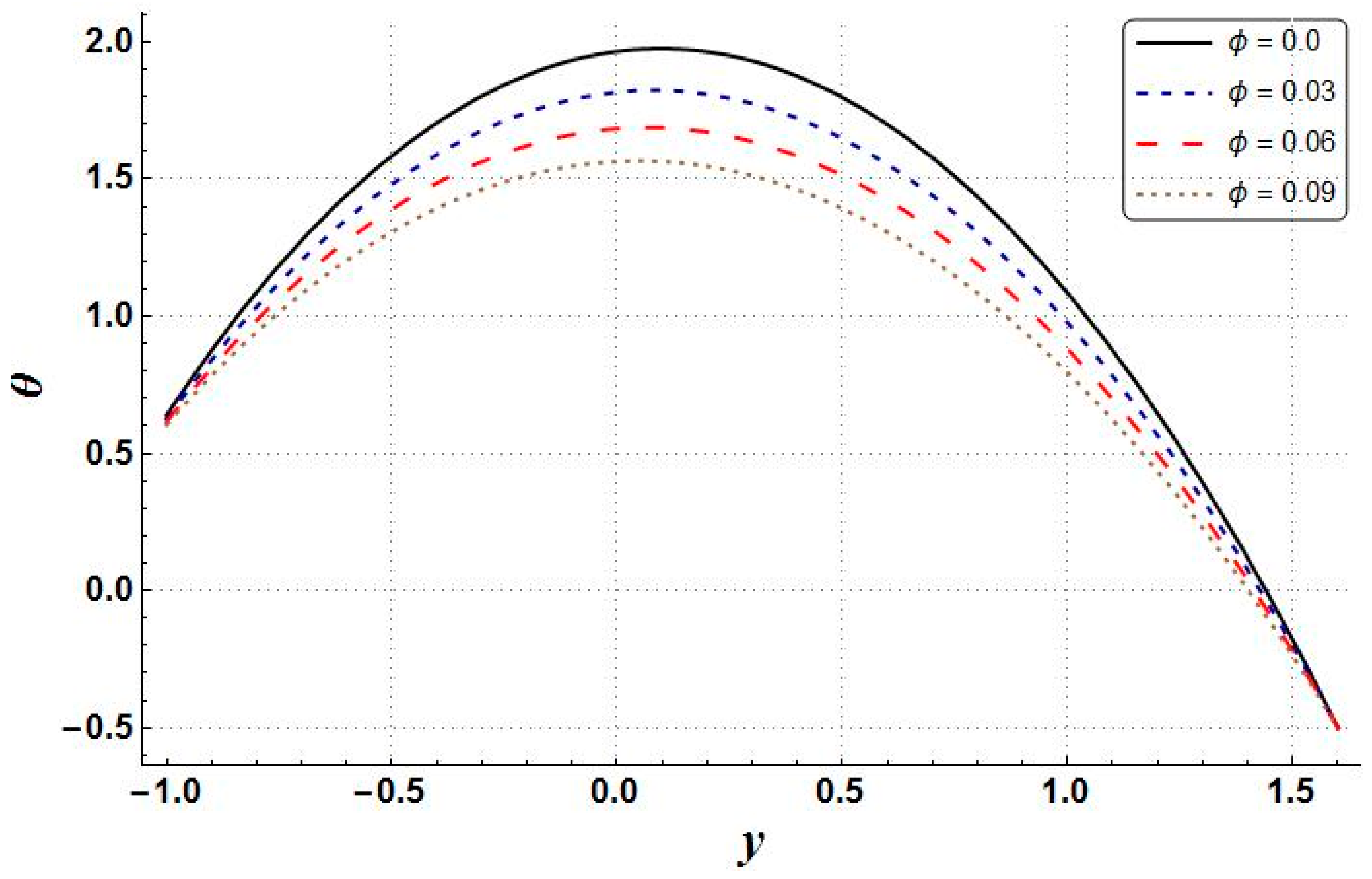
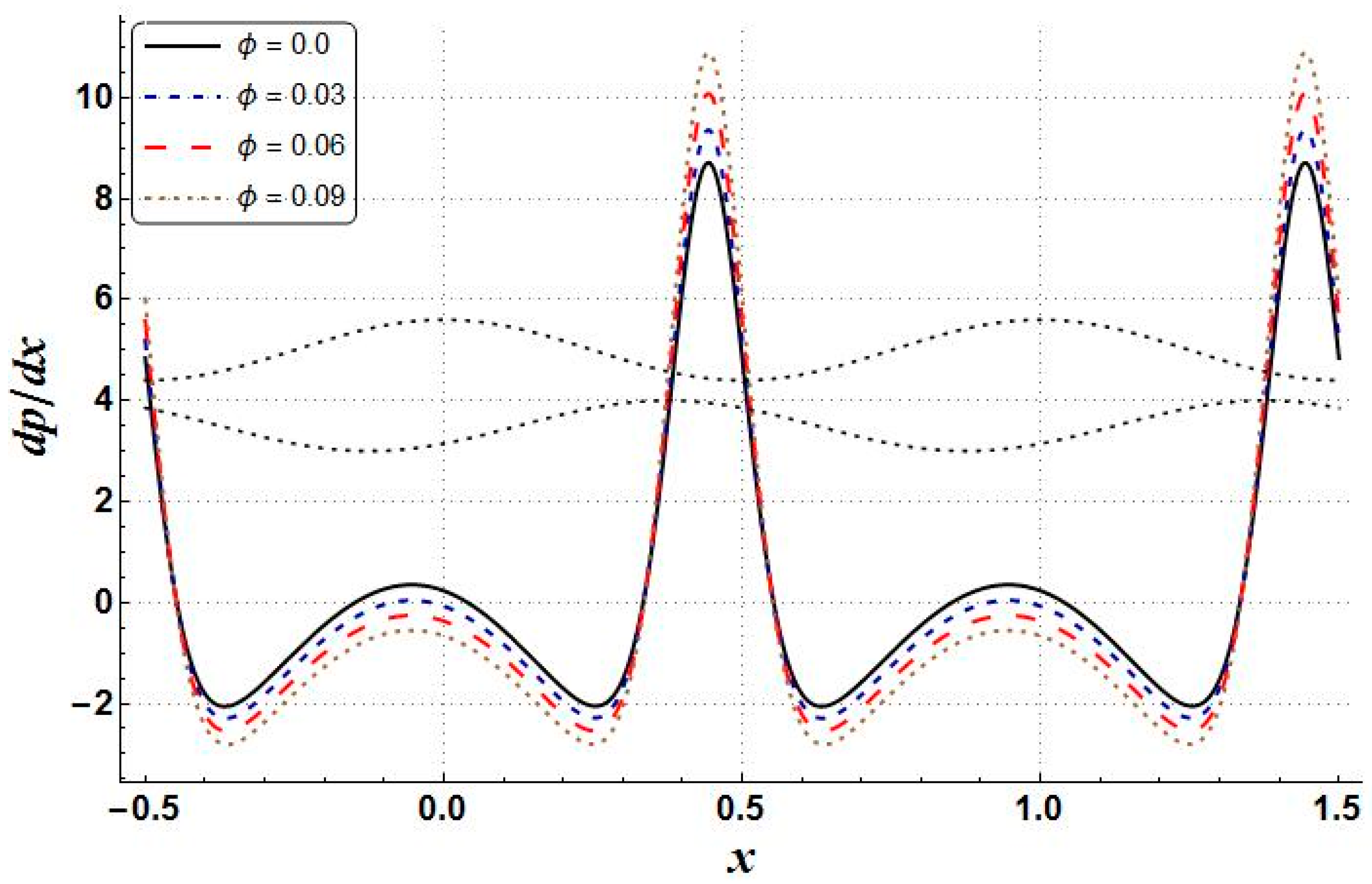
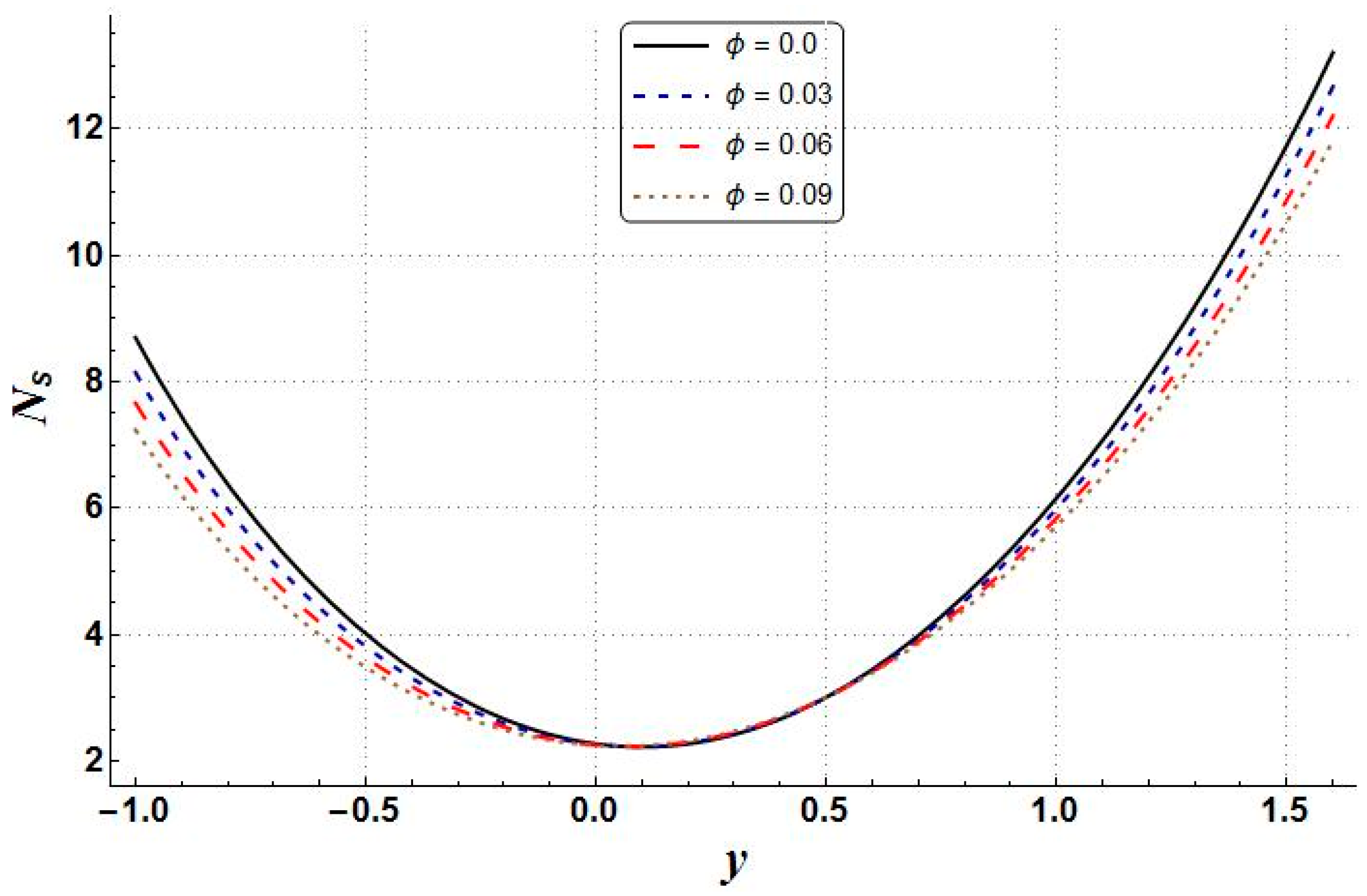
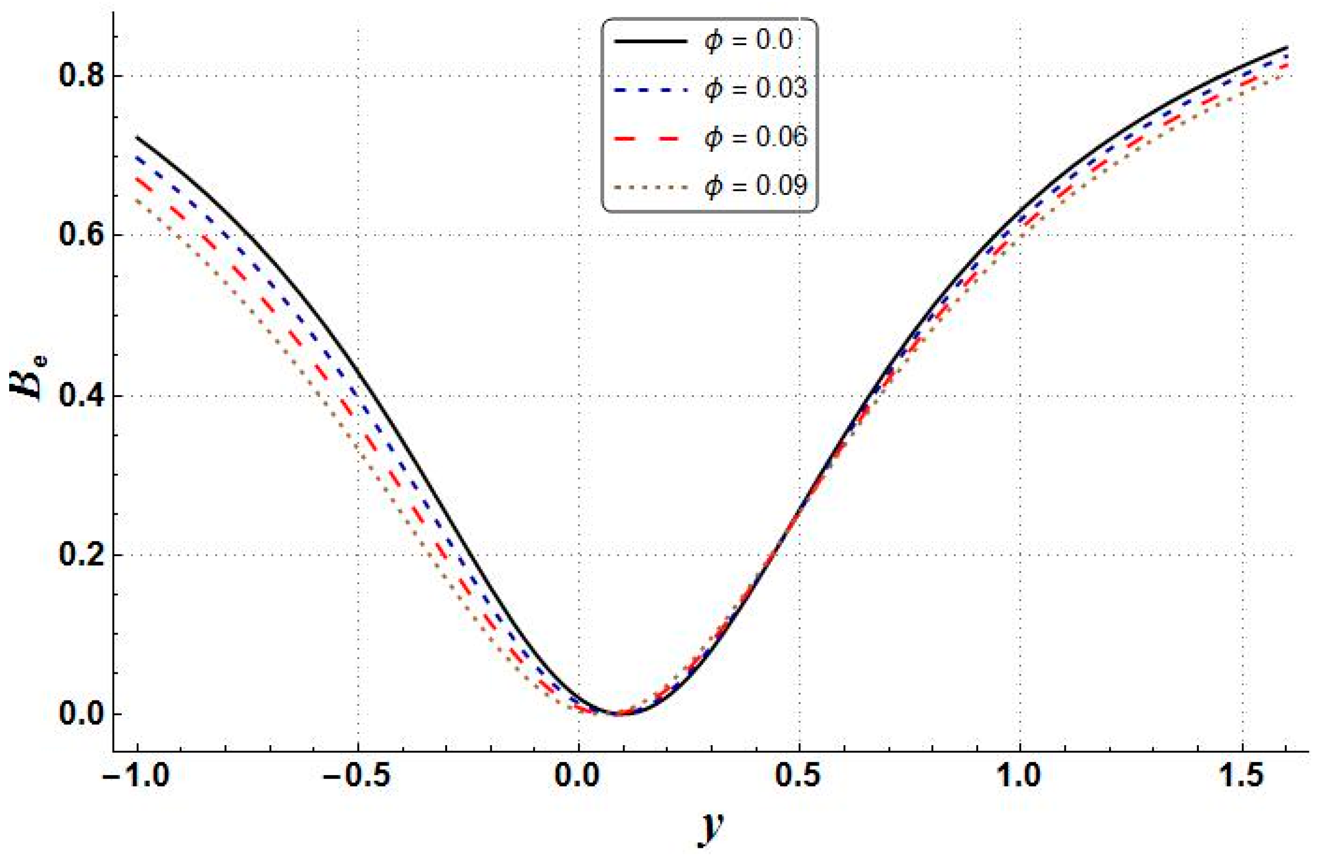
• The growth of nanoparticle volume fraction resulted in the reduction of temperature, entropy generation, velocity, pressure gradient, and Bejan number;
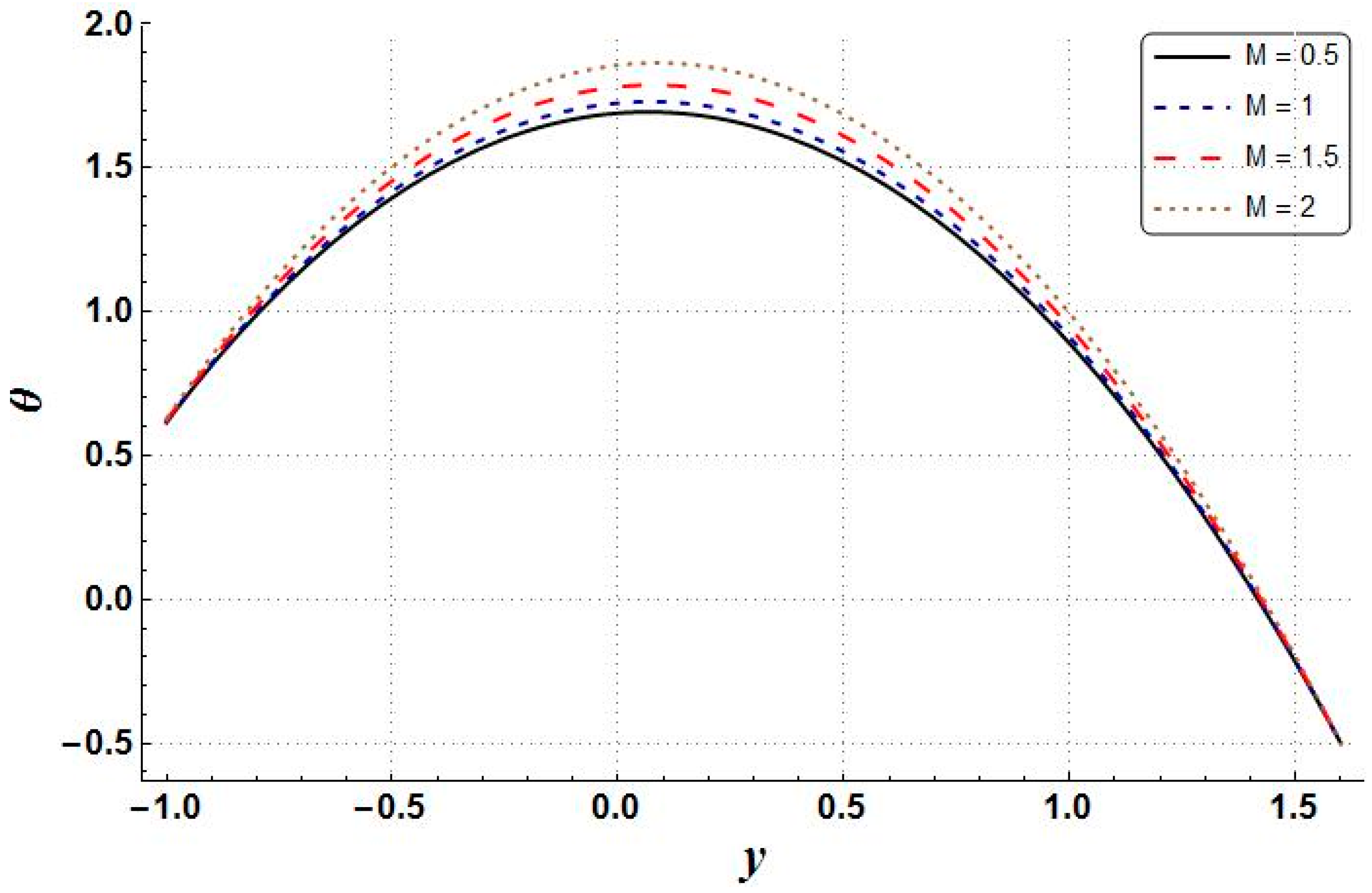
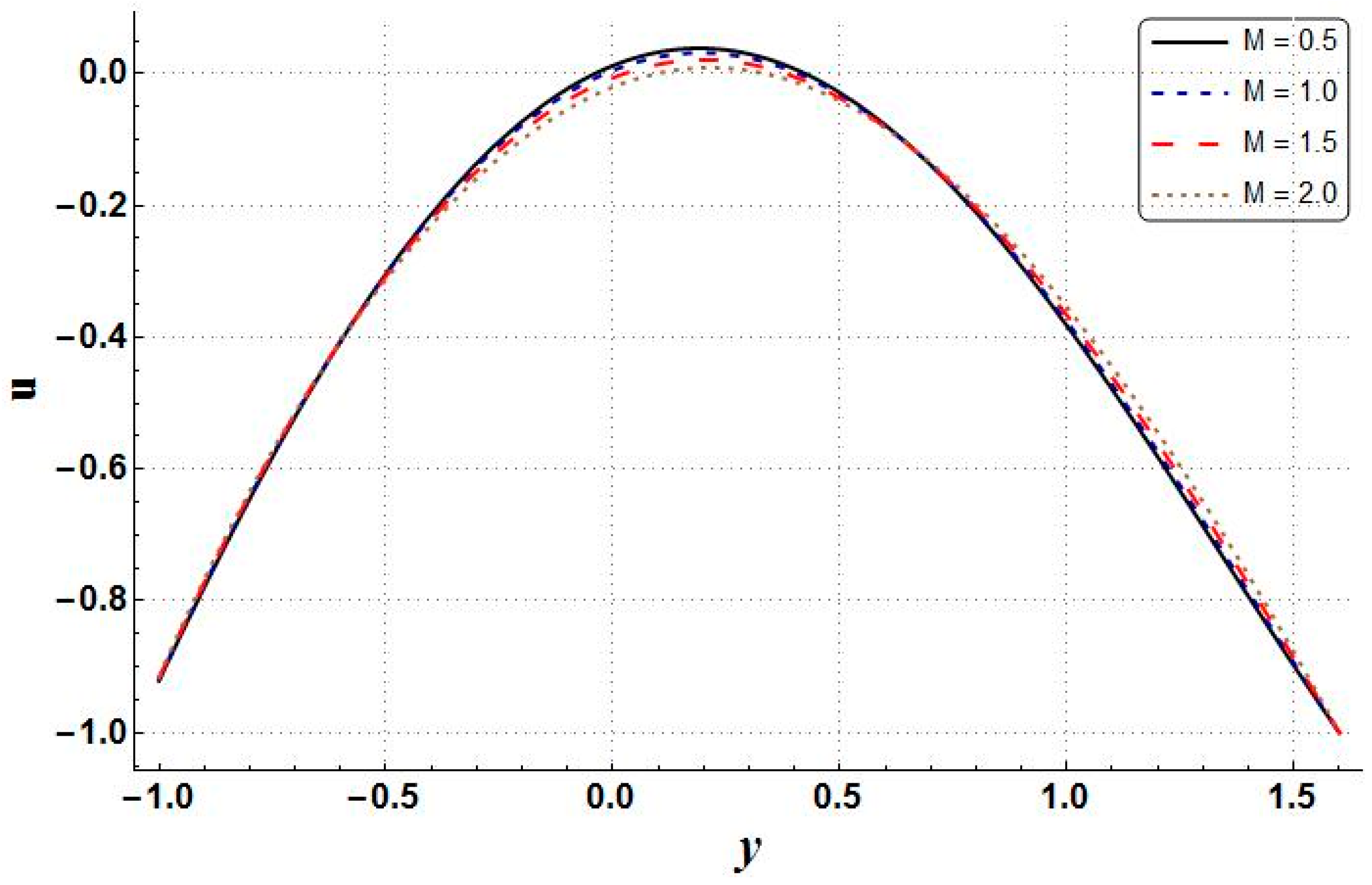
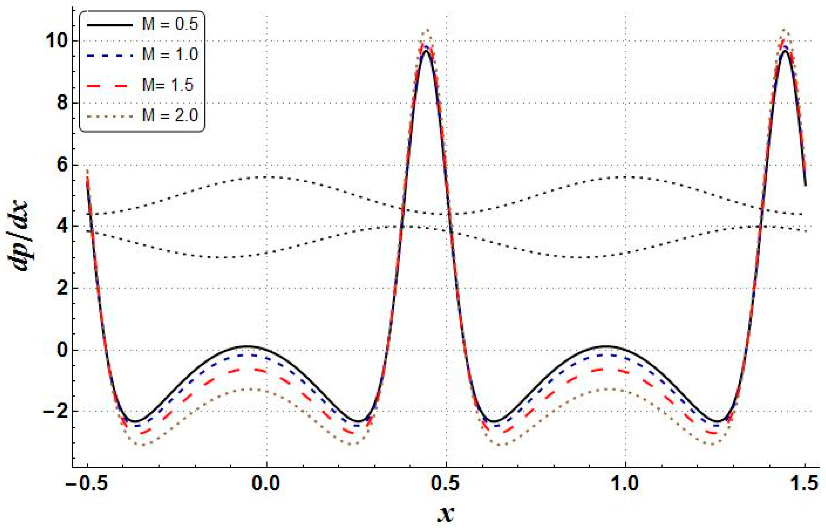
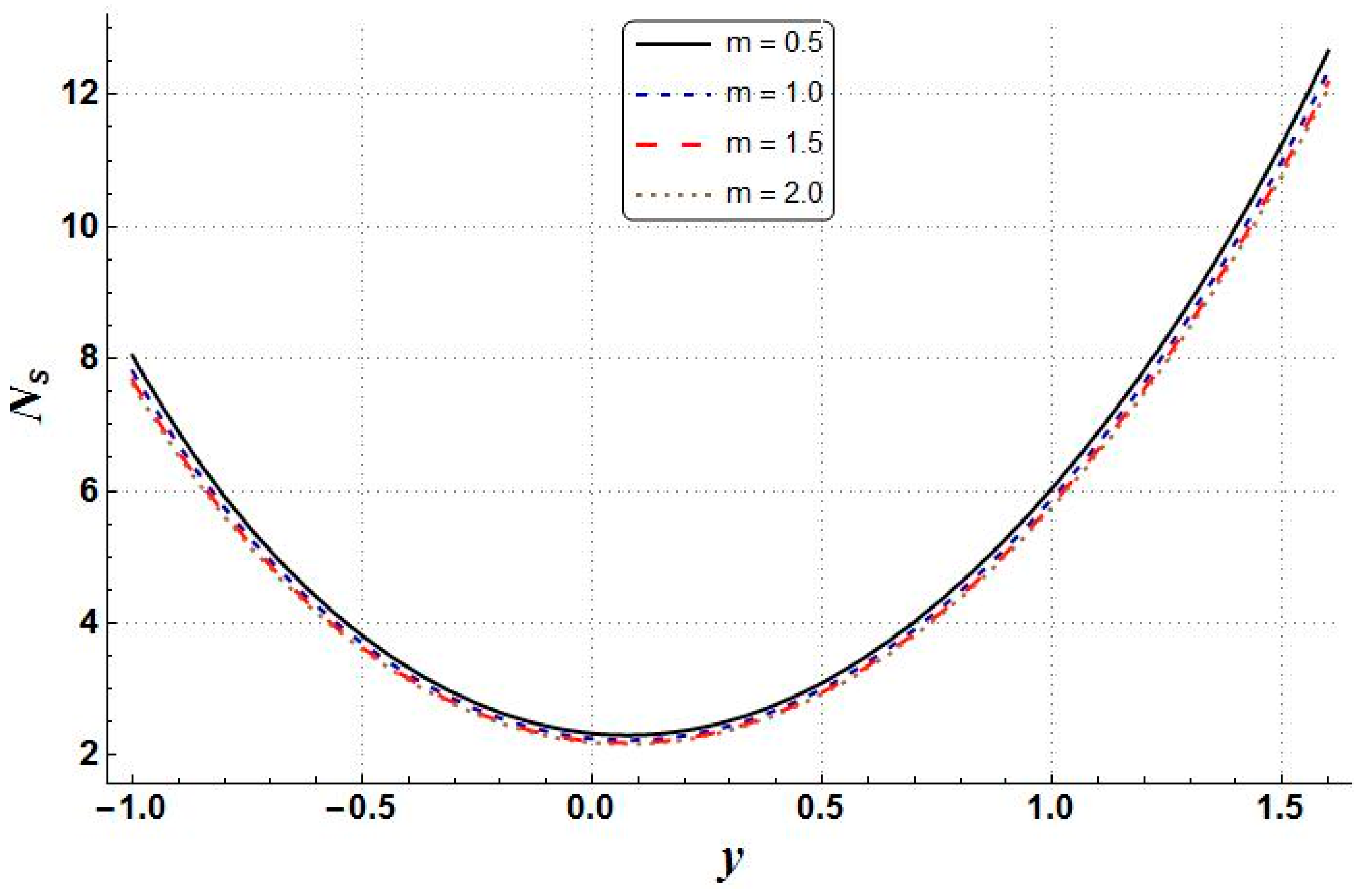
• Increases in the values of entropy generation, Bejan number, and temperature have been noted as being due to increasing values of Hartman number, whereas the velocity profile and pressure gradient behaved in quite the opposite way;
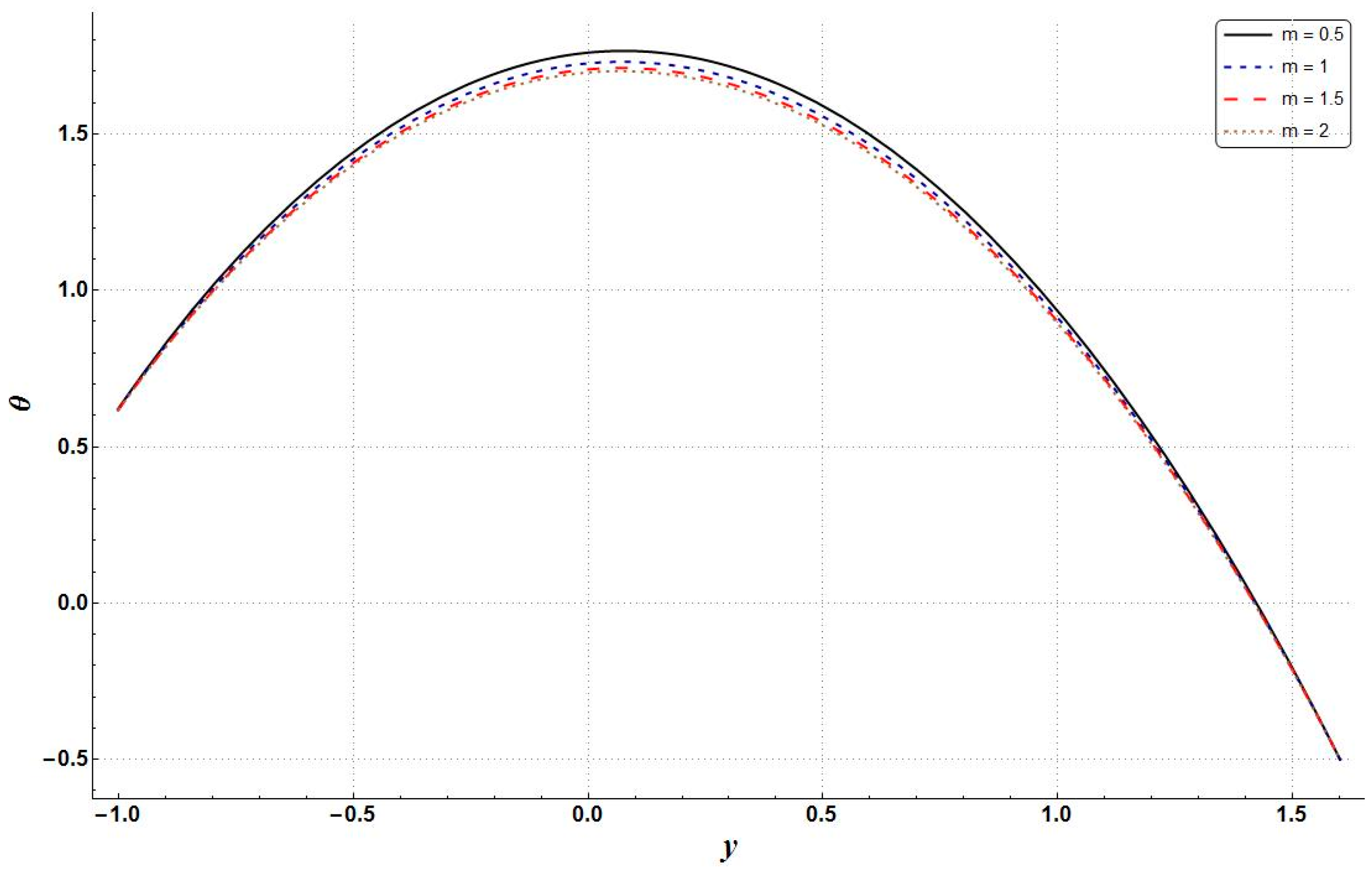
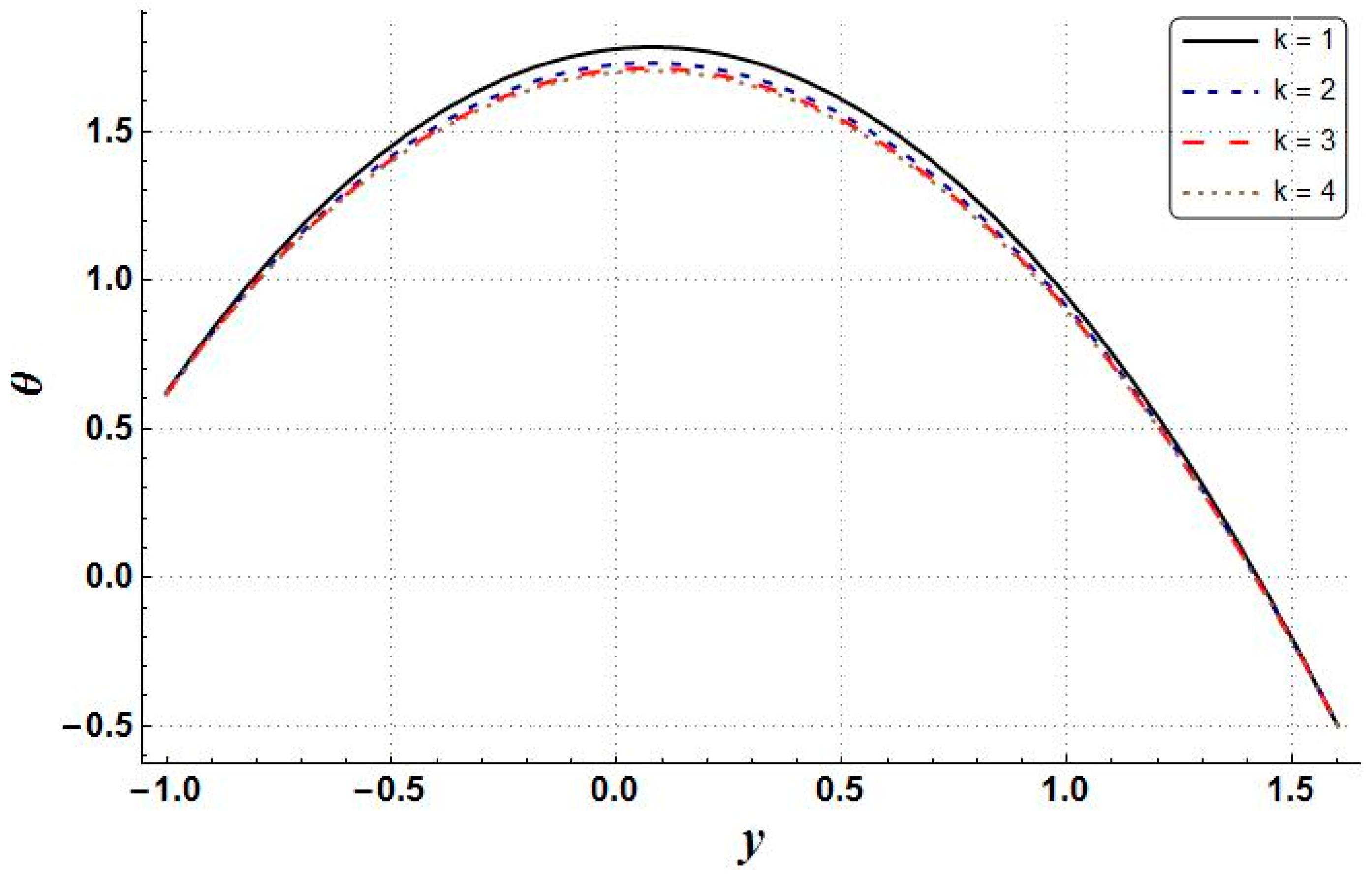
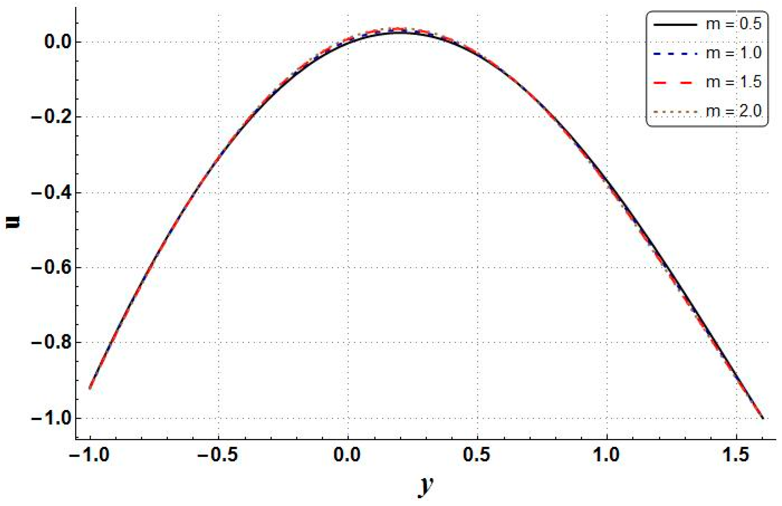
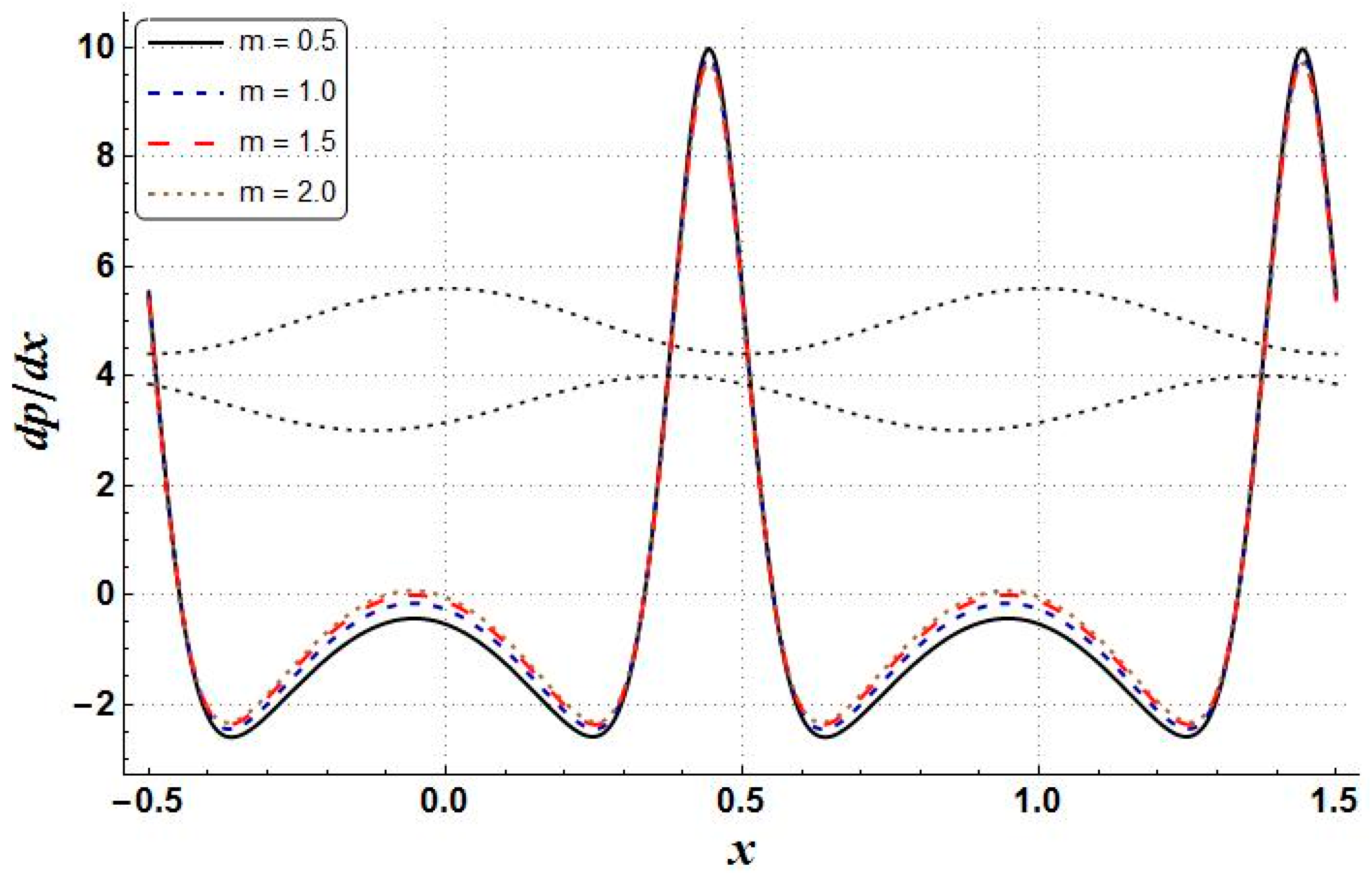
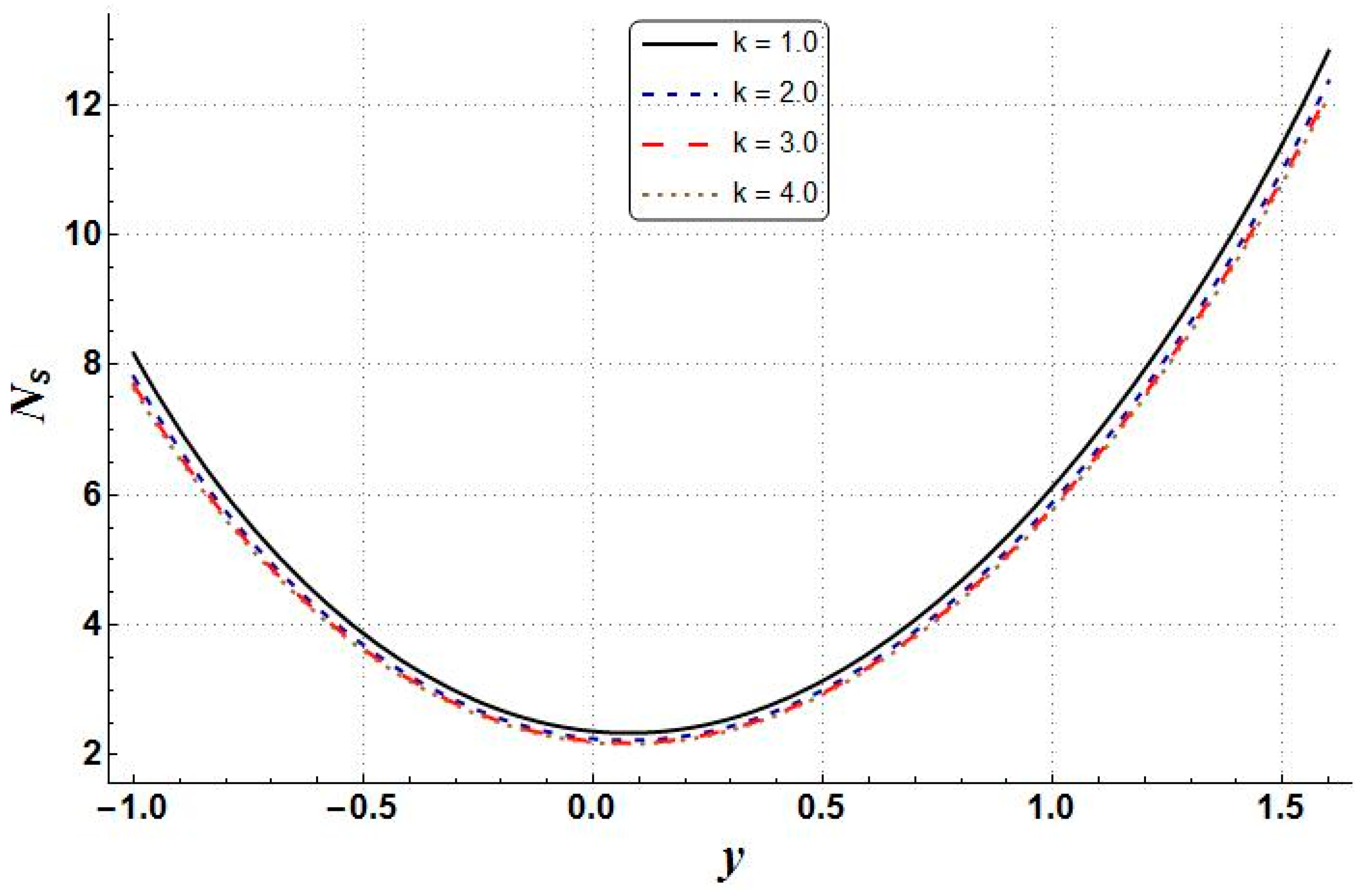
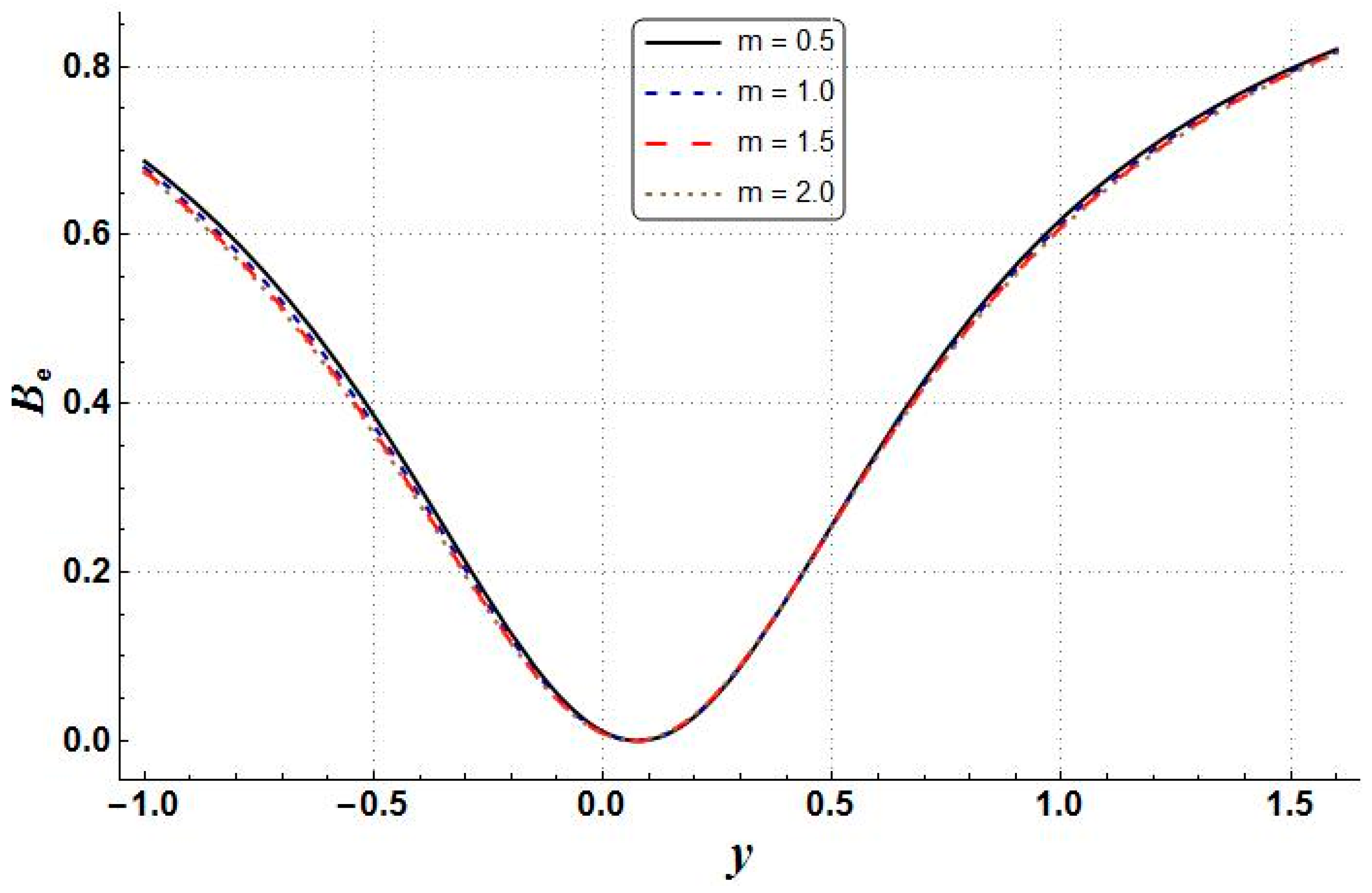
• Reductions in the entropy generation, temperature, and Bejan number were shown to be due to an increase in the Hall parameter, as shown by the relevant figures. However, the velocity of the nanofluid and pressure gradient increased;
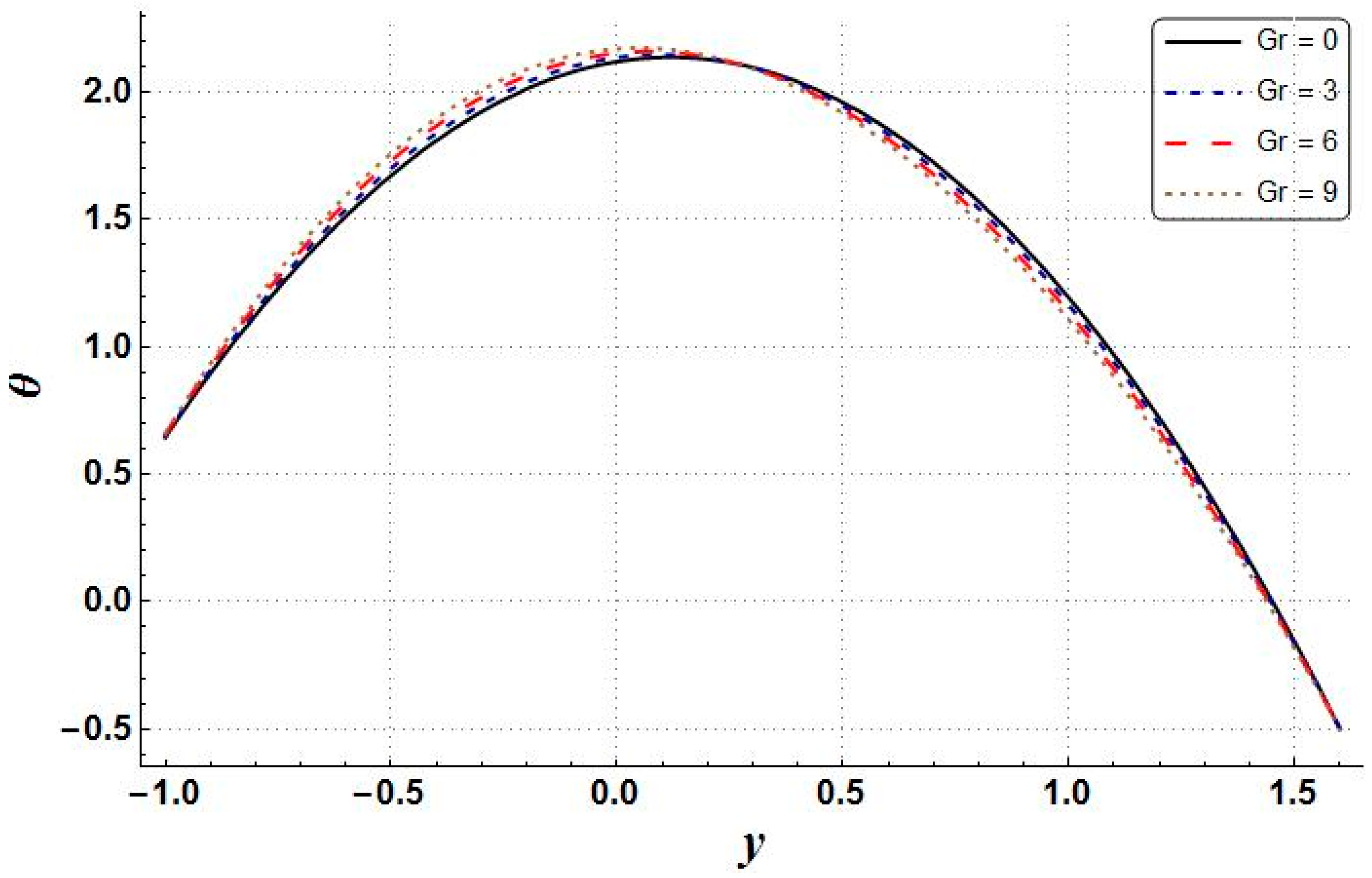
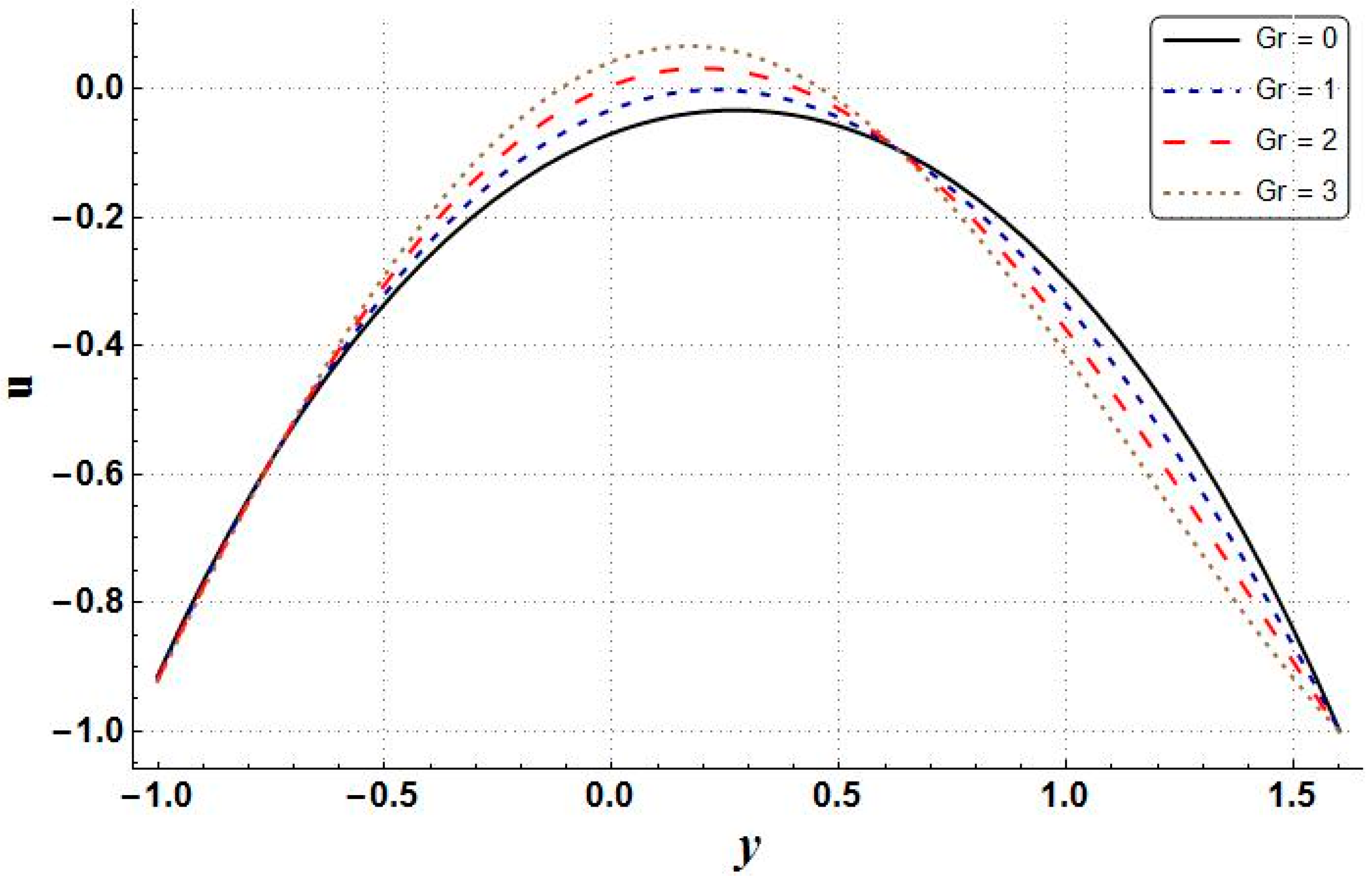
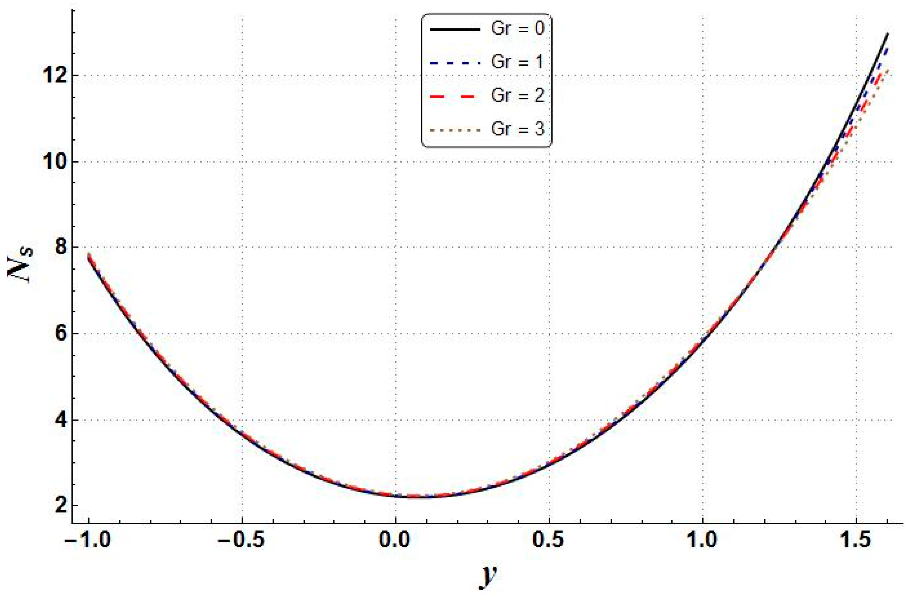
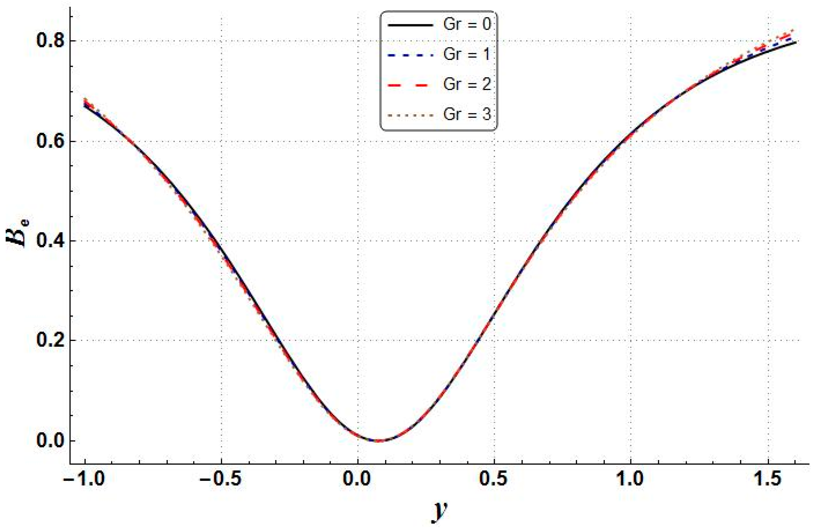
• The velocity, pressure gradient, and Bejan number showed an increasing trend with the increasing values of Grashof number;
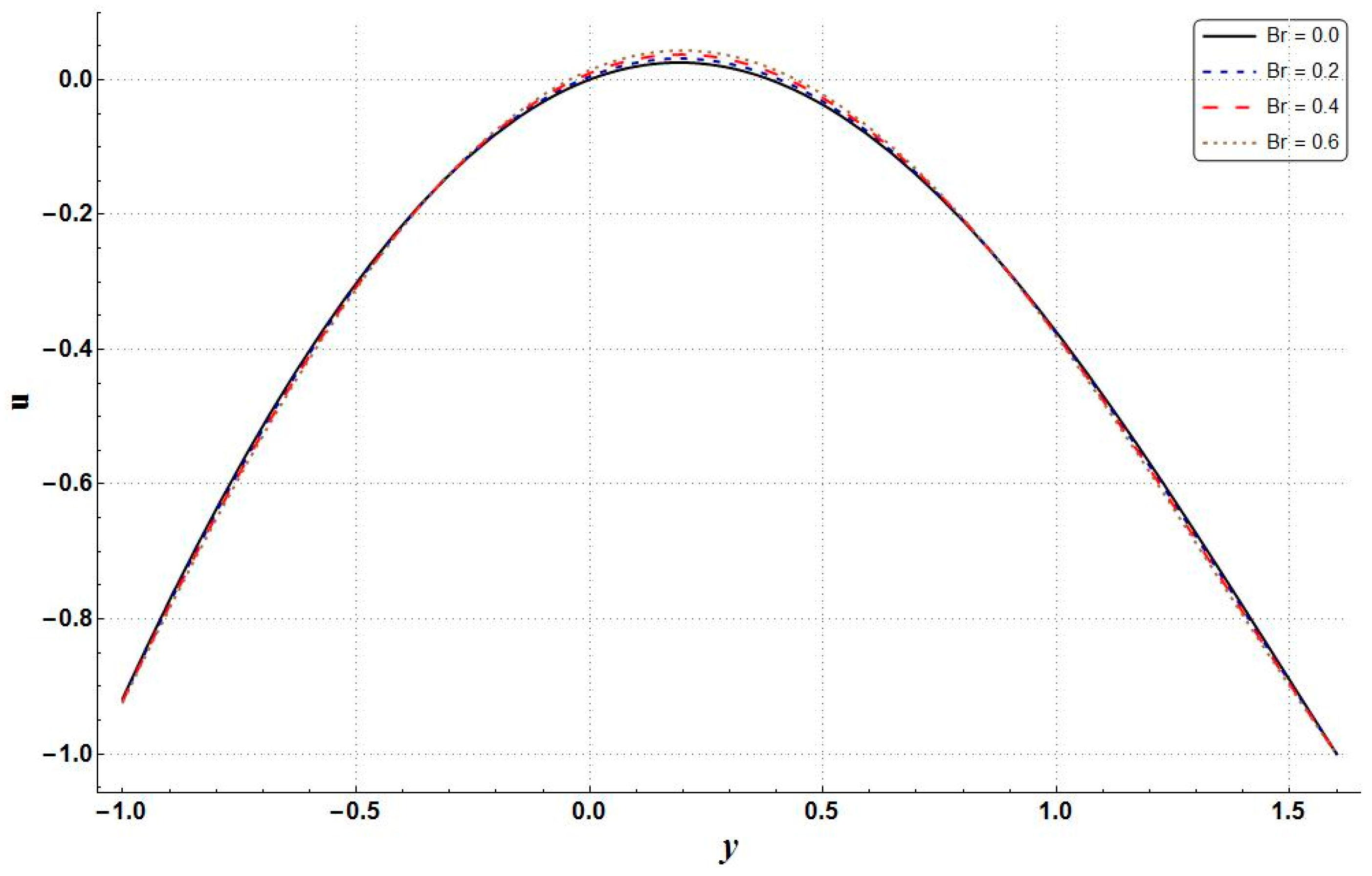
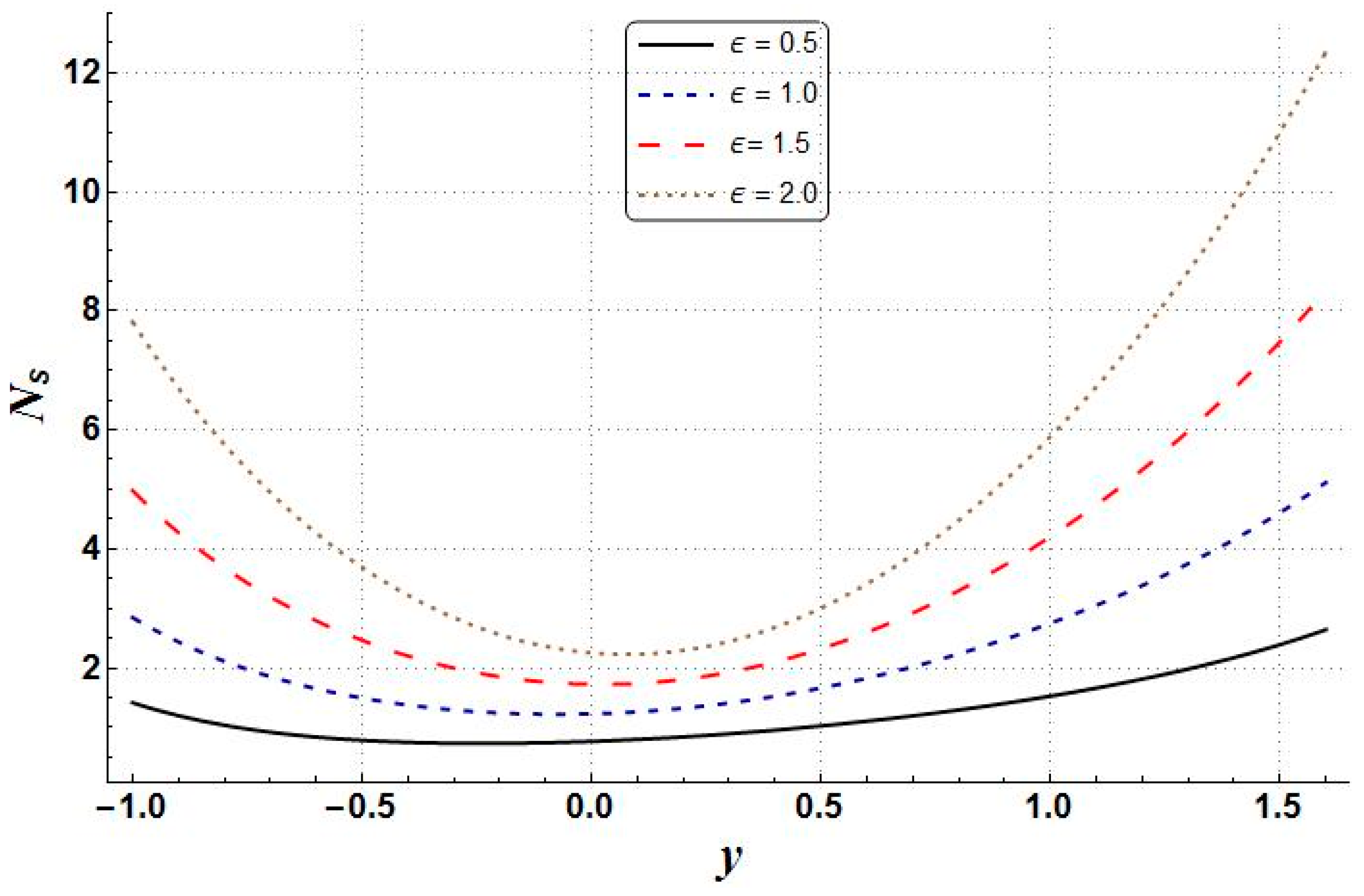
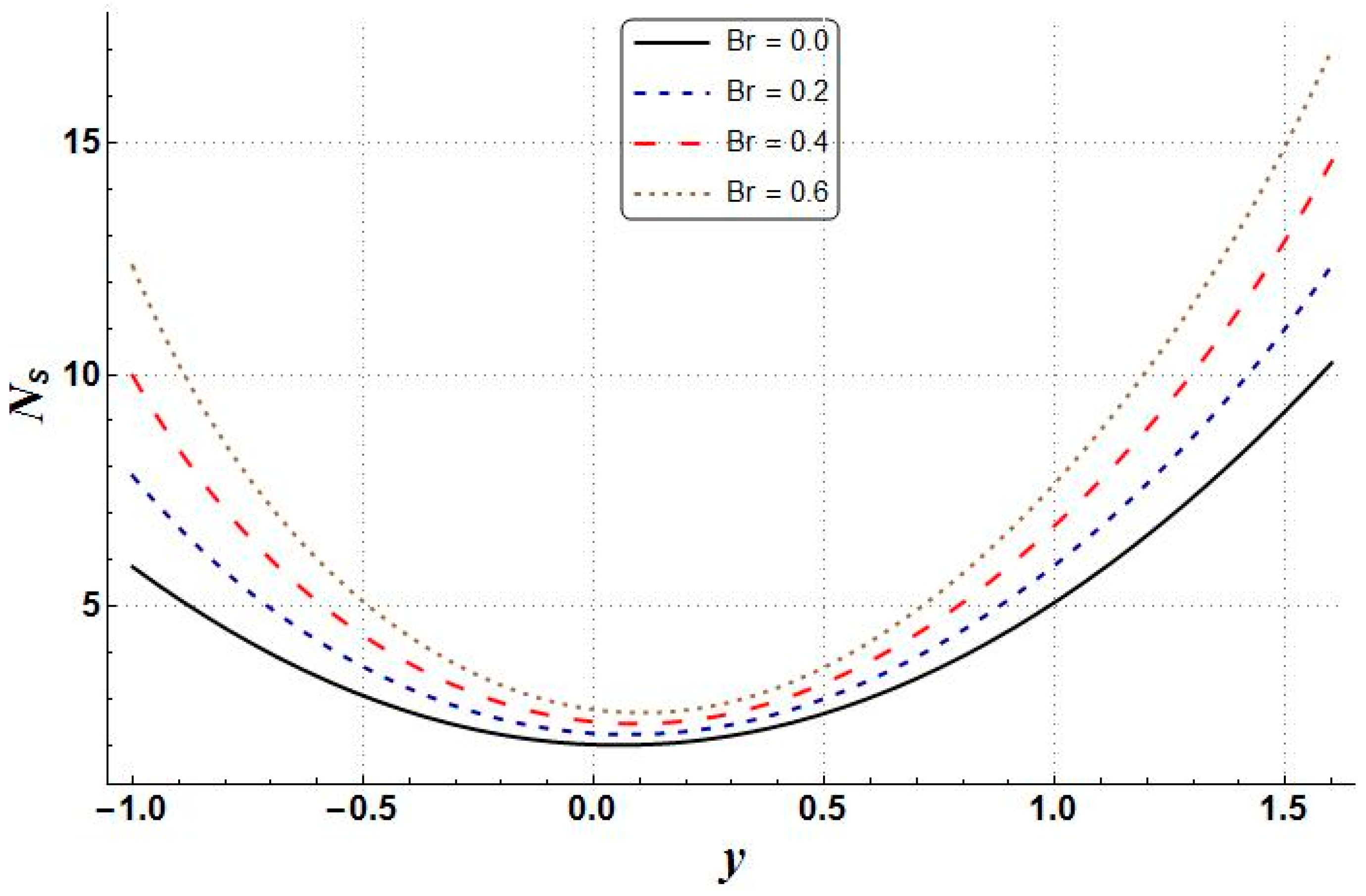
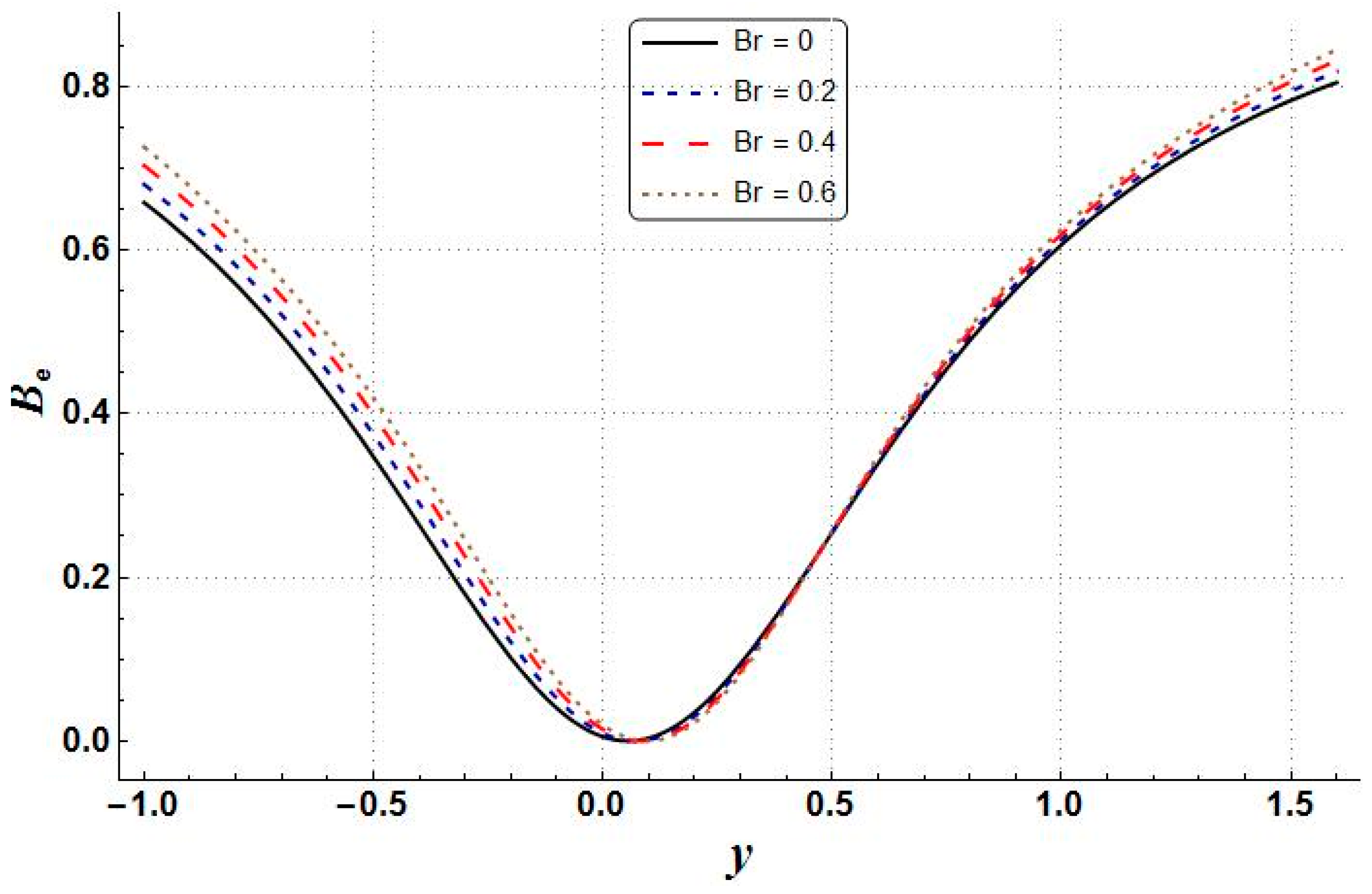
• The entropy generation, temperature, velocity, pressure gradient, and Bejan numbers increased with higher values of Brinkman number.

It is important to note that the investigated problem has certain limitations, due to the consideration of additional physical effects. The choice of physical parameters should be made in a manner such that motility disorder does not occur. For example, the occurrence of motility disorder during the food pumping process may tend towards either too fast or too slow peristalsis, which leads to problems with digestion, constipation, and bacterial overgrowth.

As a continuation of the above study, it is recommended that future research analyze the impact of variable thermal conductivity on the peristaltic flow of nanofluids, since thermal conductivities of fluids vary with large temperature fluctuations. Different types of nanoparticles (i.e., copper, silver, gold, alumina, etc.) could be used in these analyses, with any base fluid. A comparison of results for different nanoparticles could also be conducted to facilitate future research in the field. In addition, considering the importance of advancements in hybrid nanofluids (Cu-TiO2/H₂O), one could study the peristaltic flow of a hybrid nanofluid under the influence of an applied magnetic field, with velocity and thermal slip boundary conditions. In such a situation, various nanoparticles are combined within a base fluid to achieve the desired thermal characteristics. The Lorentz force arising due to the applied magnetic field can be computed using Maxwell’s equations. The resulting system could be reduced using the lubrication approach and solved numerically via the built-in NDSolver in Mathematica.

References

1. Latham, T.W. Fluid Motion in a Peristaltic Pump. Master’s Thesis, Massachusetts Institute of Technology, Cambridge, MA, USA, 1966. [Google Scholar]
2. Shapiro, A.H.; Jaffrin, M.Y.; Weinberg, S.L. Peristaltic pumping with long wavelengths at low Reynolds number. J. Fluid Mech. 1969, 37, 799–825. [Google Scholar] [CrossRef]
3. Lew, S.H.; Fung, Y.C.; Lowenstein, C.B. Peristaltic carrying and mixing of chyme. J. Biomech. 1971, 4, 297–315. [Google Scholar] [CrossRef] [PubMed]
4. Chakraborty, S. Augmentation of peristaltic micro-flows through electro-osmotic mechanisms. J. Phys. D 2006, 39, 5356–5363. [Google Scholar] [CrossRef]
5. Riaz, A.; Ellahi, R.; Nadeem, S. Peristaltic transport of a Carreau fluid in a compliant rectangular duct. Alex. Eng. J. 2014, 53, 475–484. [Google Scholar] [CrossRef] [Green Version]
6. Abbasi, F.M.; Saba; Shehzad, S. A. Heat transfer analysis for peristaltic flow of Carreau-Yasuda fluid through a curved channel with radial magnetic field. Int. J. Heat Mass Transf. 2017, 115, 777–783. [Google Scholar] [CrossRef]
7. Hayat, T.; Ahmed, B.; Abbasi, F.M.; Alsaedi, A. Peristalsis of nanofluid through curved channel with Hall and Ohmic heating effects. J. Cent. South Univ. 2019, 26, 2543–2553. [Google Scholar] [CrossRef]
8. Rafiq, M.; Yasmin, H.; Hayat, T.; Alsaadi, F. Effect of Hall and ion-slip on the peristaltic transport of nanofluid: A biomedical application. Chin. J. Phys. 2019, 60, 208–227. [Google Scholar] [CrossRef]
9. Eldabe, N.T.; Moatimid, G.M.; Abouzeid, M.Y.; ElShekhipy, A.A.; Abdallah, N.F. A semianalytical technique for MHD peristalsis of pseudo plastic nanofluid with temperature-dependent viscosity: Application in drug delivery system. Heat Transf.-Asian Res. 2020, 49, 424–440. [Google Scholar] [CrossRef]
10. Choi, S.U.S.; Eastman, J.A. Enhancing thermal conductivity of fluids with nanoparticles. In Proceedings of the 1995 International mechanical engineering congress and exhibition, San Francisco, CA, USA, 12–17 November 1995; Argonne National Lab.: Argonne, IL, USA, 1995; pp. 12–17. [Google Scholar]
11. Choi, S.U.S. Enhancing thermal conductivity of fluid with nanofluids. In Developments and Applications of Non-Newtonian Flows; Siginer, D.A., Wang, H., Eds.; Argonne National Lab.: Argonne, IL, USA, 1995; Volume 66, pp. 99–105. [Google Scholar]
12. Xue, Q.Z. Model for thermal conductivity of carbon nanotube-based composites. Phys. B Condens. Matter 2005, 368, 302–307. [Google Scholar] [CrossRef]
13. Pankhurst, Q.A.; Connolly, J.; Jones, S.K.; Dobson, J. Applications of magnetic nanoparticles in biomedicine. J. Phy. D Appl. Phys. 2003, 36, R167–R181. [Google Scholar] [CrossRef]
14. Habibi, M.R.; Ghassemi, M.; Hamedi, M.H. Analysis of high gradient magnetic field effects on distribution of nanoparticles injected into pulsatile blood stream. J. Magn. Magn. Mater. 2012, 324, 1473–1482. [Google Scholar] [CrossRef]
15. Hayat, T.; Nisar, Z.; Ahmad, B.; Yasmin, H. Simultaneous effects of slip and wall properties on MHD peristaltic motion of nanofluid with Joule heating. J. Magn. Magn. Mater. 2015, 395, 48–58. [Google Scholar] [CrossRef]
16. Ebaid, A. Effects of magnetic field and wall slip conditions on the peristaltic transport of a Newtonian fluid in an asymmetric channel. Phys. Lett. A 2008, 372, 4493–4499. [Google Scholar] [CrossRef]
17. Abbasi, F.M.; Hayat, T.; Ahmad, B. Peristalsis of silver-water nanofluid in the presence of Hall and Ohmic heating effects: Application in drug delivery. J. Mol. Liq. 2015, 207, 248–255. [Google Scholar] [CrossRef]
18. Bejan, A. A study of entropy generation in fundamental convective heat transfer. ASME J. Heat Transf. 1979, 101, 718–725. [Google Scholar] [CrossRef]
19. Bejan, A. Entropy Generation Minimization; CRC Press: New York, NY, USA, 1996. [Google Scholar]
20. Hijleh, B.A.; Abu-Qudais, M.; Abu-Nada, E. Numerical prediction of entropy generation due to natural convection from a horizontal cylinder. Energy 1999, 24, 327–333. [Google Scholar] [CrossRef]
21. Ranjit, N.K.; Shit, G.C. Entropy generation on electro-osmotic flow pumping by a uniform peristaltic wave under magnetic environment. Energy 2017, 128, 649–660. [Google Scholar] [CrossRef]
22. Al-Hadhrami, A.K.; Elliott, L.; Ingham, D.B. A new model for viscous dissipation in porous media across a range of permeability values. Transp. Porous Media 2003, 53, 117–122. [Google Scholar] [CrossRef]
23. Hayat, T.; Abbasi, F.M.; Ahmad, B.; Chen, G.-Q. Slip effects on mixed convective peristaltic transport of copper-water nanofluid in an inclined channel. PLoS ONE 2014, 9, e105440. [Google Scholar] [CrossRef] [PubMed]
24. Bazdar, H.; Toghraie, D.; Pourfattah, F.; Akbari, O.A.; Nguyen, H.M.; Asadi, A. Numerical investigation of turbulent flow and heat transfer of nanofluid inside a wavy microchannel with different wavelengths. J. Therm. Anal. Calorim. 2020, 139, 2365–2380. [Google Scholar] [CrossRef]
25. Arasteh, H.; Mashayekhi, R.; Goodarzi, M.; Motaharpour, S.H.; Dahari, M.; Toghraie, D. Heat and fluid flow analysis of metal foam embedded in a double-layered sinusoidal heat sink under local thermal non-equilibrium condition using nanofluid. J. Therm. Anal. Calorim. 2019, 138, 1461–1476. [Google Scholar] [CrossRef]
26. Khodabandeh, E.; Rozati, S.A.; Joshaghani, M.; Akbari, O.A.; Akbari, S.; Toghraie, D. Thermal performance improvement in water nanofluid/GNP–SDBS in novel design of double-layer microchannel heat sink with sinusoidal cavities and rectangular ribs. J. Therm. Anal. Calorim. 2019, 136, 1333–1345. [Google Scholar] [CrossRef]
27. Boroomandpour, A.; Toghraie, D.; Hashemian, M. A comprehensive experimental investigation of thermal conductivity of a ternary hybrid nanofluid containing MWCNTs-titania-zinc oxide/water-ethylene glycol (80:20). Synth. Met. 2020, 268, 116501. [Google Scholar] [CrossRef]
28. Akbari, S.; Faghiri, S.; Poureslami, P.; Hosseinzadeh, K.; Shafii, M.B. Analytical solution of non-Fourier heat conduction in a 3-D hollow sphere under time-space varying boundary conditions. Heliyon 2022, 8, e12496. [Google Scholar] [CrossRef]
29. Faghiri, S.; Akbari, S.; Shafii, M.B.; Hosseinzadeh, K. Hydrothermal analysis of non-Newtonian fluid flow (blood) through the circular tube under prescribed non-uniform wall heat flux. Theor. Appl. Mech. Lett. 2022, 12, 100360. [Google Scholar] [CrossRef]
30. Gulzar, M.M.; Aslam, A.; Waqas, M.; Javed, M.A.; Hosseinzadeh, K. A nonlinear mathematical analysis for magneto-hyperbolic-tangent liquid featuring simultaneous aspects of magnetic field, heat source and thermal stratification. Appl. Nanosci. 2020, 10, 4513–4518. [Google Scholar] [CrossRef]
31. Ramesh, K. Influence of heat and mass transfer on peristaltic flow of a couple stress fluid through porous medium in the presence of inclined magnetic field in an inclined asymmetric channel. J. Mol. Liq. 2016, 71, 219–256. [Google Scholar] [CrossRef]
32. Turkyilmazoglu, M. Nanofluid flow and heat transfer due to a rotating disk. Comput. Fluids 2014, 94, 139–146. [Google Scholar] [CrossRef]
Figure 1. Peristalsis flow geometry.
Mathematics 11 00458 g001
Figure 2. Influence on θ through changing values of ϕ , where γ = π 4 , x = 0 , G r = 2 , α = π 4 ,   M = 1 , k = 2 , a = 0.6 , m = 1 , d = 0.7 , B r = 0.2 , b = 0.5 , = 2 , η = 0.8 .
Mathematics 11 00458 g002
Figure 3. Influence on θ through changing values of M , where γ = π 4 , x = 0 , G r = 2 ,   α = π 4 , ϕ = 0.05 , k = 2 , a = 0.6 , m = 1 , d = 0.7 , B r = 0.2 , b = 0.5 , = 2 , η = 0.8 .
Mathematics 11 00458 g003
Figure 4. Influence on θ through changing values of m , where γ = π 4 , x = 0 , G r = 2 ,   α = π 4 , ϕ = 0.05 , k = 2 , a = 0.6 , M = 1 , d = 0.7 , B r = 0.2 , b = 0.5 , = 2 , η = 0.8 .
Mathematics 11 00458 g004
Figure 5. Influence on θ through changing values of k , where γ = π 4 , x = 0 , G r = 2 ,   α = π 4 , ϕ = 0.05 , m = 1 , a = 0.6 , M = 1 , d = 0.7 , B r = 0.2 , b = 0.5 , = 2 , η = 0.8 .
Mathematics 11 00458 g005
Figure 6. Influence on θ through changing values of , where γ = π 4 , x = 0 , G r = 2 ,   α = π 4 , ϕ = 0.05 , k = 2 , a = 0.6 , M = 1 , d = 0.7 , B r = 0.2 , b = 0.5 , m = 1 , η = 0.8 .
Mathematics 11 00458 g006
Figure 7. Influence on θ through changing values of B r , where γ = π 4 , x = 0 , G r = 2 ,   α = π 4 , ϕ = 0.05 , k = 2 , a = 0.6 , M = 1 , d = 0.7 , m = 1 , b = 0.5 , = 2 , η = 0.8 .
Mathematics 11 00458 g007
Figure 8. Influence on θ through changing values of G r , where γ = π 4 , x = 0 , B r = 0.2 ,   α = π 4 , ϕ = 0.05 , k = 0.2 , a = 0.6 , M = 1 , d = 0.7 , m = 1 , b = 0.5 , = 2 , η = 0.8 .
Mathematics 11 00458 g008
Figure 9. Influence on u through changing values of ϕ , where γ = π 4 , x = 0 , G r = 2 , α = π 4 ,   M = 1 , k = 2 , a = 0.6 , m = 1 , d = 0.7 , B r = 0.2 , b = 0.5 , = 2 , η = 0.8 .
Mathematics 11 00458 g009
Figure 10. Influence on u through changing values of M , where γ = π 4 , x = 0 , G r = 2 ,   α = π 4 , ϕ = 0.05 , k = 2 , a = 0.6 , m = 1 , d = 0.7 , B r = 0.2 , b = 0.5 , = 2 , η = 0.8 .
Mathematics 11 00458 g010
Figure 11. Influence on u through changing values of m , where γ = π 4 , x = 0 , G r = 2 ,   α = π 4 , ϕ = 0.05 , k = 2 , a = 0.6 , M = 1 , d = 0.7 , B r = 0.2 , b = 0.5 , = 2 , η = 0.8 .
Mathematics 11 00458 g011
Figure 12. Influence on u through changing values of k , where γ = π 4 , x = 0 , G r = 2 ,   α = π 4 , ϕ = 0.05 , m = 1 , a = 0.6 , M = 1 , d = 0.7 , B r = 0.2 , b = 0.5 , = 2 , η = 0.8 .
Mathematics 11 00458 g012
Figure 13. Influence on u through changing values of , where γ = π 4 , x = 0 , G r = 2 ,   α = π 4 , ϕ = 0.05 , k = 2 , a = 0.6 , M = 1 , d = 0.7 , B r = 0.2 , b = 0.5 , m = 1 , η = 0.8 .
Mathematics 11 00458 g013
Figure 14. Influence on u through changing values of B r , where γ = π 4 , x = 0 , G r = 2 ,   α = π 4 , ϕ = 0.05 , k = 2 , a = 0.6 , M = 1 , d = 0.7 , m = 1 , b = 0.5 , = 2 , η = 0.8 .
Mathematics 11 00458 g014
Figure 15. Influence on u through changing values of G r , where γ = π 4 , x = 0 , B r = 0.2 ,   α = π 4 , ϕ = 0.05 , k = 2 , a = 0.6 , M = 1 , d = 0.7 , m = 1 , b = 0.5 , = 2 , η = 0.8 .
Mathematics 11 00458 g015
Figure 16. Influence on d p d x through changing values of ϕ , where γ = π 4 , x = 0 , G r = 2 ,   α = π 4 , M = 1 , k = 2 , a = 0.6 , m = 1 , d = 0.7 , B r = 0.2 , b = 0.5 , = 2 , η = 0.8 .
Mathematics 11 00458 g016
Figure 17. Influence on d p d x through changing values of M , where γ = π 4 , x = 0 , G r = 2 ,   α = π 4 , ϕ = 0.05 , k = 2 , a = 0.6 , m = 1 , d = 0.7 , B r = 0.2 , b = 0.5 , = 2 , η = 0.8 .
Mathematics 11 00458 g017
Figure 18. Influence on d p d x through changing values of m , where γ = π 4 , x = 0 , G r = 2 ,   α = π 4 , ϕ = 0.05 , k = 2 , a = 0.6 , M = 1 , d = 0.7 , B r = 0.2 , b = 0.5 , = 2 , η = 0.8 .
Mathematics 11 00458 g018
Figure 19. Influence on d p d x through changing values of k , where γ = π 4 , x = 0 , G r = 2 ,   α = π 4 , ϕ = 0.05 , m = 1 , a = 0.6 , M = 1 , d = 0.7 , B r = 0.2 , b = 0.5 , = 2 , η = 0.8 .
Mathematics 11 00458 g019
Figure 20. Influence on d p d x through changing values of , where γ = π 4 , x = 0 , G r = 2 ,   α = π 4 , ϕ = 0.05 , k = 2 , a = 0.6 , M = 1 , d = 0.7 , B r = 0.2 , b = 0.5 , m = 1 , η = 0.8 .
Mathematics 11 00458 g020
Figure 21. Influence on d p d x through changing values of G r , where γ = π 4 , x = 0 , B r = 0.2 ,   α = π 4 , ϕ = 0.05 , k = 2 , a = 0.6 , M = 1 , d = 0.7 , m = 1 , b = 0.5 , = 2 , η = 0.8 .
Mathematics 11 00458 g021
Figure 22. Influence on d p d x through changing values of B r , where γ = π 4 , x = 0 , G r = 2 ,   α = π 4 , ϕ = 0.05 , k = 2 , a = 0.6 , M = 1 , d = 0.7 , m = 1 , b = 0.5 , = 2 , η = 0.8 .
Mathematics 11 00458 g022
Figure 23. Influence on N S through changing values of ϕ , where γ = π 4 , x = 0 , G r = 2 ,   α = π 4 , M = 1 , k = 2 , a = 0.6 , m = 1 , d = 0.7 , B r = 0.2 , b = 0.5 , = 2 , η = 0.8 .
Mathematics 11 00458 g023
Figure 24. Influence on N S through changing values of M , where γ = π 4 , x = 0 , G r = 2 ,   α = π 4 , ϕ = 0.05 , k = 2 , a = 0.6 , m = 1 , d = 0.7 , B r = 0.2 , b = 0.5 , = 2 , η = 0.8 .
Mathematics 11 00458 g024
Figure 25. Influence on N S through changing values of m , where γ = π 4 , x = 0 , G r = 2 ,   α = π 4 , ϕ = 0.05 , k = 2 , a = 0.6 , M = 1 , d = 0.7 , B r = 0.2 , b = 0.5 , = 2 , η = 0.8 .
Mathematics 11 00458 g025
Figure 26. Influence on N S through changing values of , where γ = π 4 , x = 0 , G r = 2 ,   α = π 4 , ϕ = 0.05 , k = 2 , a = 0.6 , M = 1 , d = 0.7 , B r = 0.2 , b = 0.5 , m = 1 , η = 0.8 .
Mathematics 11 00458 g026
Figure 27. Influence on N S through changing values of k , where γ = π 4 , x = 0 , G r = 2 ,   α = π 4 , ϕ = 0.05 , m = 1 , a = 0.6 , M = 1 , d = 0.7 , B r = 0.2 , b = 0.5 , = 2 , η = 0.8 .
Mathematics 11 00458 g027
Figure 28. Influence on N S through changing values of G r , where γ = π 4 , x = 0 , B r = 0.2 ,   α = π 4 , ϕ = 0.05 , k = 2 , a = 0.6 , M = 1 , d = 0.7 , m = 1 , b = 0.5 , = 2 , η = 0.8 .
Mathematics 11 00458 g028
Figure 29. Influence on N S through changing values of B r , where γ = π 4 , x = 0 , G r = 2 ,   α = π 4 , ϕ = 0.05 , k = 2 , a = 0.6 , M = 1 , d = 0.7 , m = 1 , b = 0.5 , = 2 , η = 0.8 .
Mathematics 11 00458 g029
Figure 30. Influence on B e through changing values of ϕ , where γ = π 4 , x = 0 , G r = 2 ,   α = π 4 , M = 1 , k = 2 , a = 0.6 , m = 1 , d = 0.7 , B r = 0.2 , b = 0.5 , = 2 , η = 0.8 .
Mathematics 11 00458 g030
Figure 31. Influence on B e through changing values of M , where γ = π 4 , x = 0 , G r = 2 ,   α = π 4 , ϕ = 0.05 , k = 2 , a = 0.6 , m = 1 , d = 0.7 , B r = 0.2 , b = 0.5 , = 2 , η = 0.8 .
Mathematics 11 00458 g031
Figure 32. Influence on B e through changing values of m , where γ = π 4 , x = 0 , G r = 2 ,   α = π 4 , ϕ = 0.05 , k = 2 , a = 0.6 , M = 1 , d = 0.7 , B r = 0.2 , b = 0.5 , = 2 , η = 0.8 .
Mathematics 11 00458 g032
Figure 33. Influence on B e through changing values of , where γ = π 4 , x = 0 , G r = 2 ,   α = π 4 , ϕ = 0.05 , k = 2 , a = 0.6 , M = 1 , d = 0.7 , B r = 0.2 , b = 0.5 , m = 1 , η = 0.8 .
Mathematics 11 00458 g033
Figure 34. Influence on B e through changing values of k , where γ = π 4 , x = 0 , G r = 2 ,   α = π 4 , ϕ = 0.05 , m = 1 , a = 0.6 , M = 1 , d = 0.7 , B r = 0.2 , b = 0.5 , = 2 , η = 0.8 .
Mathematics 11 00458 g034
Figure 35. Influence on B e through changing values of G r , where γ = π 4 , x = 0 , B r = 0.2 ,   α = π 4 , ϕ = 0.05 , k = 2 , a = 0.6 , M = 1 , d = 0.7 , m = 1 , b = 0.5 , = 2 , η = 0.8 .
Mathematics 11 00458 g035
Figure 36. Influence on B e through changing values of B r , where γ = π 4 , x = 0 , G r = 2 ,   α = π 4 , ϕ = 0.05 , k = 2 , a = 0.6 , M = 1 , d = 0.7 , m = 1 , b = 0.5 , = 2 , η = 0.8 .
Mathematics 11 00458 g036