

Order Book Dynamics with Liquidity Fluctuations: Asymptotic Analysis of Highly Competitive Regime

Abstract
:1. Introduction
2. Markov Model and Regimes in Liquidity Fluctuations
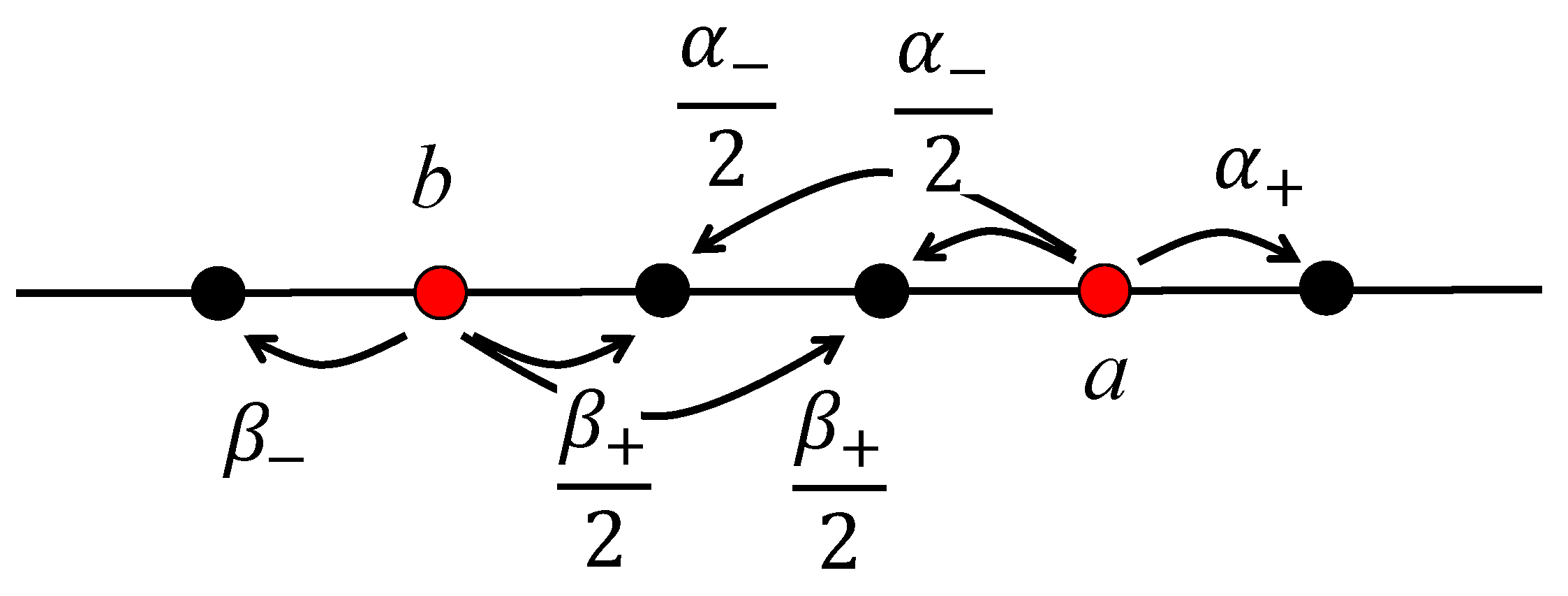
The Markov Model: A General View
3. The Markov Model: Closing the Spread Uniformly (Highly Competitive Regime)
3.1. Ergodicity and Invariant Measure for
3.2. Local Drift (LLN for the Prices)
3.3. Price Volatility (CLT for the Prices)
3.4. Large Deviations for the Spread
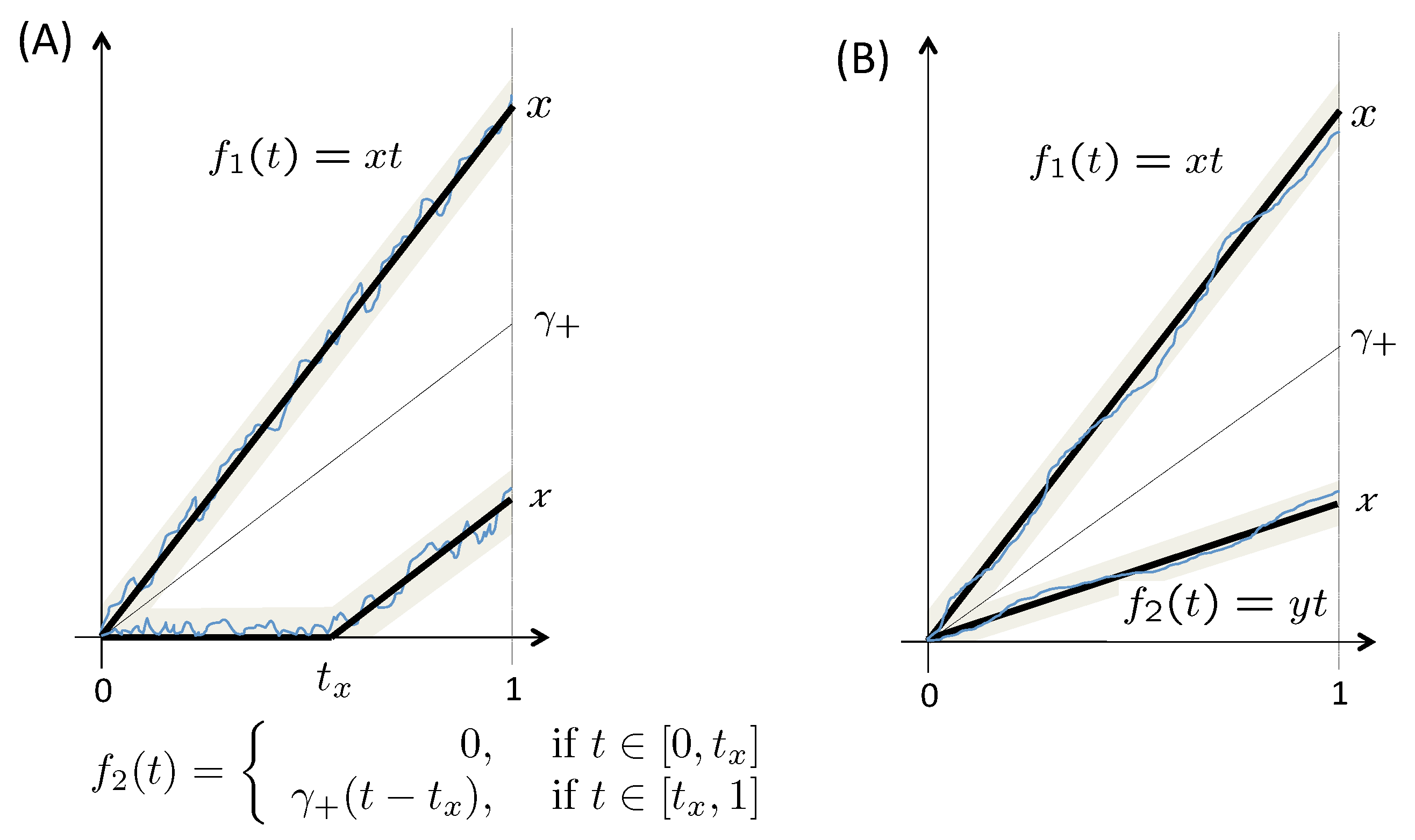
3.5. Large Deviations for the Prices
4. Numerical Simulations and Applications
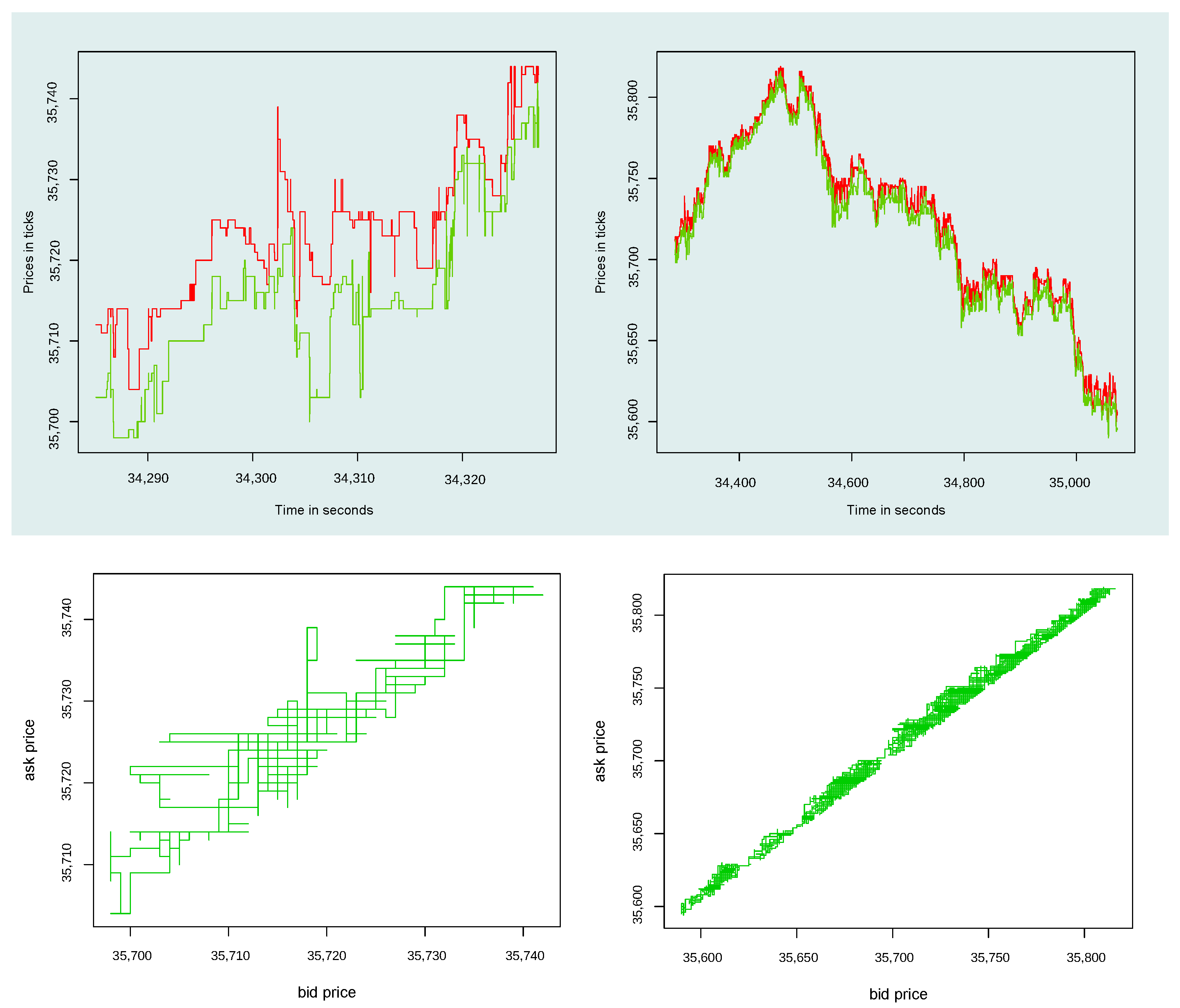
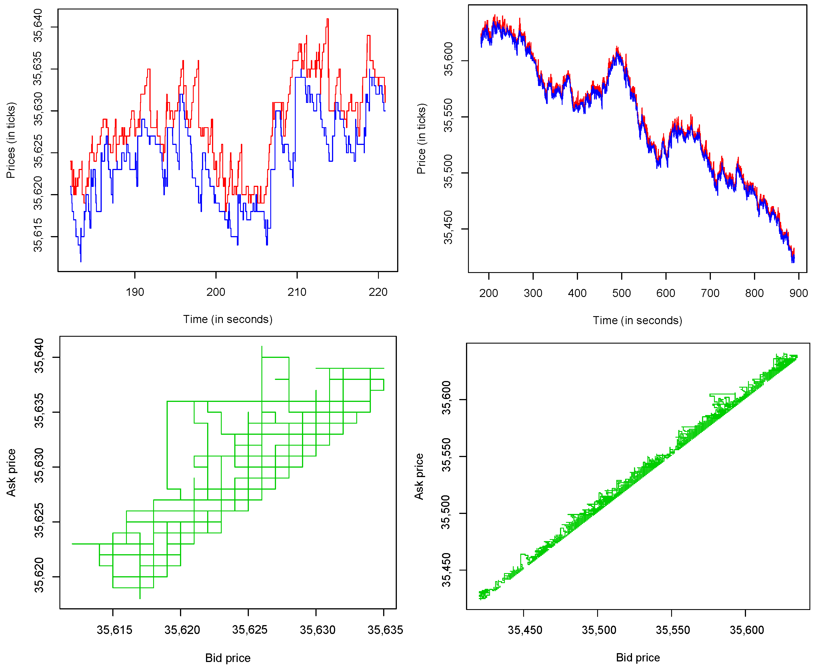
4.1. HFT Data
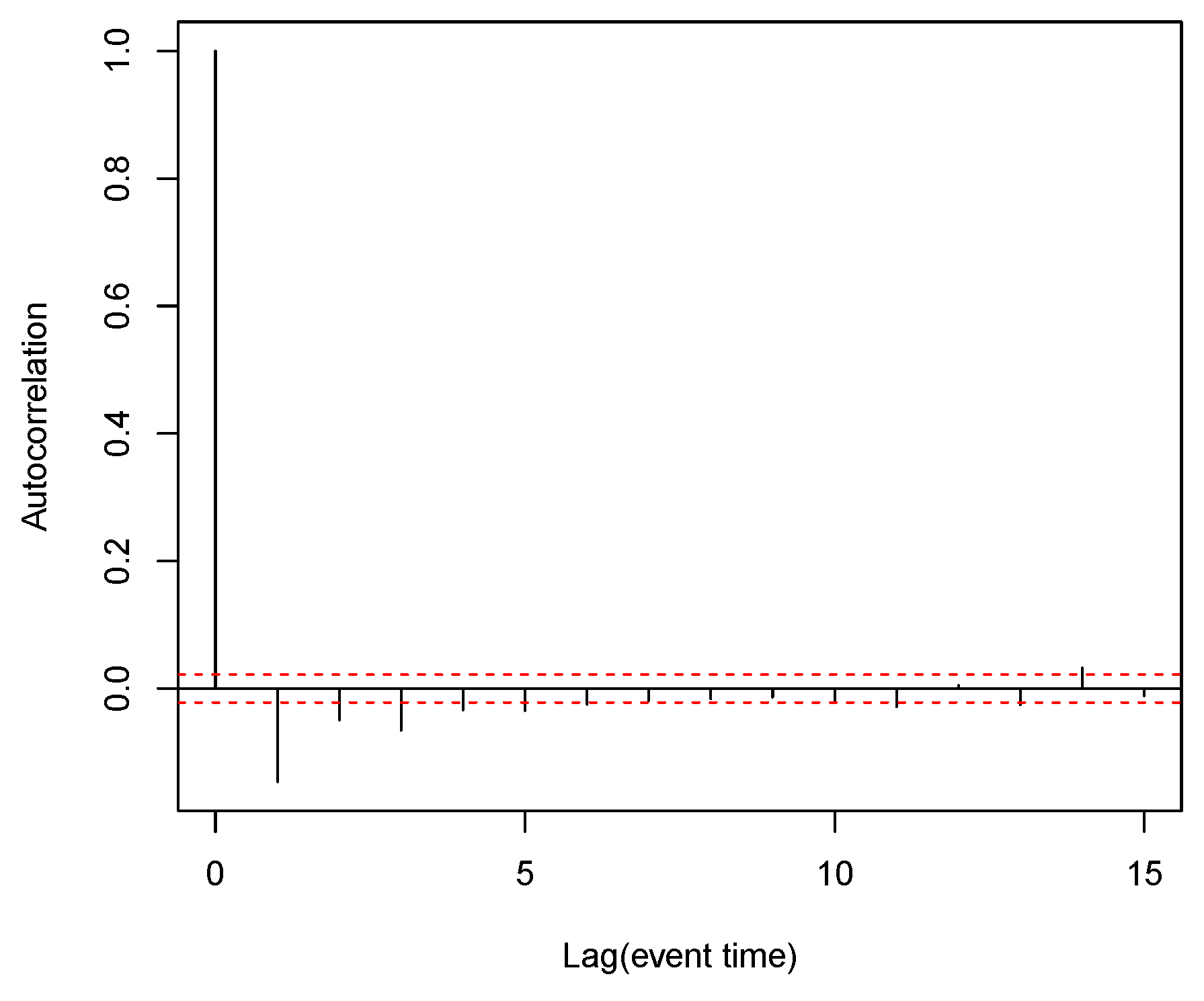
4.2. Empirical and Qualitative Facts
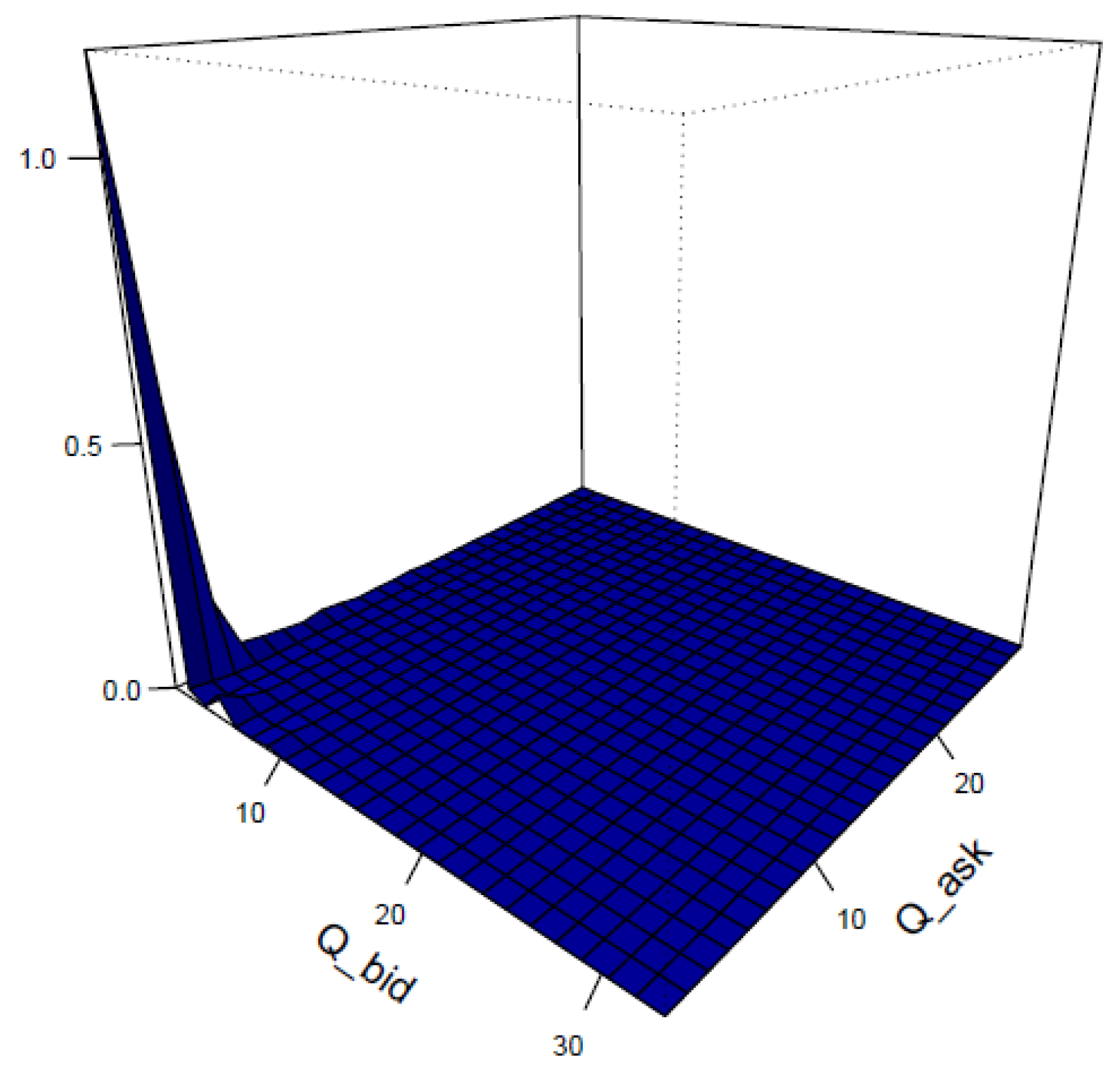
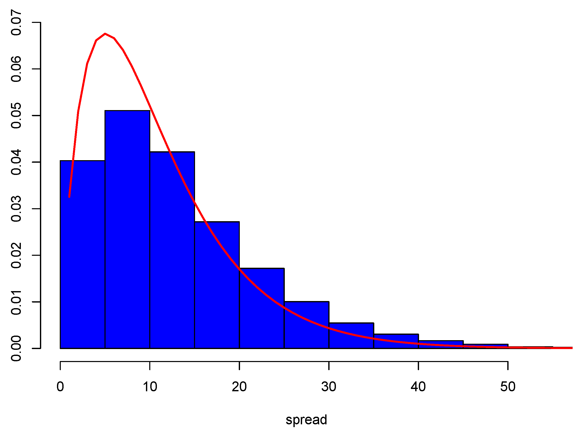
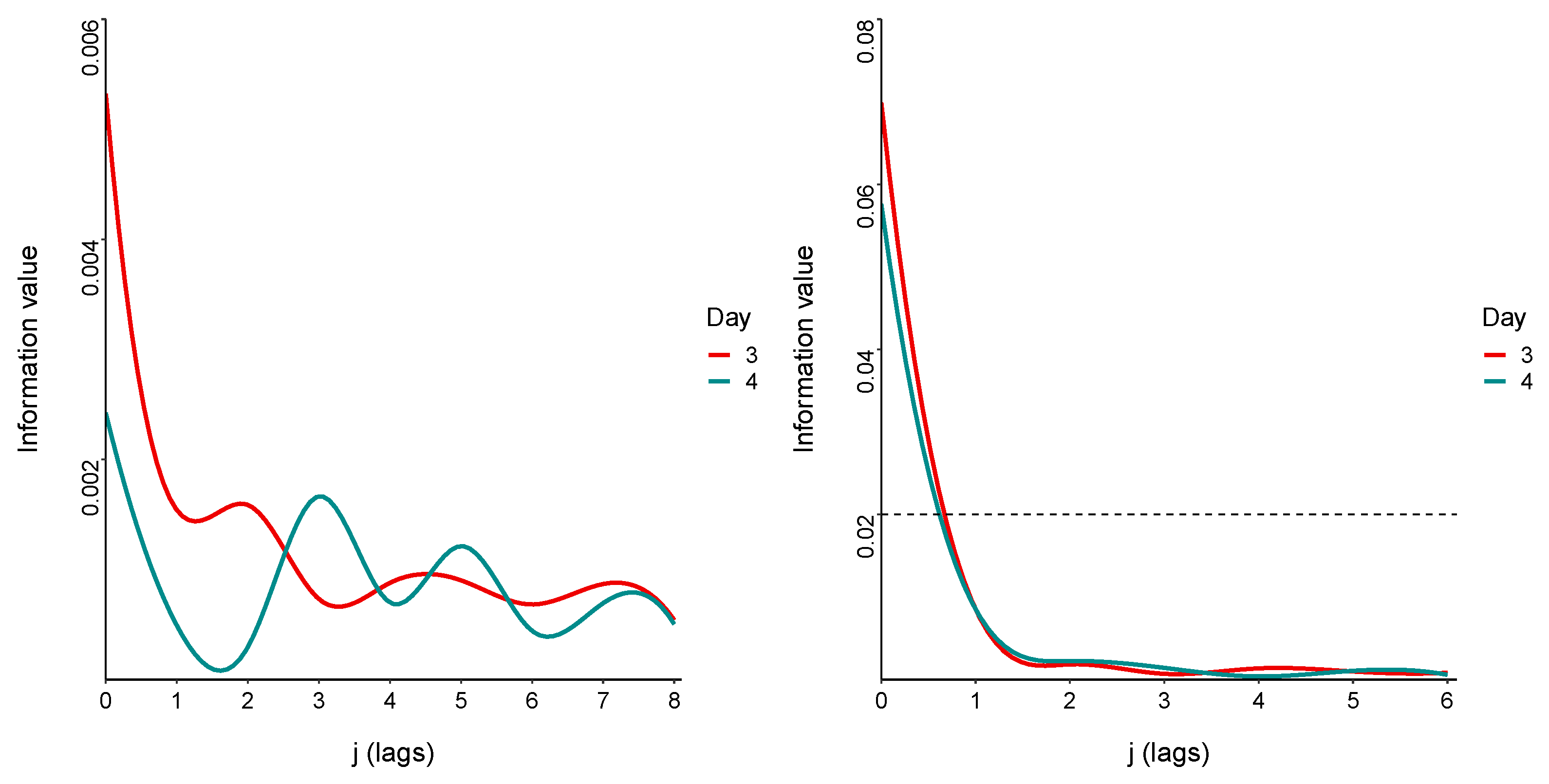
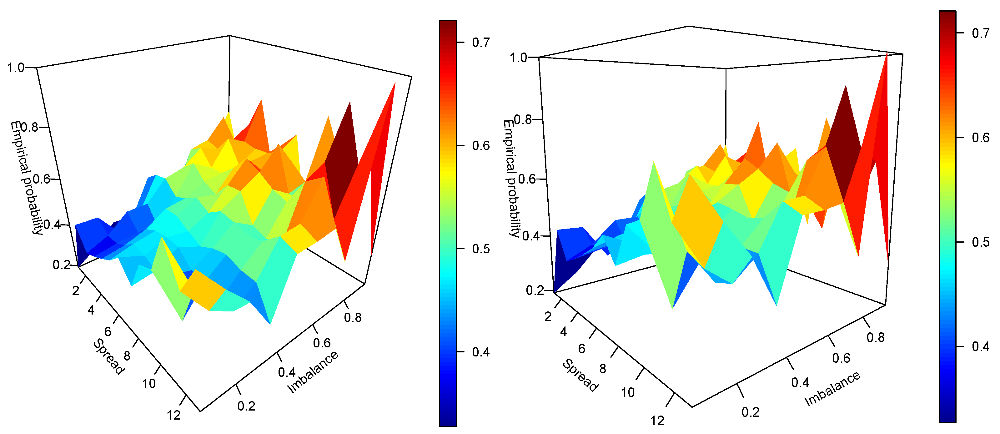
4.3. Parameter Estimation and Monte Carlo Experiments
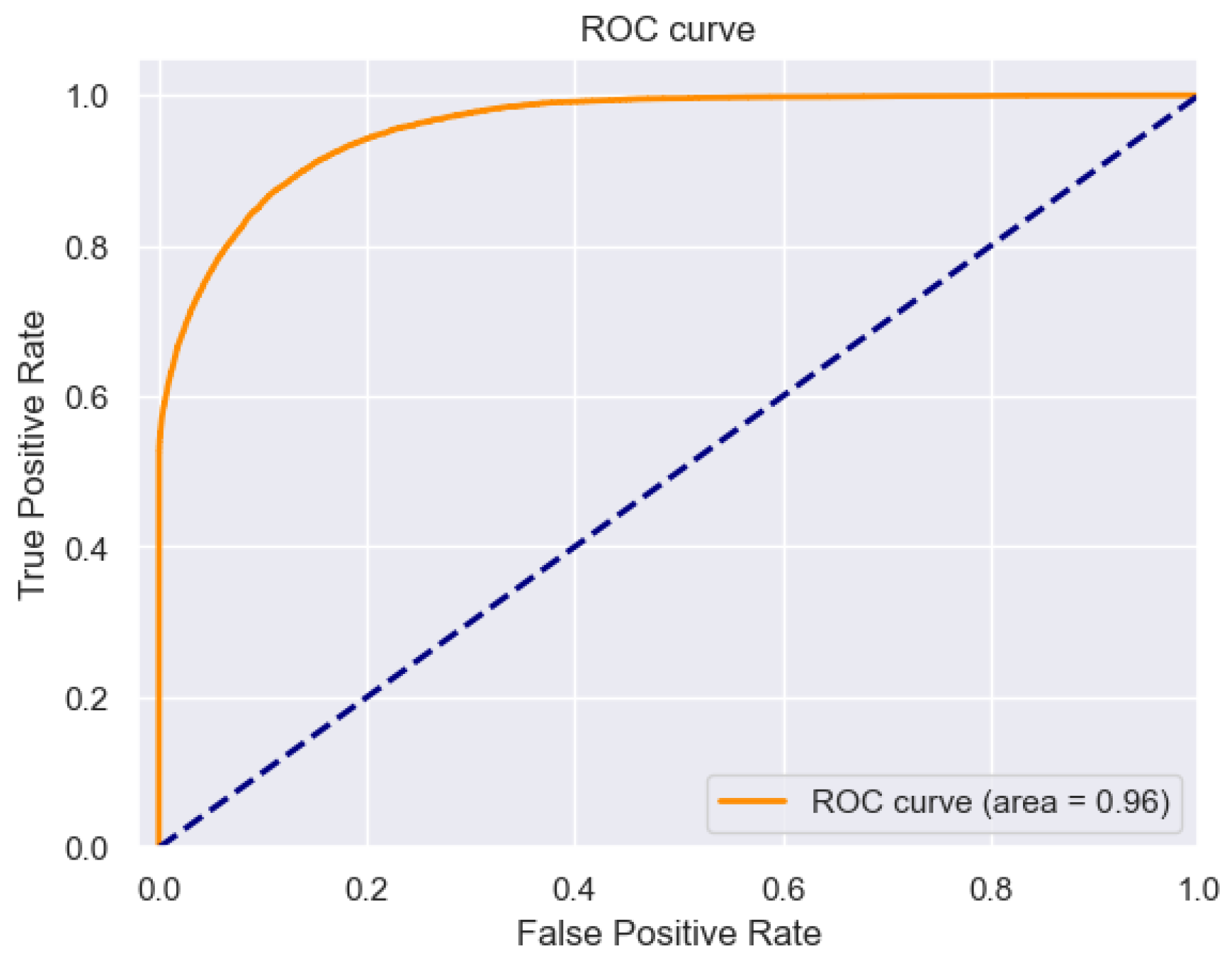
4.4. Application: Prediction of Next Price Jump Direction
5. Discussion: Other Regimes
5.1. Almost Uniform Catastrophes
5.2. Non-Competitive Regime
Model: Closing the Spread Polynomially
5.3. Low Liquidity with Gaps Regime
Model
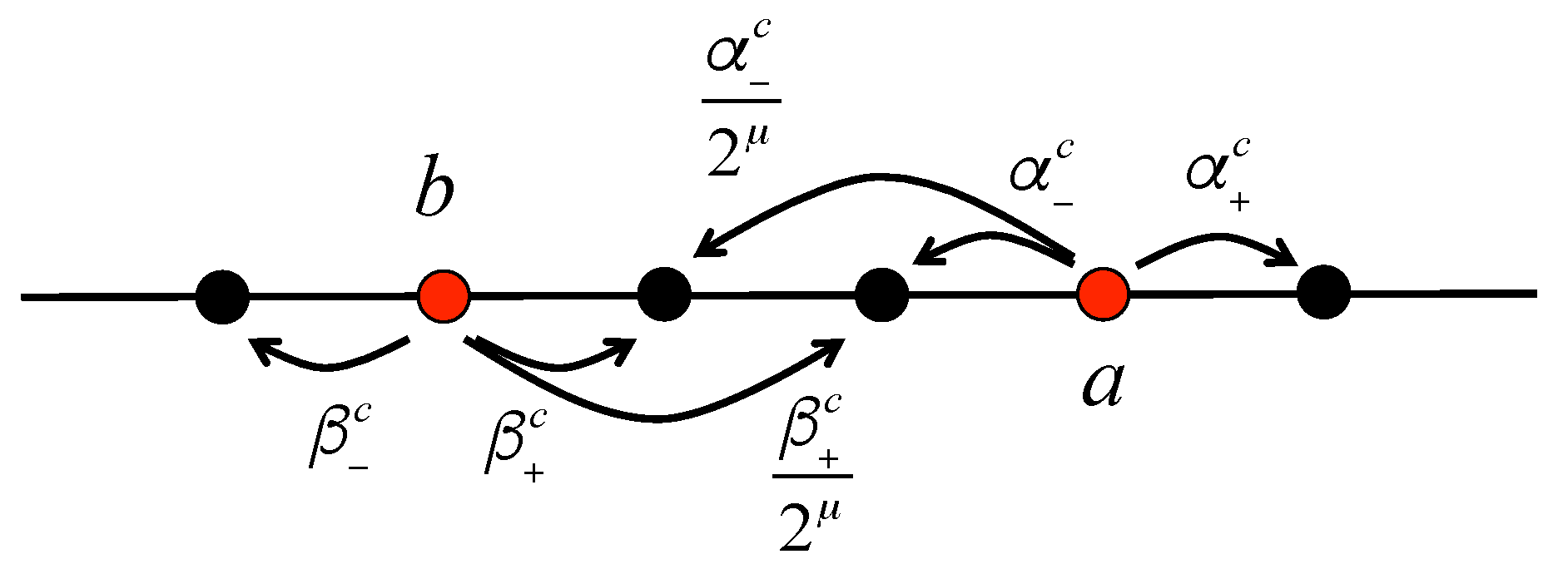
- with the rate , the chain decides to increase the ask price, and it chooses the increment according to the geometric distribution with parameter ;
- with the rate , the chain decides to decrease the ask price, and it chooses the increment according to the truncated geometric distribution with parameter and values ;
- with the rate , the chain decides to decrease the bid price, and it chooses the increment according to the geometric distribution with parameter ;
- with the rate , the chain decides to increase the bid price, and it chooses the increment according to the truncated geometric distribution with parameter and values .
6. Conclusions
Author Contributions
Funding
Data Availability Statement
Acknowledgments
Conflicts of Interest
Appendix A
Appendix A.1. Ergodicity and Invariant Measure for S(t): Proof of Theorem 1
Appendix A.2. Law of Large Numbers: Proof of Theorem 2
Appendix A.3. CLT for Embedding pn: Proof of Lemma 1
Appendix A.4. CLT for Continuous-Time P b (t): Proof of Theorem 3
References
- Biais, B.; Hillion, P.; Spatt, C. An empirical analysis of the limit order book and the order flow in the Paris Bourse. J. Financ. 1995, 50, 1655–1689. [Google Scholar] [CrossRef]
- Smith, E.; Farmer, J.D.; Gillemot, L.; Krishnamurthy, S. Statistical theory of the continuous double auction. Quant. Financ. 2003, 3, 481–514. [Google Scholar] [CrossRef]
- Bouchaud, J.P.; Farmer, J.D.; Lillo, F. How markets slowly digest changes in supply and demand. In Handbook of Financial Markets: Dynamics and Evolution; Elsevier: Amsterdam, The Netherlands, 2009; pp. 57–160. [Google Scholar]
- Cont, R.; Stoikov, S.; Talreja, R. A stochastic model for order book dynamics. Oper. Res. 2010, 58, 549–563. [Google Scholar] [CrossRef]
- Avellaneda, M.; Reed, J.; Stoikov, S. Forecasting prices from Level-I quotes in the presence of hidden liquidity. Algorithmic Financ. 2011, 1, 35–43. [Google Scholar] [CrossRef]
- Cont, R.; De Larrard, A. Price dynamics in a Markovian limit order market. SIAM J. Financ. Math. 2013, 4, 1–25. [Google Scholar] [CrossRef]
- Cont, R.; Mueller, M.S. A Stochastic Partial Differential Equation Model for Limit Order Book Dynamics. SIAM J. Financ. Math. 2019, 12, 744–787. [Google Scholar] [CrossRef]
- Golub, A.; Keane, J.; Poon, S.H. High frequency trading and mini flash crashes. arXiv 2012, arXiv:1211.6667. [Google Scholar] [CrossRef]
- Dall’Amico, L.; Fosset, A.; Bouchaud, J.P.; Benzaquen, M. How does latent liquidity get revealed in the limit order book? J. Stat. Mech. Theory Exp. 2019, 2019, 013404. [Google Scholar] [CrossRef]
- Lo, D.K.; Hall, A.D. Resiliency of the limit order book. J. Econ. Dyn. Control 2015, 61, 222–244. [Google Scholar] [CrossRef]
- Riccò, R.; Rindi, B.; Seppi, D.J. Information, Liquidity, and Dynamic Limit Order Markets; Bocconi University: Milano, Italy, 2022. [Google Scholar]
- Roll, R. A simple implicit measure of the effective bid-ask spread in an efficient market. J. Financ. 1984, 39, 1127–1139. [Google Scholar]
- Doyne Farmer, J.; Gillemot, L.; Lillo, F.; Mike, S.; Sen, A. What really causes large price changes? Quant. Financ. 2004, 4, 383–397. [Google Scholar] [CrossRef]
- Biais, B.; Weill, P.O. Liquidity Shocks and Order Book Dynamics; Technical Report; National Bureau of Economic Research: Cambridge, MA, USA, 2009. [Google Scholar]
- Logachov, A.; Logachova, O.; Yambartsev, A. The local principle of large deviations for compound Poisson process with catastrophes. Braz. J. Probab. Stat. 2021, 35, 205–223. [Google Scholar] [CrossRef]
- Logachov, A.; Logachova, O.; Yambartsev, A. Large deviations in a population dynamics with catastrophes. Stat. Probab. Lett. 2019, 149, 29–37. [Google Scholar] [CrossRef]
- Rojas, H.; Alvarez, C.; Rojas, N. Statistical Hypothesis Testing for Information Value (IV). arXiv 2023, arXiv:2309.13183. [Google Scholar]
- Menshikov, M.; Petritis, D. Explosion, implosion, and moments of passage times for continuous-time Markov chains: A semimartingale approach. Stoch. Process. Their Appl. 2014, 124, 2388–2414. [Google Scholar] [CrossRef]
- Jones, G.L. On the Markov chain central limit theorem. Probab. Surv. 2004, 1, 299–320. [Google Scholar] [CrossRef]
- Meyn, S.P.; Tweedie, R.L. Markov Chains and Stochastic Stability; Springer Science & Business Media: Berlin/Heidelberg, Germany, 2012. [Google Scholar]
- Popov, N. Geometric ergodicity conditions for countable Markov chains. Dokl. Akad. Nauk. Russ. Acad. Sci. 1977, 234, 316–319. [Google Scholar]


Disclaimer/Publisher’s Note: The statements, opinions and data contained in all publications are solely those of the individual author(s) and contributor(s) and not of MDPI and/or the editor(s). MDPI and/or the editor(s) disclaim responsibility for any injury to people or property resulting from any ideas, methods, instructions or products referred to in the content. |
© 2023 by the authors. Licensee MDPI, Basel, Switzerland. This article is an open access article distributed under the terms and conditions of the Creative Commons Attribution (CC BY) license (https://creativecommons.org/licenses/by/4.0/).
Share and Cite
Rojas, H.; Logachov, A.; Yambartsev, A. Order Book Dynamics with Liquidity Fluctuations: Asymptotic Analysis of Highly Competitive Regime. Mathematics 2023, 11, 4235. https://doi.org/10.3390/math11204235
Rojas H, Logachov A, Yambartsev A. Order Book Dynamics with Liquidity Fluctuations: Asymptotic Analysis of Highly Competitive Regime. Mathematics. 2023; 11(20):4235. https://doi.org/10.3390/math11204235
Chicago/Turabian StyleRojas, Helder, Artem Logachov, and Anatoly Yambartsev. 2023. "Order Book Dynamics with Liquidity Fluctuations: Asymptotic Analysis of Highly Competitive Regime" Mathematics 11, no. 20: 4235. https://doi.org/10.3390/math11204235
APA StyleRojas, H., Logachov, A., & Yambartsev, A. (2023). Order Book Dynamics with Liquidity Fluctuations: Asymptotic Analysis of Highly Competitive Regime. Mathematics, 11(20), 4235. https://doi.org/10.3390/math11204235