Global Asymptotic Stability and Synchronization of Fractional-Order Reaction–Diffusion Fuzzy BAM Neural Networks with Distributed Delays via Hybrid Feedback Controllers

Abstract

In this paper, the global asymptotic stability and global Mittag–Leffler stability of a class of fractional-order fuzzy bidirectional associative memory (BAM) neural networks with distributed delays is investigated. Necessary conditions are obtained by means of the Lyapunov functional method and inequality techniques. The hybrid feedback controllers are then developed to ensure the global asymptotic synchronization of these neural networks, resulting in two additional synchronization criteria. The derived conditions are applied to check the fractional-order fuzzy BAM neural network’s Mittag–Leffler stability and synchronization. Three examples are given to demonstrate the effectiveness of the achieved results.

1. Introduction

On the parallel perspective, neural networks having fractional-order derivatives generally possess boundless memory, which finds an advantage in comparison with common integer-order neural networks. In fact, the memory and heredity properties of certain materials and processes are known to be better represented by fractional-order derivatives [1,2]. Because of its wide range of applications in areas such as neural networks, quantum physics, optical systems, and optical image processing, fractional-order systems have been extensively investigated during the last several decades as a technique for precisely describing real systems [3,4,5,6,7,8,9,10,11].

In addition, there is a class of fuzzy cellular neural networks with delays that has been studied by numerous researchers using a variety of analytical and numerical methodologies. In comparison to normal cellular neural networks, a fuzzy cellular neural network uses fuzzy logic between its template input and/or output in addition to the sum of product operations. Hence, there has been a lot of research activity in the area of delayed fuzzy cellular neural networks [12,13,14], including recently studied fractional-order cases [15,16].

Bidirectional associative memory (BAM) neural networks with two layers of neuronal cells were first introduced by Kosko [17]. The neurons in the first layer are fully interconnected with the neurons in the second layer, but there is no interconnect between neurons in the same layer. Due to their application in numerous disciplines such as image and signal processing, pattern recognition, optimization, and autonomous control, BAM neural networks have received a lot of attention in the last decade [18,19]. As a result, the stability of BAM neural networks has been extensively studied, and many stability requirements for BAM neural networks have been published [20,21,22].

Global asymptotic stability is one of the most investigated stability behavior of real-world neural systems and artificial neural network systems. This is due to the fact that a globally asymptotically stable neural network system is promising for a fast convergence rate to a state of interest. The global asymptotic stability of an error neural network is closely related to the global asymptotic synchronization of the master and response systems. That is why global asymptotic stability and global asymptotic synchronization have received much attention among researchers [1,13,20,22]. Both notions are studied for integer-order as well as for fractional-order problems.

Podlubny and his coauthors proposed in [23] the Mittag–Leffler stability notion and the fractional Lyapunov direct approach to extend the use of fractional calculus in nonlinear systems, with the goal of improving both system theory and fractional calculus knowledge. Since then, the stability of Mittag–Leffler, generalized Mittag–Leffler stability, and synchronization have been examined for different classes of fractional-order neural networks [24,25,26,27], including BAM neural network models [28,29].

It is evident from the literature that most research work on delayed neural networks are devoted to simple cases of discrete delays. However, due to the presence of numerous parallel ways, neural networks usually exhibit a unique nature, resulting in a distribution of conduction velocities and propagation delays along these pathways. Due to the presence of a large number of parallel routes with different axon diameters and lengths, neural networks usually have a spatial extent. As a result, there will be a distribution of conduction velocities and propagation delays along these pathways. In these cases, signal transmission is not instantaneous and cannot be described using discrete delays; instead, continuously distributed and infinite delays are more appropriate [1,16,22,30,31,32,33].

When electrons move in asymmetric electromagnetic fields, diffusion effects cannot be avoided in the complex network models strictly speaking [2,12,34,35,36,37,38,39]. In signal transmission, the signal becomes weak due to diffusion, so it is very important to consider that the activation varies in space as well as in time, and the reaction–diffusion effects cannot be neglected in both biological and man-made networks [40]. The models covering time delay and reaction–diffusion are good mimicry for real neural networks in terms of application, but the existence of time delays and reaction–diffusion could bring about some undesirable behavior.

Motivated by the above considerations, we have studied the global asymptotic stability of fractional-order fuzzy BAM reaction–diffusion neural networks with discrete and distributed delays via hybrid feedback controllers. The main contributions of this research are:

1. The global asymptotic stability and synchronization of fractional-order fuzzy BAM neural networks with reaction–diffusion terms and mixed delays, including distributed ones, are investigated via hybrid feedback controllers.

2. By applying of stability theory for fractional models together with some inequality strategies, efficient criteria are obtained to guarantee the global Mittag–Leffler stability and synchronization.

3. We establish a uniform approach to dealing with discrete and distributed time delays under more general activation function assumptions.

4. The established conditions include the positive influence of reaction–diffusion terms on the stability and synchronization behavior and reduce the conservatism of the existing ones.

5. Finally, numerical examples are provided to demonstrate the correctness of the proposed results.

The rest of the paper is organized as follows. Some preliminary definitions and results related to fractional calculus are given in Section 2. The fractional-order fuzzy BAM neural network model, together with the controlled one are also introduced. Section 3 is devoted to our global asymptotic stability results. Global Mittag–Leffler synchronization criteria are established in Section 4. In Section 5, we elaborate some examples to demonstrate the validity and feasibility of the established results. Some conclusion notes and future directions of our research are discussed in Section 6.

2. Preliminaries and Problem Definition

In the present section, we first introduce some basic definitions and the corresponding results that are used later. Then, the fractional-order fuzzy BAM neural network model is formulated.

Definition 1

([41]). The Caputo fractional derivative of order β for a function $f\left(t\right)$ is defined by

$$\begin{array}{c}\hfill D^{\beta }f\left(\mathfrak{t}\right)=\frac{1}{\Gamma (n-\beta )}{\int }_b^{\mathfrak{t}}{(\mathfrak{t}-\tau )}^{n-\beta -1}{f}^{\left(n\right)}\left(\tau \right)d\tau ,\end{array}$$

in which $\mathfrak{t}\ge b$, $\mathfrak{t}\in \mathbb{R}$, $n-1<\beta <n\in \mathbb{N}$, and Γ is the standard Gamma function.

In this paper, we consider the following fractional-order reaction–diffusion fuzzy BAM neural network with mixed delays

$$\begin{array}{cc}\hfill \frac{{\partial }^{\lambda }{\zeta }_{\phi }\left(\mathfrak{t},\wp \right)}{\partial {\mathfrak{t}}^{\lambda }}& =\sum _{k=1}^q\frac{\partial }{\partial {\zeta }_k}(m_{\phi k}\frac{\partial {\zeta }_{\phi }\left(\mathfrak{t},\wp \right)}{\partial {\wp }_k})-d_{\phi }{\zeta }_{\phi }\left(\mathfrak{t},\wp \right)+\sum _{\varpi =1}^n{c}_{\phi \varpi }{f}_{\varpi }\left({\Im }_{\varpi }\left(\mathfrak{t},\wp \right)\right)\hfill \\ & +\sum _{\varpi =1}^n{a}_{\phi \varpi }{f}_{\varpi }\left({\Im }_{\varpi }(\mathfrak{t}-\tau ,\wp )\right)\hfill \\ & +\underset{\varpi =1}{\overset{n}{\bigwedge }}{u}_{\phi \varpi }{\int }_0^{\infty }{k}_{\phi \varpi }\left(s\right)f_{\varpi }\left({\Im }_{\varpi }(s-\tau ,\wp )\right)ds+\underset{\varpi =1}{\overset{n}{\bigwedge }}{P}_{\phi \varpi }{\Im }_{\varpi }\left(\mathfrak{t},\wp \right)\hfill \\ & +\underset{\varpi =1}{\overset{n}{\bigvee }}{v}_{\phi \varpi }{\int }_0^{\infty }{k}_{\phi \varpi }\left(s\right)f_{\varpi }\left({\Im }_{\varpi }(s-\tau ,\wp )\right)ds+\underset{\varpi =1}{\overset{n}{\bigvee }}{Q}_{\phi \varpi }{\Im }_{\varpi }\left(\mathfrak{t},\wp \right)+I_{\phi },\phi =1,2,\dots ,o,\hfill \\ \hfill \frac{{\partial }^{\lambda }{\Im }_{\varpi }\left(\mathfrak{t},\wp \right)}{\partial {\mathfrak{t}}^{\lambda }}& =\sum _{k=1}^q\frac{\partial }{\partial {\Im }_k}({\tilde{m}}_{\varpi k}\frac{\partial {\Im }_{\varpi }\left(t,\wp \right)}{\partial {\wp }_k})-{\tilde{d}}_{\varpi }{\Im }_{\varpi }\left(\mathfrak{t},\wp \right)+\sum _{\phi =1}^o{\tilde{c}}_{\varpi \phi }{g}_{\phi }\left({\zeta }_{\phi }(\mathfrak{t},\wp )\right)\hfill \\ & +\sum _{\phi =1}^o{\tilde{a}}_{\varpi \phi }{g}_{\phi }\left({\zeta }_{\phi }(\mathfrak{t}-\tau ,\wp )\right)\hfill \\ & +\underset{\phi =1}{\overset{o}{\bigwedge }}{\tilde{u}}_{\varpi \phi }{\int }_0^{\infty }{k}_{\varpi \phi }\left(s\right)g_{\phi }\left({\zeta }_{\varpi }(s-\tau ,\wp )\right)ds+\underset{\phi =1}{\overset{o}{\bigwedge }}{\tilde{P}}_{\varpi \phi }{\zeta }_{\phi }(\mathfrak{t},\wp )\hfill \\ & +\underset{\phi =1}{\overset{o}{\bigvee }}{\tilde{v}}_{\varpi \phi }{\int }_0^{\infty }{k}_{\varpi \phi }\left(s\right)g_{\phi }\left({\zeta }_{\phi }(s-\tau ,\wp )\right)ds+\underset{\phi =1}{\overset{o}{\bigvee }}{\tilde{Q}}_{\varpi \phi }{\zeta }_{\phi }(\mathfrak{t},\wp )+J_{\varpi },\varpi =1,2,\dots ,n,\hfill \end{array}$$

(1)

where n and o denote the number of neurons in the ℑ-layer and $\zeta$-layer, respectively. For $\phi =1,2,\dots ..,o$, $\varpi =1,2,\dots .,n,$ and $\wp ={({\wp }_1,{\wp }_2,\dots ,{\wp }_q)}^T\in \Omega \subset R^q$, $\Omega$ is a bounded compact set with a smooth boundary $\partial \Omega$, and mess$(\Omega )>0$ in the space $R^q$; ${\zeta }_{\phi }(\mathfrak{t},\wp )$ and ${\Im }_{\varpi }(\mathfrak{t},\wp )$ are the states of the $\phi$th neuron and the $\varpi$th neurons at time t and space ℘, respectively; $d_{\phi }$ and ${\tilde{d}}_{\varpi }$ indicate the rates with which the $\phi$th neuron and $\varpi$th neuron will reset their potentials to the resting states in isolation when disconnecting the network and external inputs; $c_{\phi \varpi }$, $a_{\phi \varpi }$, ${\tilde{c}}_{\varpi \phi }$, and ${\tilde{a}}_{\varpi \phi }$ are elements of the fuzzy feedback MIN template and fuzzy feedback MAX template, fuzzy feed-forward MIN template and fuzzy feed-forward MAX template, respectively; $\tau$ is the discrete transmission delay; $\bigwedge$ and $\bigvee$ denote the fuzzy AND and fuzzy OR operations, respectively; $I_{\phi }$ and $J_{\varpi }$ denote the external inputs on the $\phi$th neurons in the ℑ-layer and the $\varpi$th neurons in the $\zeta$-layer, respectively. The smooth functions $m_{\phi k}\ge 0$ and ${\tilde{m}}_{\varpi k}\ge 0$ correspond to the transmission diffusion operators along the $\phi$th neurons and the $\varpi$th neurons, respectively, $u_{\phi \varpi }$, $v_{\varpi \phi }$, $P_{\varpi \phi }$, and $Q_{\varpi \phi }$ are elements of the fuzzy feedback MIN template and fuzzy feedback MAX template in the ℑ-layer, respectively. ${\tilde{u}}_{\phi \varpi }$, ${\tilde{v}}_{\varpi \phi }$, ${\tilde{P}}_{\phi \varpi }$, and ${\tilde{Q}}_{\phi \varpi }$ are elements of the fuzzy feedback MIN template and fuzzy feedback MAX template in the $\zeta$-layer. $k_{\phi \varpi }(·)$ and $k_{\varpi \phi }(·)$ are delay kernels functions. $f_{\varpi }(·)$ and $g_{\phi }(·)$ are signal transmission functions of $\varpi$th neurons and $\phi$th neurons, respectively, and

$$\frac{{\partial }^{\lambda }p\left(\mathfrak{t},\wp \right)}{\partial {\mathfrak{t}}^{\lambda }}=\frac{1}{\Gamma (1-\lambda )}{\int }_0^t\frac{\partial p\left(s,\wp \right)}{\partial s}\frac{ds}{{(\mathfrak{t}-s)}^{\lambda }},t>0,0<\lambda <1$$

for a function $p\in C^1[[0,b]\times \Omega ,\mathbb{R}]$, $b>0$ [7].

The corresponding response system with feedback controllers ${\mathcal{U}}_{\phi }(\mathfrak{t},\wp )$ and ${\mathcal{U}}_{\varpi }(\mathfrak{t},\wp )$ is described by

$$\begin{array}{cc}\hfill \frac{{\partial }^{\lambda }{\overline{\zeta }}_{\phi }\left(\mathfrak{t},\wp \right)}{\partial {\mathfrak{t}}^{\lambda }}& =\sum _{k=1}^q\frac{\partial }{\partial {\wp }_k}(m_{\phi k}\frac{\partial {\overline{\zeta }}_{\phi }\left(\mathfrak{t},\wp \right)}{\partial {\wp }_k})-d_{\phi }{\overline{\zeta }}_{\phi }\left(\mathfrak{t},\wp \right)+\sum _{\varpi =1}^n{c}_{\phi \varpi }{f}_{\varpi }\left({\overline{\Im }}_{\varpi }\left(\mathfrak{t},\wp \right)\right)\hfill \\ & +\sum _{\varpi =1}^n{a}_{\phi \varpi }{f}_{\varpi }\left({\overline{\Im }}_{\varpi }(\mathfrak{t}-\tau ,\wp )\right)+\underset{\varpi =1}{\overset{n}{\bigwedge }}{u}_{\phi \varpi }{\int }_0^{\infty }{k}_{\phi \varpi }\left(s\right)f_{\varpi }\left({\overline{\Im }}_{\varpi }(s-\tau ,\wp )\right)ds\hfill \\ & +\underset{\varpi =1}{\overset{n}{\bigwedge }}{P}_{\phi \varpi }{\overline{\Im }}_{\varpi }(\mathfrak{t},\wp )+\underset{\varpi =1}{\overset{n}{\bigvee }}{v}_{\phi \varpi }{\int }_0^{\infty }{k}_{\phi \varpi }\left(s\right)f_{\varpi }\left({\overline{\Im }}_{\varpi }(s-\tau ,\wp )\right)ds\hfill \\ & +\underset{\varpi =1}{\overset{n}{\bigvee }}{Q}_{\phi \varpi }{\overline{\Im }}_{\varpi }(t,\wp )+I_{\phi }+{\mathcal{U}}_{\phi }(\mathfrak{t},\wp ),\phi =1,2,\dots ,o,\hfill \\ \hfill \frac{{\partial }^{\lambda }{\overline{\Im }}_{\varpi }\left(\mathfrak{t},\wp \right)}{\partial {\mathfrak{t}}^{\lambda }}& =\sum _{k=1}^q\frac{\partial }{\partial {\wp }_k}({\tilde{m}}_{\varpi k}\frac{\partial {\overline{\Im }}_{\varpi }\left(\mathfrak{t},\wp \right)}{\partial {\wp }_k})-{\tilde{d}}_{\varpi }{\overline{\Im }}_{\varpi }\left(\mathfrak{t},\wp \right)+\sum _{\phi =1}^o{\tilde{c}}_{\varpi \phi }{g}_{\phi }\left({\overline{\zeta }}_{\phi }(\mathfrak{t},\wp )\right)\hfill \\ & +\sum _{\phi =1}^o{\tilde{a}}_{\varpi \phi }{g}_{\phi }\left({\overline{\zeta }}_{\phi }(\mathfrak{t}-\tau ,\wp )\right)+\underset{\phi =1}{\overset{o}{\bigwedge }}{\tilde{u}}_{\varpi \phi }{\int }_0^{\infty }{k}_{\varpi \phi }\left(s\right)g_{\phi }\left({\overline{\zeta }}_{\phi }(s-\tau ,\wp )\right)ds\hfill \\ & +\underset{\phi =1}{\overset{o}{\bigwedge }}{\tilde{P}}_{\varpi \phi }{\overline{\zeta }}_{\phi }(t,\wp )+\underset{\phi =1}{\overset{o}{\bigvee }}{\tilde{v}}_{\varpi \phi }{\int }_0^{\infty }{k}_{\varpi \phi }\left(s\right)g_{\phi }\left({\overline{\zeta }}_{\phi }(s-\tau ,\wp )\right)ds\hfill \\ & +\underset{\phi =1}{\overset{o}{\bigvee }}{\tilde{Q}}_{\varpi \phi }{\overline{\zeta }}_{\phi }(\mathfrak{t},\wp )+J_{\varpi }+{\mathcal{U}}_{\varpi }(\mathfrak{t},\wp ),\varpi =1,2,\dots ,n.\hfill \end{array}$$

(2)

For ${\xi }_{\phi }(\mathfrak{t},\wp )={\overline{\zeta }}_{\phi }(\mathfrak{t},\wp )-{\zeta }_{\phi }(\mathfrak{t},\wp )$ and ${\overline{\xi }}_{\varpi }(\mathfrak{t},\wp )={\overline{\Im }}_{\varpi }(\mathfrak{t},\wp )-{\Im }_{\varpi }(\mathfrak{t},\wp )$, the error system is defined by

$$\begin{array}{cc}\hfill \frac{{\partial }^{\lambda }{\xi }_{\phi }\left(\mathfrak{t},\wp \right)}{\partial {\mathfrak{t}}^{\lambda }}& =\sum _{k=1}^q\frac{\partial }{\partial {\wp }_k}(m_{\phi k}\frac{\partial {\xi }_{\phi }\left(t,\wp \right)}{\partial {\wp }_k})-d_{\phi }{\xi }_{\phi }\left(\mathfrak{t},\wp \right)\hfill \\ & +\left[\sum _{\varpi =1}^n{c}_{\phi \varpi }{f}_{\varpi }\left({\overline{\Im }}_{\varpi }\left(\mathfrak{t},\wp \right)\right)-\sum _{\varpi =1}^n{c}_{\phi \varpi }{f}_{\varpi }\left({\Im }_{\varpi }\left(\mathfrak{t},\wp \right)\right)\right]\hfill \\ & +\left[\sum _{\varpi =1}^n{a}_{\phi \varpi }{f}_{\varpi }\left({\overline{\Im }}_{\varpi }(\mathfrak{t}-\tau ,\wp )\right)-\sum _{\varpi =1}^n{a}_{\phi \varpi }{f}_{\varpi }\left({\Im }_{\varpi }(\mathfrak{t}-\tau ,\wp )\right)\right]\hfill \\ & +\left[\underset{\varpi =1}{\overset{n}{\bigwedge }}{u}_{\phi \varpi }{\int }_0^{\infty }{k}_{\phi \varpi }\left(s\right)f_{\varpi }\left({\overline{\Im }}_{\varpi }(s-\tau ,\wp )\right)ds-\underset{\varpi =1}{\overset{n}{\bigwedge }}{u}_{\phi \varpi }{\int }_0^{\infty }{k}_{\phi \varpi }\left(s\right)f_{\varpi }\left({\Im }_{\varpi }(s-\tau ,\wp )\right)ds\right]\hfill \\ & +[\underset{\varpi =1}{\overset{n}{\bigvee }}{v}_{\phi \varpi }{\int }_0^{\infty }{k}_{\phi \varpi }\left(s\right)f_{\varpi }\left({\overline{\Im }}_{\varpi }(s-\tau ,\wp )\right)ds-\underset{\varpi =1}{\overset{n}{\bigvee }}{v}_{\phi \varpi }{\int }_0^{\infty }{k}_{\phi \varpi }\left(s\right)f_{\varpi }\left({\Im }_{\varpi }(s-\tau ,\wp )\right)ds]\hfill \\ & +{\mathcal{U}}_{\phi }(\mathfrak{t},\wp ),\phi =1,2,\dots ,o,\hfill \end{array}$$

$$\begin{array}{cc}\hfill \frac{{\partial }^{\lambda }{\overline{\xi }}_{\varpi }\left(\mathfrak{t},\wp \right)}{\partial {\mathfrak{t}}^{\lambda }}& =\sum _{k=1}^q\frac{\partial }{\partial {\wp }_k}({\tilde{m}}_{\varpi k}\frac{\partial {\overline{\xi }}_{\varpi }\left(t,\wp \right)}{\partial {\wp }_k})-{\tilde{d}}_{\varpi }{\overline{\xi }}_{\varpi }\left(t,\wp \right)\hfill \\ & +\left[\sum _{\phi =1}^o{\tilde{c}}_{\varpi \phi }{g}_{\phi }\left({\overline{\zeta }}_{\phi }(t,\wp )\right)-\sum _{\phi =1}^o{\tilde{c}}_{\varpi \phi }{g}_{\phi }\left({\zeta }_{\phi }(\mathfrak{t},\wp )\right)\right]\hfill \\ & +\left[\sum _{\phi =1}^o{\tilde{a}}_{\varpi \phi }{g}_{\phi }\left({\overline{\zeta }}_{\phi }(\mathfrak{t}-\tau ,\wp )\right)-\sum _{\phi =1}^o{\tilde{a}}_{\varpi \phi }{g}_{\phi }\left({\zeta }_{\phi }(t-\tau ,\wp )\right)\right]\hfill \\ & +\left[\underset{\phi =1}{\overset{o}{\bigwedge }}{\tilde{u}}_{\varpi \phi }{\int }_0^{\infty }{k}_{\varpi \phi }\left(s\right)g_{\phi }\left({\overline{\zeta }}_{\phi }(s-\tau ,\wp )\right)ds-\underset{\phi =1}{\overset{o}{\bigwedge }}{\tilde{u}}_{\varpi \phi }{\int }_0^{\infty }{k}_{\varpi \phi }\left(s\right)g_{\phi }\left({\zeta }_{\phi }(s-\tau ,\wp )\right)ds\right]\hfill \\ & +\left[\underset{\phi =1}{\overset{o}{\bigvee }}{\tilde{v}}_{\varpi \phi }{\int }_0^{\infty }{k}_{\varpi \phi }\left(s\right)g_{\phi }\left({\overline{\zeta }}_{\phi }(s-\tau ,\wp )\right)ds-\underset{\phi =1}{\overset{o}{\bigvee }}{\tilde{v}}_{\varpi \phi }{\int }_0^{\infty }{k}_{\varpi \phi }\left(s\right)g_{\phi }\left({\zeta }_{\phi }(s-\tau ,\wp )\right)ds\right]\hfill \\ & +{\mathcal{U}}_{\varpi }(\mathfrak{t},\wp ),\varpi =1,2,\dots ,n.\hfill \end{array}$$

(3)

We design a suitable controller for the error system (3). Let ${\mathcal{U}}_{\phi }(\mathfrak{t},\wp )={\mathcal{U}}_{1\phi }(\mathfrak{t},\wp )+{\mathcal{U}}_{2\phi }(\mathfrak{t},\wp )$, where ${\mathcal{U}}_{1\phi }(\mathfrak{t},\wp )=-{\mathfrak{t}}_{\phi }{\xi }_{\phi }(\mathfrak{t},\wp )$ and ${\mathcal{U}}_{2\phi }(\mathfrak{t},\wp )=-{\Psi }_{\phi }{\xi }_{\phi }(\mathfrak{t},\wp )$ and ${\mathcal{U}}_{\varpi }(\mathfrak{t},\wp )$$={\mathcal{U}}_{1\varpi }(\mathfrak{t},\wp )+{\mathcal{U}}_{2\varpi }(\mathfrak{t},\wp )$, where ${\mathcal{U}}_{1\varpi }(\mathfrak{t},\wp )=-{\varpi }_{\varpi }{\overline{\xi }}_{\varpi }(\mathfrak{t},\wp )$ and ${\mathcal{U}}_{2\varpi }(\mathfrak{t},\wp )=-{\varrho }_{\varpi }{\overline{\xi }}_{\varpi }(\mathfrak{t},\wp )$, where ${\mathfrak{t}}_{\phi },{\Psi }_{\phi },{\varpi }_{\varpi },$ and ${\varrho }_{\varpi }$ are positive constants. Then, system (3) has the form

$$\begin{array}{cc}\hfill \frac{{\partial }^{\lambda }{\xi }_{\phi }\left(\mathfrak{t},\wp \right)}{\partial {\mathfrak{t}}^{\lambda }}& =\sum _{k=1}^q\frac{\partial }{\partial {\wp }_k}(m_{\phi k}\frac{\partial {\xi }_{\phi }\left(\mathfrak{t},\wp \right)}{\partial {\wp }_k})-d_{\phi }{\xi }_{\phi }\left(\mathfrak{t},\wp \right)\hfill \\ & +\left[\sum _{\varpi =1}^n{c}_{\phi \varpi }{f}_{\varpi }\left({\overline{\Im }}_{\varpi }\left(\mathfrak{t},\wp \right)\right)-\sum _{\varpi =1}^n{c}_{\phi \varpi }{f}_{\varpi }\left({\Im }_{\varpi }\left(\mathfrak{t},\wp \right)\right)\right]\hfill \\ & +\left[\sum _{\varpi =1}^n{a}_{\phi \varpi }{f}_{\varpi }\left({\overline{\Im }}_{\varpi }(\mathfrak{t}-\tau ,\wp )\right)-\sum _{\varpi =1}^n{a}_{\phi \varpi }{f}_{\varpi }\left({\Im }_{\varpi }(t-\tau ,\wp )\right)\right]\hfill \\ & +\left[\underset{\varpi =1}{\overset{n}{\bigwedge }}{u}_{\phi \varpi }{\int }_0^{\infty }{k}_{\phi \varpi }\left(s\right)f_{\varpi }\left({\overline{\Im }}_{\varpi }(s-\tau ,\wp )\right)ds-\underset{\varpi =1}{\overset{n}{\bigwedge }}{u}_{\phi \varpi }{\int }_0^{\infty }{k}_{\phi \varpi }\left(s\right)f_{\varpi }\left({\Im }_{\varpi }(s-\tau ,\wp )\right)ds\right]\hfill \\ & +\left[\underset{\varpi =1}{\overset{n}{\bigvee }}{v}_{\phi \varpi }{\int }_0^{\infty }{k}_{\phi \varpi }\left(s\right)f_{\varpi }\left({\overline{\Im }}_{\varpi }(s-\tau ,\wp )\right)ds-\underset{\varpi =1}{\overset{n}{\bigvee }}{v}_{\phi \varpi }{\int }_0^{\infty }{k}_{\phi \varpi }\left(s\right)f_{\varpi }\left({\Im }_{\varpi }(s-\tau ,\wp )\right)ds\right]\hfill \\ & -{\mathfrak{t}}_{\phi }{\xi }_{\phi }(t,\wp )-{\Psi }_{\phi }{\xi }_{\phi }(t,\wp ),\phi =1,2,\dots ,o,\hfill \end{array}$$

$$\begin{array}{cc}\hfill \frac{{\partial }^{\lambda }{\overline{\xi }}_{\varpi }\left(\mathfrak{t},\wp \right)}{\partial {\mathfrak{t}}^{\lambda }}& =\sum _{k=1}^q\frac{\partial }{\partial {\wp }_k}({\tilde{m}}_{\varpi k}\frac{\partial {\overline{\xi }}_{\varpi }\left(\mathfrak{t},\wp \right)}{\partial {\wp }_k})-{\tilde{d}}_{\varpi }{\overline{\xi }}_{\varpi }\left(\mathfrak{t},\wp \right)\hfill \\ & +\left[\sum _{\phi =1}^o{\tilde{c}}_{\varpi \phi }{g}_{\phi }\left({\overline{\zeta }}_{\phi }(t,\wp )\right)-\sum _{\phi =1}^o{\tilde{c}}_{\varpi \phi }{g}_{\phi }\left({\zeta }_{\phi }(t,\wp )\right)\right]\hfill \\ & +\left[\sum _{\phi =1}^o{\tilde{a}}_{\varpi \phi }{g}_{\phi }\left({\overline{\zeta }}_{\phi }(\mathfrak{t}-\tau ,\wp )\right)-\sum _{\phi =1}^o{\tilde{a}}_{\varpi \phi }{g}_{\phi }\left({\zeta }_{\phi }(\mathfrak{t}-\tau ,\wp )\right)\right]\hfill \\ & +\left[\underset{\phi =1}{\overset{o}{\bigwedge }}{\tilde{u}}_{\varpi \phi }{\int }_0^{\infty }{k}_{\varpi \phi }\left(s\right)g_{\phi }\left({\overline{\zeta }}_{\phi }(s-\tau ,\wp )\right)ds-\underset{\phi =1}{\overset{o}{\bigwedge }}{\tilde{u}}_{\varpi \phi }{\int }_0^{\infty }{k}_{\varpi \phi }\left(s\right)g_{\phi }\left({\zeta }_{\phi }(s-\tau ,\wp )\right)ds\right]\hfill \\ & +\left[\underset{\phi =1}{\overset{o}{\bigvee }}{\tilde{v}}_{\varpi \phi }{\int }_0^{\infty }{k}_{\varpi \phi }\left(s\right)g_{\phi }\left({\overline{\zeta }}_{\phi }(s-\tau ,\wp )\right)ds-\underset{\phi =1}{\overset{o}{\bigvee }}{\tilde{v}}_{\varpi \phi }{\int }_0^{\infty }{k}_{\varpi \phi }\left(s\right)g_{\phi }\left({\zeta }_{\phi }(s-\tau ,\wp )\right)ds\right]\hfill \\ & -{\varpi }_{\varpi }{\overline{\xi }}_{\varpi }(\mathfrak{t},\wp )-{\varrho }_{\varpi }{\overline{\xi }}_{\varpi }(\mathfrak{t},\wp ),\varpi =1,2,\dots ,n.\hfill \end{array}$$

(4)

We investigate the error system (4) under the following initial and boundary conditions:

$$\begin{array}{cc}\hfill {\xi }_{\phi }\left(\mathfrak{s},\wp \right)& ={\varphi }_{\phi }\left(\mathfrak{s},\wp \right),\mathfrak{s}\in (-\infty ,0],\wp \in \Omega ,\hfill \\ \hfill {\overline{\xi }}_{\varpi }\left(\mathfrak{s},\wp \right)& ={\tilde{\varphi }}_{\varpi }\left(\mathfrak{s},\wp \right),\mathfrak{s}\in (-\infty ,0],\wp \in \Omega ,\hfill \\ \hfill {\xi }_{\phi }\left(\mathfrak{t},\wp \right)& =0,\mathfrak{t}\in \mathbb{R},\wp \in \partial \Omega ,\hfill \\ \hfill {\overline{\xi }}_{\varpi }\left(\mathfrak{t},\wp \right)& =0,\mathfrak{t}\in \mathbb{R},\wp \in \partial \Omega ,\phi =1,2,\dots ,o,\varpi =1,2,\dots ,n,\hfill \end{array}$$

(5)

where ${\varphi }_{\phi }$ and ${\tilde{\varphi }}_{\varpi }$ are continuous initial functions.

In our stability analysis, we need the following assumptions.

Assumption 1.

For ${\vartheta }_{\varpi },{\overline{\vartheta }}_{\varpi }\in \mathbb{R}$ and ${\zeta }_{\phi },{\overline{\zeta }}_{\phi }\in \mathbb{R}$, the activation functions $f_{\varpi }$ and $g_{\phi }$ satisfy

$$\begin{array}{c}\hfill \left|\underset{\varpi =1}{\overset{n}{\bigwedge }}{u}_{\phi \varpi }{f}_{\varpi }\left({\vartheta }_{\varpi }\right)-\underset{\varpi =1}{\overset{n}{\bigwedge }}{u}_{\phi \varpi }{f}_{\varpi }\left({\overline{\vartheta }}_{\varpi }\right)\right|\le \sum _{\varpi =1}^n|u_{\phi \varpi }|\left|f_{\varpi }\left({\vartheta }_{\varpi }\right)-f_{\varpi }\left({\overline{\vartheta }}_{\varpi }\right)\right|,\varpi =1,2,\dots ,n,\\ \hfill \left|\underset{\varpi =1}{\overset{n}{\bigvee }}{v}_{\phi \varpi }{f}_{\varpi }\left({\vartheta }_{\varpi }\right)-\underset{\varpi =1}{\overset{n}{\bigvee }}{v}_{\phi \varpi }{f}_{\varpi }\left({\overline{\vartheta }}_{\varpi }\right)\right|\le \sum _{\varpi =1}^n|v_{\phi \varpi }|\left|f_{\varpi }\left({\vartheta }_{\varpi }\right)-f_{\varpi }\left({\overline{\vartheta }}_{\varpi }\right)\right|,\varpi =1,2,\dots ,n,\\ \hfill \left|\underset{\phi =1}{\overset{o}{\bigwedge }}{\tilde{u}}_{\varpi \phi }{g}_{\phi }\left({\zeta }_{\phi }\right)-\underset{\phi =1}{\overset{o}{\bigwedge }}{\tilde{u}}_{\varpi \phi }{g}_{\phi }\left({\overline{\zeta }}_{\phi }\right)\right|\le \sum _{\varpi =1}^o|{\tilde{u}}_{\varpi \phi }|\left|g_{\phi }\left({\zeta }_{\phi }\right)-g_{\phi }\left({\overline{\zeta }}_{\phi }\right)\right|,\phi =1,2,\dots ,o,\\ \hfill \left|\underset{\phi =1}{\overset{o}{\bigvee }}{\tilde{v}}_{\varpi \phi }{g}_{\phi }\left({\zeta }_{\phi }\right)-\underset{\phi =1}{\overset{o}{\bigvee }}{\tilde{v}}_{\varpi \phi }{g}_{\phi }\left({\overline{\zeta }}_{\phi }\right)\right|\le \sum _{\phi =1}^o|{\tilde{v}}_{\varpi \phi }|\left|g_{\phi }\left({\zeta }_{\phi }\right)-g_{\phi }\left({\overline{\zeta }}_{\phi }\right)\right|,\phi =1,2,\dots ,o.\end{array}$$

Assumption 2.

For any ${\vartheta }_{\varpi },{\overline{\vartheta }}_{\varpi }\in \mathbb{R}$ and ${\zeta }_{\phi },{\overline{\zeta }}_{\phi }\in \mathbb{R}$, there exists positive constants $F_{\phi },F_{\varpi }$, such that

$$\begin{array}{cc}\hfill \left|f_{\varpi }\left({\vartheta }_{\varpi }\right)-f_{\varpi }\left({\overline{\vartheta }}_{\varpi }\right)\right|& \le F_{\varpi }|{\vartheta }_{\varpi }-{\overline{\vartheta }}_{\varpi }|,\varpi =1,2,\dots ,n,\hfill \\ \hfill \left|g_{\phi }\left({\zeta }_{\phi }\right)-g_{\phi }\left({\overline{\zeta }}_{\phi }\right)\right|& \le G_{\phi }|{\zeta }_{\phi }-{\overline{\zeta }}_{\phi }|,\phi =1,2,\dots ,o.\hfill \end{array}$$

Assumption 3.

The delay kernels $k_{\phi \varpi }(·)$ and $k_{\varpi \phi }(·)$ satisfy

$${\int }_0^{\infty }{k}_{\phi \varpi }\left(s\right)ds\le 1,{\int }_0^{\infty }{k}_{\varpi \phi }\left(s\right)ds\le 1$$

for $\phi =1,2,\cdots ,o,$ $\varpi =1,2,\cdots ,n$.

The next lemmas are also used.

Lemma 1

([34]). Let $p:[0,b]\times \Omega \to \mathbb{R}$ with $b>0$ be a continuously differentiable function on $\mathfrak{t}$, $\mathfrak{t}>0$ for any $\wp \in \Omega$. Then, for any $\mathfrak{t}\ge 0$, $\wp \in \Omega$

$$\frac{1}{2}\frac{{\partial }^{\lambda }{p}^2(\mathfrak{t},\wp )}{\partial {\mathfrak{t}}^{\lambda }}\le p(\mathfrak{t},\wp )\frac{{\partial }^{\lambda }p(\mathfrak{t},\wp )}{\partial {\mathfrak{t}}^{\lambda }}$$

for $0<\lambda <1$.

Lemma 2

([34]). For $0<\beta <1$, assume that the function $V\left(\mathfrak{t}\right)$ is continuous on $[0,\infty )$ satisfying

$$D^{\beta }V\left(\mathfrak{t}\right)\le {\rm Y}V\left(\mathfrak{t}\right),{\rm Y}\in \mathbb{R}$$

whenever

$$V(\gamma +\xi )\le V\left(\gamma \right),-\infty <\xi \le 0.$$

Then,

$${\displaystyle V\left(\mathfrak{t}\right)\le \underset{-\infty <\mathfrak{s}\le 0}{max}V\left(\mathfrak{s}\right)E_{\beta }({\rm Y}{t}^{\beta }),\mathfrak{t}>0,}$$

where $E_{\beta }$ is the corresponding Mittag–Leffler function.

Lemma 3

([42]). Suppose that $V\left(\mathfrak{t}\right)\in \mathbb{R}$ is a continuous, differentiable, and non-negative function satisfying

$$\begin{array}{cc}\hfill & D^{\alpha }V\left(\mathfrak{t}\right)\le -bV\left(\mathfrak{t}\right)+cV(\mathfrak{t}-\tau ),0<\alpha <1,\hfill \\ \hfill & V\left(\gamma \right)=\phi \left(\gamma \right)\ge 0.\gamma \in [-\tau ,0].\hfill \end{array}$$

If $b>\sqrt{2}c$ and $c>0$, then for all $\phi \left(\gamma \right)\ge 0$, $\tau >0$, ${lim}_{\mathfrak{t}\to +\infty }V\left(\mathfrak{t}\right)=0.$

The assertion of Lemma 3 is true for $\tau =\infty$, too.

Lemma 4

(Fractional Barbalat’s Lemma [43]). If ${\int }_{t_0}^{\mathfrak{t}}\varsigma \left(\xi \right)d\xi$ includes a finite limit as $\mathfrak{t}\to +\infty$, and $D^{\lambda }\varsigma \left(\mathfrak{t}\right)$ is bounded, then $\varsigma \left(t\right)\to 0$ as $\mathfrak{t}\to \infty ,$ whenever $0<\lambda <1$.

Lemma 5

([44]). Given any scalar $ϵ>0$, $x,y\in R^n$, and matrix A, then

$$\begin{array}{c}\hfill x^{T}Ay\le \frac{1}{2ϵ}{x}^{T}A{A}^{T}x+\frac{ϵ}{2}{y}^{T}y.\end{array}$$

Lemma 6

([45]). Let Ω be a cube $|x_k|<l_q$ ($k=1,2,\cdots ,q$), and let $v\left(x\right)$ be a real-valued function belonging to $C^1(\Omega )$ which vanishes on the boundary $\partial \Omega$ of Ω, i.e., ${v\left(x\right)|}_{\Omega }=0$. Then,

$${\int }_{\Omega }{v}^2\left(x\right)dx\le l_k^2{\int }_{\Omega }|\frac{\partial v\left(x\right)}{\partial x_k}{|}^{2}dx.$$

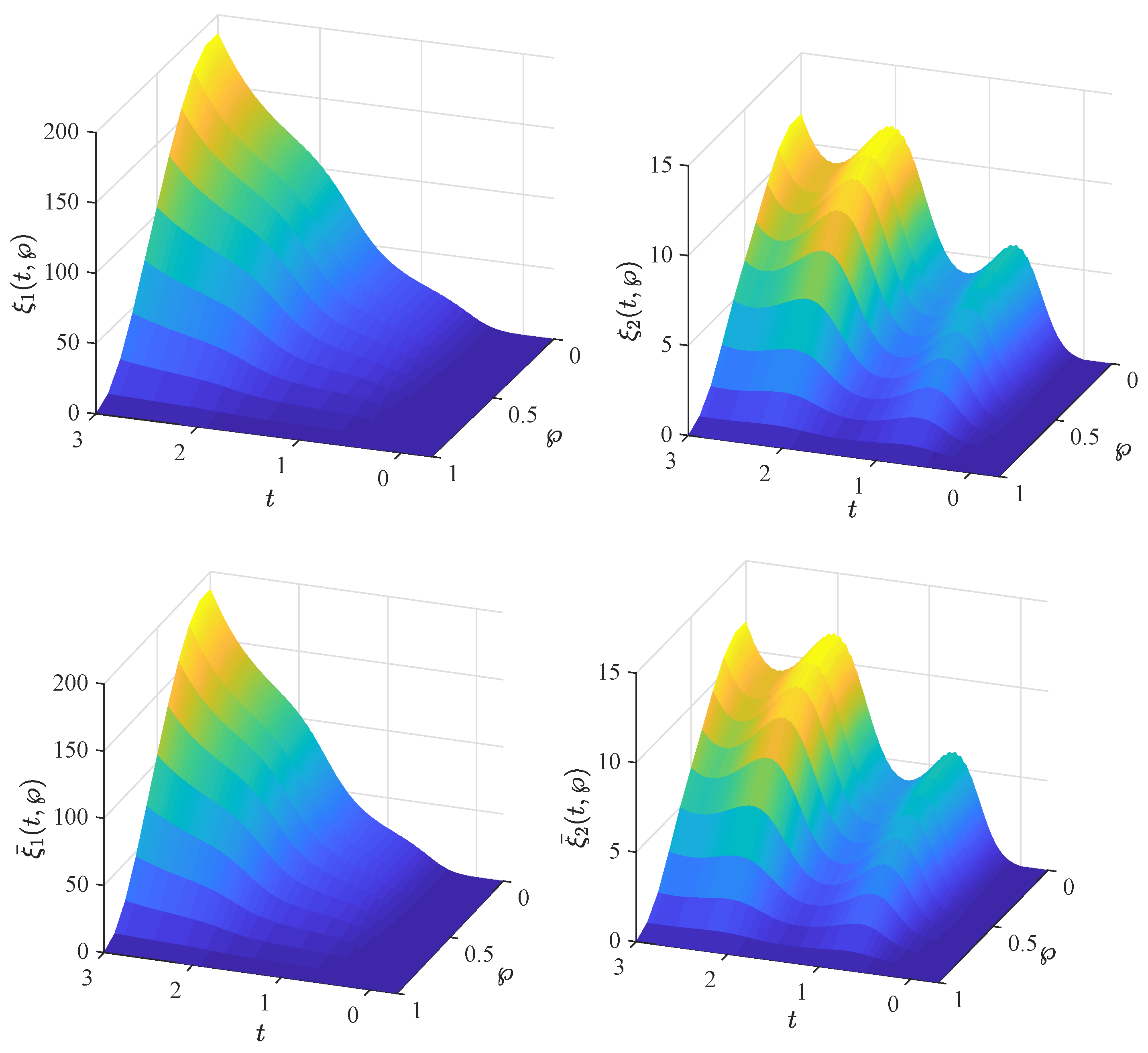
3. Global Asymptotic Stability via State Feedback Control

Definition 2.

The error system (4) is said to be globally asymptotically stable under the given controllers if

$$\underset{t\to \infty }{lim}\left({||\xi (\mathfrak{t},\wp )||}_1+||\overline{\xi }(\mathfrak{t},\wp ){||}_2\right)=0,$$

where ${||.||}_1$ and ${||.||}_2$ are the corresponding norms of $\xi (\mathfrak{t},\wp )={({\xi }_1(\mathfrak{t},\wp ),{\xi }_2(\mathfrak{t},\wp ),\cdots ,{\xi }_0(\mathfrak{t},\wp ))}^T\in {\mathbb{R}}^0$, and $\overline{\xi }(\mathfrak{t},\wp )={({\overline{\xi }}_1(\mathfrak{t},\wp ),{\overline{\xi }}_2(\mathfrak{t},\wp ),\cdots ,{\overline{\xi }}_n(\mathfrak{t},\wp ))}^T\in {\mathbb{R}}^n$, respectively.

Remark 1.

Since ${\xi }_{\phi }(\mathfrak{t},\wp )={\overline{\zeta }}_{\phi }(\mathfrak{t},\wp )-{\zeta }_{\phi }(\mathfrak{t},\wp )$, $\phi =1,2,\cdots ,o$ and ${\overline{\xi }}_{\varpi }(\mathfrak{t},\wp )={\overline{\Im }}_{\varpi }(\mathfrak{t},\wp )-{\Im }_{\varpi }(\mathfrak{t},\wp )$, $\varpi =1,2,\cdots ,n,$ the global asymptotic stability of the error system (4) is equivalent to a global asymptotic synchronization of the nodes of system (2) onto those of system (1) under the appropriate controllers.

Theorem 1.

Suppose that Assumptions 1–3 and the conditions of Lemma 6 hold, and ${\overline{M}}_{\phi },{\tilde{\overline{M}}}_{\varpi }$ are positive constants, such that ${\overline{M}}_{\phi }={\sum }_{k=1}^q\frac{m_{\phi k}}{l_k^2},{\tilde{\overline{M}}}_{\varpi }={\sum }_{k=1}^q\frac{{\tilde{m}}_{\varpi k}}{l_k^2}$. The error system (4) is globally asymptotically stable, if there exist constants $\rho >0$ and

$$\begin{array}{cc}\hfill {\mu }_{min}^{\left(1\right)}& =\underset{1\le \phi \le o}{min}\{2{\tilde{M}}_{\phi }+2d_{\phi }-\sum _{\varpi =1}^n|c_{\phi \varpi }|F_{\varpi }{\rho }^{-1}-\sum _{\varpi =1}^n|a_{\phi \varpi }|F_{\varpi }{\rho }^{-1}\hfill \\ & -\sum _{\varpi =1}^n|u_{\phi \varpi }|F_{\varpi }{\rho }^{-1}-\sum _{\varpi =1}^n|v_{\phi \varpi }|F_{\varpi }{\rho }^{-1}+t_{\phi }+{\psi }_{\phi }-\sum _{\varpi =1}^n|c_{\phi \varpi }|F_{\varpi }\rho \}>0,\hfill \\ \hfill {\mu }_{min}^{\left(2\right)}& =\underset{1\le \varpi \le n}{min}\{2{\overline{\tilde{M}}}_{\varpi }+2{\tilde{d}}_{\varpi }-\sum _{\phi =1}^o|{\tilde{c}}_{\varpi \phi }|G_{\phi }{\rho }^{-1}-\sum _{\phi =1}^o|{\tilde{a}}_{\varpi \phi }|G_{\phi }{\rho }^{-1}-\sum _{\phi =1}^o|{\tilde{u}}_{\varpi \phi }|G_{\phi }{\rho }^{-1}\hfill \\ & -\sum _{\phi =1}^o|{\tilde{v}}_{\varpi \phi }|G_{\phi }{\rho }^{-1}+{\varpi }_{\varpi }+{\varrho }_{\varpi }-\sum _{\phi =1}^o|{\tilde{c}}_{\varpi \phi }|G_{\phi }\rho \}>0,\hfill \\ \hfill {\Lambda }_1^{\mu }& =\underset{1\le \phi \le o}{max}\left\{\sum _{\varpi =1}^n|{\tilde{u}}_{\varpi \phi }|G_{\phi }\rho +\sum _{\varpi =1}^n|{\tilde{v}}_{\varpi \phi }|G_{\phi }\rho +\sum _{\varpi =1}^n|{\tilde{a}}_{\varpi \phi }|G_{\phi }\rho \right\}>0,\hfill \\ \hfill {\Lambda }_2^{\mu }& =\underset{1\le \varpi \le n}{max}\left\{\sum _{\phi =1}^o|u_{\phi \varpi }|F_{\varpi }\rho +\sum _{\phi =1}^o|v_{\phi \varpi }|F_{\varpi }\rho +\sum _{\phi =1}^o|a_{\phi \varpi }|F_{\varpi }\rho \right\}>0.\hfill \end{array}$$

such that

$$min\left\{{\mu }_{min}^{\left(1\right)},{\mu }_{min}^{\left(2\right)}\right\}>\sqrt{2}max\left\{{\Lambda }_1^{\mu },{\Lambda }_2^{\mu }\right\}.$$

Proof. 

We define a Lyapunov function as

$$\begin{array}{c}\hfill V\left(\mathfrak{t}\right)={\int }_{\Omega }\sum _{\phi =1}^o\frac{1}{2}{\xi }_{\phi }^2(\mathfrak{t},\wp )d\wp +{\int }_{\Omega }\sum _{\varpi =1}^n\frac{1}{2}{\overline{\xi }}_{\varpi }^2(\mathfrak{t},\wp )d\wp .\end{array}$$

(6)

Then, for the fractional derivative of V of order $\lambda$, we have

$$\begin{array}{cc}\hfill \frac{d^{\lambda }V\left(t\right)}{d{\mathfrak{t}}^{\lambda }}& =\frac{1}{2}\frac{d^{\lambda }}{d{\mathfrak{t}}^{\lambda }}\left({\int }_{\Omega }\frac{1}{2}\sum _{\phi =1}^o{\xi }_{\phi }^2(\mathfrak{t},\wp )d\wp +{\int }_{\Omega }\frac{1}{2}\sum _{\varpi =1}^n{\overline{\xi }}_{\varpi }^2(\mathfrak{t},\wp )d\wp \right)\hfill \\ \hfill & =\frac{1}{2}\sum _{\phi =1}^o\left[\frac{d^{\lambda }}{d{\mathfrak{t}}^{\lambda }}\left({\int }_{\Omega }{\xi }_{\phi }^2(\mathfrak{t},\wp )d\wp \right)\right]+\frac{1}{2}\sum _{\varpi =1}^n\left[\frac{d^{\lambda }}{d{t}^{\lambda }}\left({\int }_{\Omega }{\overline{\xi }}_{\varpi }^2(t,\wp )d\wp \right)\right].\hfill \end{array}$$

(7)

We have from Lemma 1 that

$$\begin{array}{cc}\hfill \frac{d^{\lambda }}{d{\mathfrak{t}}^{\lambda }}\left({\int }_{\Omega }{\xi }_{\phi }^2(\mathfrak{t},\wp )d\wp \right)& \le 2{\int }_{\Omega }{\xi }_{\phi }(\mathfrak{t},\wp )\frac{{\partial }^{\lambda }{\xi }_{\phi }(\mathfrak{t},\wp )}{\partial {\mathfrak{t}}^{\lambda }}d\wp ,\hfill \\ \hfill \frac{d^{\lambda }}{d{\mathfrak{t}}^{\lambda }}\left({\int }_{\Omega }{\overline{\xi }}_{\varpi }^2(\mathfrak{t},\wp )d\wp \right)& \le 2{\int }_{\Omega }{\overline{\xi }}_{\varpi }(\mathfrak{t},\wp )\frac{{\partial }^{\lambda }{\overline{\xi }}_{\varpi }(\mathfrak{t},\wp )}{\partial {\mathfrak{t}}^{\lambda }}d\wp .\hfill \end{array}$$

Substituting the above inequalities in Equation (7), we obtain

$$\begin{array}{cc}\hfill D^{\lambda }V\left(t\right))& \le \sum _{\phi =1}^o{\int }_{\Omega }{\xi }_{\phi }{(\mathfrak{t},\wp )}^C{D}^{\lambda }{\xi }_{\phi }(\mathfrak{t},\wp )d\wp +\sum _{\varpi =1}^n{\int }_{\Omega }{\tilde{\xi }}_{\varpi }{(\mathfrak{t},\wp )}^C{D}^{\lambda }{\tilde{\xi }}_{\varpi }(\mathfrak{t},\wp )d\wp \hfill \\ \hfill & =\sum _{\phi =1}^o{\int }_{\Omega }{\xi }_{\phi }(\mathfrak{t},\wp )(\sum _{k=1}^q\frac{\partial }{\partial {\zeta }_k}(m_{\phi k}\frac{\partial {\xi }_{\phi }\left(\mathfrak{t},\wp \right)}{\partial {\wp }_k})-d_{\phi }{\xi }_{\phi }\left(\mathfrak{t},\wp \right)\hfill \\ \hfill & +\left[\sum _{\varpi =1}^n{c}_{\phi \varpi }{f}_{\varpi }\left({\overline{\Im }}_{\varpi }\left(\mathfrak{t},\wp \right)\right)-\sum _{\varpi =1}^n{c}_{\phi \varpi }{f}_{\varpi }\left({\Im }_{\varpi }\left(\mathfrak{t},\wp \right)\right)\right]\hfill \\ \hfill & +\left[\sum _{\varpi =1}^n{a}_{\phi \varpi }{f}_{\varpi }\left({\overline{\Im }}_{\varpi }(\mathfrak{t}-\tau ,\wp )\right)-\sum _{\varpi =1}^n{a}_{\phi \varpi }{f}_{\varpi }\left({\Im }_{\varpi }(\mathfrak{t}-\tau ,\wp )\right)\right]\hfill \\ \hfill & +[\underset{\varpi =1}{\overset{n}{\bigwedge }}{u}_{\phi \varpi }{\int }_0^{\infty }{k}_{\phi \varpi }\left(s\right)f_{\varpi }\left({\overline{\Im }}_{\varpi }(s-\tau ,\wp )\right)ds\hfill \\ & -\underset{\varpi =1}{\overset{n}{\bigwedge }}{u}_{\phi \varpi }{\int }_0^{\infty }{k}_{\phi \varpi }\left(s\right)f_{\varpi }\left({\Im }_{\varpi }(s-\tau ,\wp )\right)ds]\hfill \\ \hfill & +[\underset{\varpi =1}{\overset{n}{\bigvee }}{v}_{\phi \varpi }{\int }_0^{\infty }{k}_{\phi \varpi }\left(s\right)f_{\varpi }\left({\overline{\Im }}_{\varpi }(s-\tau ,\wp )\right)ds\hfill \\ & -\underset{\varpi =1}{\overset{n}{\bigvee }}{v}_{\phi \varpi }{\int }_0^{\infty }{k}_{\phi \varpi }\left(s\right)f_{\varpi }\left({\Im }_{\varpi }(s-\tau ,\wp )\right)ds]\hfill \\ & -{\mathfrak{t}}_{\phi }{\xi }_{\phi }(\mathfrak{t},\wp )-{\Psi }_{\phi }{\xi }_{\phi }(\mathfrak{t},\wp ))d\wp \hfill \end{array}$$

$$\begin{array}{cc}\hfill & +\sum _{\varpi =1}^n{\int }_{\Omega }{\overline{\xi }}_{\varpi }(\mathfrak{t},\wp )(\sum _{k=1}^q\frac{\partial }{\partial {\Im }_k}({\tilde{m}}_{\varpi k}\frac{\partial {\overline{\xi }}_{\varpi }\left(\mathfrak{t},\wp \right)}{\partial {\wp }_k})-{\tilde{d}}_{\varpi }{\overline{\xi }}_{\varpi }\left(\mathfrak{t},\wp \right)\hfill \\ & +\left[\sum _{\phi =1}^o{\tilde{c}}_{\varpi \phi }{g}_{\phi }\left({\overline{\zeta }}_{\phi }(\mathfrak{t},\wp )\right)-\sum _{\phi =1}^o{\tilde{c}}_{\varpi \phi }{g}_{\phi }\left({\zeta }_{\phi }(\mathfrak{t},\wp )\right)\right]\hfill \\ & +\left[\sum _{\phi =1}^o{\tilde{a}}_{\varpi \phi }{g}_{\phi }\left({\overline{\zeta }}_{\phi }(\mathfrak{t}-\tau ,\wp )\right)-\sum _{\phi =1}^o{\tilde{a}}_{\varpi \phi }{g}_{\phi }\left({\zeta }_{\phi }(\mathfrak{t}-\tau ,\wp )\right)\right]\hfill \\ \hfill & +[\underset{\phi =1}{\overset{o}{\bigwedge }}{\tilde{u}}_{\varpi \phi }{\int }_0^{\infty }{k}_{\varpi \phi }\left(s\right)g_{\phi }\left({\overline{\zeta }}_{\phi }(s-\tau ,\wp )\right)ds\hfill \\ & -\underset{\phi =1}{\overset{o}{\bigwedge }}{\tilde{u}}_{\varpi \phi }{\int }_0^{\infty }{k}_{\varpi \phi }\left(s\right)g_{\phi }\left({\zeta }_{\phi }(s-\tau ,\wp )\right)ds]\hfill \\ & +[\underset{\phi =1}{\overset{o}{\bigvee }}{\tilde{v}}_{\varpi \phi }{\int }_0^{\infty }{k}_{\varpi \phi }\left(s\right)g_{\phi }\left({\overline{\zeta }}_{\phi }(s-\tau ,\wp )\right)ds\hfill \\ \hfill & -\underset{\phi =1}{\overset{o}{\bigvee }}{\tilde{v}}_{\varpi \phi }{\int }_0^{\infty }{k}_{\varpi \phi }\left(s\right)g_{\phi }\left({\zeta }_{\phi }(s-\tau ,\wp )\right)ds]\hfill \\ & -{\varpi }_{\varpi }{\tilde{\xi }}_{\varpi }(\mathfrak{t},\wp )-{\varrho }_{\varpi }{\tilde{\xi }}_{\varpi }(\mathfrak{t},\wp ))d\wp .\hfill \end{array}$$

By Green’s formula using the boundary conditions, we obtain

$$\begin{array}{c}\hfill \sum _{k=1}^q{\int }_{\Omega }{\xi }_{\phi }(\mathfrak{t},\wp )\frac{\partial }{\partial {\wp }_k}\left(m_{\phi k}\frac{\partial {\xi }_{\phi }(\mathfrak{t},\wp )}{\partial {\wp }_k}\right)d\wp =-\sum _{k=1}^q{\int }_{\Omega }{m}_{\phi k}{\left(\frac{\partial {\xi }_{\phi }(\mathfrak{t},\wp )}{\partial {\wp }_k}\right)}^{2}d\wp ,\end{array}$$

$$\begin{array}{c}\hfill \sum _{k=1}^q{\int }_{\Omega }{\overline{\xi }}_{\varpi }(\mathfrak{t},\wp )\frac{\partial }{\partial {\wp }_k}\left({\tilde{m}}_{\varpi k}\frac{\partial {\overline{\xi }}_{\varpi }(\mathfrak{t},\wp )}{\partial {\wp }_k}\right)d\wp =-\sum _{k=1}^q{\int }_{\Omega }{\tilde{m}}_{\varpi k}{\left(\frac{\partial {\overline{\xi }}_{\varpi }(\mathfrak{t},\wp )}{\partial {\wp }_k}\right)}^{2}d\wp .\end{array}$$

From the above identities and Lemma 6, we obtain

$$\begin{array}{cc}\hfill \sum _{k=1}^q{\int }_{\Omega }{\xi }_{\phi }(\mathfrak{t},\wp )\frac{\partial }{\partial {\wp }_k}\left(m_{\phi k}\frac{\partial {\xi }_{\phi }(\mathfrak{t},\wp )}{\partial {\wp }_k}\right)d\wp & =-\sum _{k=1}^q{\int }_{\Omega }{m}_{\phi k}{\left(\frac{\partial {\xi }_{\phi }(\mathfrak{t},\wp )}{\partial {\wp }_k}\right)}^{2}d\wp \hfill \\ \hfill & \le -\sum _{k=1}^q{\int }_{\Omega }\frac{m_{\phi k}}{l_k^2}{\xi }_{\phi }^2(\mathfrak{t},\wp )d\wp =-{\overline{M}}_{\phi }{\int }_{\Omega }{\xi }_{\phi }^2(\mathfrak{t},\wp )d\wp .\hfill \end{array}$$

Similarly,

$$\begin{array}{cc}\hfill \sum _{k=1}^q{\int }_{\Omega }{\overline{\xi }}_{\varpi }(\mathfrak{t},\wp )\frac{\partial }{\partial {\wp }_k}\left({\tilde{m}}_{\varpi k}\frac{\partial {\overline{\xi }}_{\varpi }(\mathfrak{t},\wp )}{\partial {\wp }_k}\right)d\wp & =-\sum _{k=1}^q{\int }_{\Omega }{\tilde{m}}_{\varpi k}{\left(\frac{\partial {\overline{\xi }}_{\varpi }(\mathfrak{t},\wp )}{\partial {\wp }_k}\right)}^{2}d\wp \hfill \\ \hfill & \le -\sum _{k=1}^q{\int }_{\Omega }\frac{{\tilde{m}}_{\varpi k}}{l_k^2}{\xi }_{\varpi }^2(\mathfrak{t},\wp )d\wp =-{\tilde{\overline{M}}}_{\varpi }{\int }_{\Omega }{\overline{\xi }}_{\varpi }^2(\mathfrak{t},\wp )d\wp .\hfill \end{array}$$

Then, using Assumptions 1 and 2, we obtain

$$\begin{array}{cc}\hfill D^{\lambda }V\left(\mathfrak{t}\right)& \le {\int }_{\Omega }\{-\sum _{\phi =1}^o{\overline{M}}_{\phi }{\xi }_{\phi }^2(\mathfrak{t},\wp )-\sum _{\phi =1}^o{d}_{\phi }{\xi }_{\phi }^2(\mathfrak{t},\wp )+\sum _{\phi =1}^o\sum _{\varpi =1}^n|c_{\phi \varpi }|F_{\varpi }|{\xi }_{\phi }(\mathfrak{t},\wp )||{\overline{\xi }}_{\varpi }(\mathfrak{t},\wp )|\hfill \\ \hfill & +\sum _{\phi =1}^o\sum _{\varpi =1}^n|a_{\phi \varpi }|F_{\varpi }|{\xi }_{\phi }(\mathfrak{t},\wp )||{\overline{\xi }}_{\varpi }(\mathfrak{t}-\tau ,\wp )|\hfill \\ & +\sum _{\phi =1}^o\sum _{\varpi =1}^n|u_{\phi \varpi }|{\int }_0^{\infty }{k}_{\phi \varpi }\left(s\right)F_{\varpi }|{\xi }_{\phi }(s,\wp )||{\tilde{\xi }}_{\varpi }(s-\tau ,\wp )|ds\hfill \\ & +\sum _{\phi =1}^o\sum _{\varpi =1}^n|v_{\phi \varpi }|{\int }_0^{\infty }{k}_{\phi \varpi }\left(s\right)F_{\varpi }|{\xi }_{\phi }(s,\wp )||{\overline{\xi }}_{\varpi }(s-\tau ,\wp )|ds-\sum _{\phi =1}^o{\mathfrak{t}}_{\phi }{\xi }_{\phi }^2(t,\wp )\hfill \\ & -\sum _{\phi =1}^o{\Psi }_{\phi }{\xi }_{\phi }^2(\mathfrak{t},\wp )-\sum _{\varpi =1}^n{\overline{\tilde{M}}}_{\varpi }{\overline{\xi }}_{\varpi }^2(\mathfrak{t},\wp )-\sum _{\varpi =1}^n{\tilde{d}}_{\varpi }{\overline{\xi }}_{\varpi }^2(\mathfrak{t},\wp )\hfill \\ & +\sum _{\varpi =1}^n\sum _{\phi =1}^o|{\tilde{c}}_{\varpi \phi }|G_{\phi }|{\overline{\xi }}_{\varpi }(\mathfrak{t},\wp )||{\xi }_{\phi }(\mathfrak{t},\wp )|\hfill \\ & +\sum _{\varpi =1}^n\sum _{\phi =1}^o|{\tilde{a}}_{\varpi \phi }|G_{\phi }|{\overline{\xi }}_{\varpi }(\mathfrak{t},\wp )||{\xi }_{\phi }(\mathfrak{t}-\tau ,\wp )|\hfill \\ & +\sum _{\varpi =1}^n\sum _{\phi =1}^o|{\tilde{u}}_{\varpi \phi }|{\int }_0^{\infty }{k}_{\varpi \phi }\left(s\right)G_{\phi }{\overline{\xi }}_{\varpi }(s,\wp )||{\xi }_{\phi }(s-\tau ,\wp )|ds\hfill \\ & +\sum _{\varpi =1}^n\sum _{\phi =1}^o|{\tilde{v}}_{\varpi \phi }|{\int }_0^{\infty }{k}_{\varpi \phi }\left(s\right)G_{\phi }{\overline{\xi }}_{\varpi }(s,\wp )|{\xi }_{\phi }(s-\tau ,\wp )|ds\hfill \\ & -\sum _{\phi =1}^o{\varpi }_{\varpi }{\tilde{\xi }}_{\phi }^2(\mathfrak{t},\wp )-\sum _{\phi =1}^o{\varrho }_{\varpi }{\overline{\xi }}_{\phi }^2(\mathfrak{t},\wp )\}d\wp .\hfill \end{array}$$

Lemma 5 implies the existence of a constant $\rho >0$ such that

$$\begin{array}{cc}\hfill D^{\lambda }V\left(\mathfrak{t}\right)& \le {\int }_{\Omega }\{-\sum _{\phi =1}^o{\overline{M}}_{\phi }{\xi }_{\phi }^2(\mathfrak{t},\wp )-\sum _{\phi =1}^o{d}_{\phi }{\xi }_{\phi }^2(\mathfrak{t},\wp )+\sum _{\phi =1}^o\sum _{\varpi =1}^n|c_{\phi \varpi }|F_{\varpi }[\frac{{\rho }^{-1}}{2}{\xi }_{\phi }^2(\mathfrak{t},\wp )+\frac{\rho }{2}{\overline{\xi }}_{\varpi }^2(\mathfrak{t},\wp )]\hfill \\ \hfill & +\sum _{\phi =1}^o\sum _{\varpi =1}^n|a_{\phi \varpi }|F_{\varpi }[\frac{{\rho }^{-1}}{2}{\xi }_{\phi }^2(\mathfrak{t},\wp )+\frac{\rho }{2}{\overline{\xi }}_{\varpi }^2(\mathfrak{t}-\tau ,\wp )]\hfill \\ \hfill & +\sum _{\phi =1}^o\sum _{\varpi =1}^n|u_{\phi \varpi }|{\int }_0^{\infty }{k}_{\phi \varpi }\left(s\right)F_{\varpi }[\frac{{\rho }^{-1}}{2}{\xi }_{\phi }^2(s,\wp )+\frac{\rho }{2}{\overline{\xi }}_{\varpi }^2(s-\tau ,\wp )]ds\hfill \\ \hfill & +\sum _{\phi =1}^o\sum _{\varpi =1}^n|v_{\phi \varpi }|{\int }_0^{\infty }{k}_{\phi \varpi }\left(s\right)F_{\varpi }[\frac{{\rho }^{-1}}{2}{\xi }_{\phi }^2(s,\wp )+\frac{\rho }{2}{\overline{\xi }}_{\varpi }^2(s-\tau ,\wp )]ds\hfill \\ \hfill & -\sum _{\phi =1}^o{\mathfrak{t}}_{\phi }{\xi }_{\phi }^2(\mathfrak{t},\wp )-\sum _{\phi =1}^o{\Psi }_{\phi }{\xi }_{\phi }^2(\mathfrak{t},\wp )\hfill \\ \hfill & -\sum _{\varpi =1}^n{\overline{\tilde{M}}}_{\varpi }{\overline{\xi }}_{\varpi }^2(\mathfrak{t},\wp )-\sum _{\varpi =1}^n{\tilde{d}}_{\varpi }{\overline{\xi }}_{\varpi }^2(\mathfrak{t},\wp )+\sum _{\varpi =1}^n\sum _{\phi =1}^o|{\tilde{c}}_{\varpi \phi }|G_{\phi }[\frac{{\rho }^{-1}}{2}{\overline{\xi }}_{\varpi }^2(\mathfrak{t},\wp )+\frac{\rho }{2}{\xi }_{\phi }^2(\mathfrak{t},\wp )]\hfill \\ & +\sum _{\varpi =1}^n\sum _{\phi =1}^o|{\tilde{a}}_{\varpi \phi }|G_{\phi }[\frac{{\rho }^{-1}}{2}{\overline{\xi }}_{\varpi }^2(\mathfrak{t},\wp )+\frac{\rho }{2}{\xi }_{\phi }^2(\mathfrak{t}-\tau ,\wp )]\hfill \end{array}$$

$$\begin{array}{cc}& +\sum _{\varpi =1}^n\sum _{\phi =1}^o|{\tilde{u}}_{\varpi \phi }|{\int }_0^{\infty }{k}_{\varpi \phi }\left(s\right)G_{\phi }[\frac{{\rho }^{-1}}{2}{\overline{\xi }}_{\varpi }^2(s,\wp )+\frac{\rho }{2}{\xi }_{\phi }^2(s-\tau ,\wp )]ds\hfill \\ & +\sum _{\varpi =1}^n\sum _{\phi =1}^o|{\tilde{v}}_{\varpi \phi }|{\int }_0^{\infty }{k}_{\varpi \phi }\left(s\right)G_{\phi }[\frac{{\rho }^{-1}}{2}{\overline{\xi }}_{\varpi }^2(s,\wp )+\frac{\rho }{2}{\xi }_{\phi }^2(s-\tau ,\wp )]ds\hfill \\ & -\sum _{\varpi =1}^n{\varpi }_{\varpi }{\overline{\xi }}_{\phi }^2(\mathfrak{t},\wp )-\sum _{\varpi =1}^n{\varrho }_{\varpi }{\overline{\xi }}_{\phi }^2(t,\wp )\}.\hfill \end{array}$$

We apply Assumption 3 to obtain

$$\begin{array}{cc}\hfill D^{\lambda }V\left(\mathfrak{t}\right)& \le {\int }_{\Omega }{\xi }_{\phi }^2(\mathfrak{t},\wp )\{-\sum _{\phi =1}^o{\tilde{M}}_{\phi }-\sum _{\phi =1}^o{d}_{\phi }+\sum _{\phi =1}^o\sum _{\varpi =1}^n|c_{\phi \varpi }|F_{\varpi }\frac{{\rho }^{-1}}{2}+\sum _{\phi =1}^o\sum _{\varpi =1}^n|a_{\phi \varpi }|F_{\varpi }\frac{{\rho }^{-1}}{2}\hfill \\ & +\sum _{\phi =1}^o\sum _{\varpi =1}^n|u_{\phi \varpi }|F_{\varpi }\frac{{\rho }^{-1}}{2}+\sum _{\phi =1}^o\sum _{\varpi =1}^n|v_{\phi \varpi }|F_{\varpi }\frac{{\rho }^{-1}}{2}-\sum _{\phi =1}^o{\mathfrak{t}}_{\phi }-\sum _{\phi =1}^o{\Psi }_{\phi }+\sum _{\varpi =1}^n\sum _{\phi =1}^o|{\tilde{c}}_{\varpi \phi }|G_{\phi }\frac{\rho }{2}\}\hfill \\ & +\underset{-\infty <\mathfrak{s}\le 0}{max}{\xi }_{\phi }^2(\mathfrak{s},\wp )\left\{\sum _{\varpi =1}^n\sum _{\phi =1}^o|{\tilde{a}}_{\varpi \phi }|G_{\phi }\frac{\rho }{2}+\sum _{\varpi =1}^n\sum _{\phi =1}^o|{\tilde{v}}_{\varpi \phi }|G_{\phi }\frac{\rho }{2}+\sum _{\varpi =1}^n\sum _{\phi =1}^o|{\tilde{u}}_{\varpi \phi }|G_{\phi }\frac{\rho }{2}\right\}\hfill \\ & +{\overline{\xi }}_{\varpi }^2(\mathfrak{t},\wp )\{-\sum _{\varpi =1}^n{\overline{\tilde{M}}}_{\varpi }-\sum _{\varpi =1}^n{\tilde{d}}_{\varpi }+\sum _{\varpi =1}^n\sum _{\phi =1}^o|{\tilde{c}}_{\varpi \phi }|G_{\phi }\frac{{\rho }^{-1}}{2}+\sum _{\varpi =1}^n\sum _{\phi =1}^o|{\tilde{a}}_{\varpi \phi }|G_{\phi }\frac{{\rho }^{-1}}{2}\hfill \\ & +\sum _{\varpi =1}^n\sum _{\phi =1}^o|{\tilde{u}}_{\varpi \phi }|G_{\phi }\frac{{\rho }^{-1}}{2}+\sum _{\varpi =1}^n\sum _{\phi =1}^o|{\tilde{v}}_{\varpi \phi }|G_{\phi }\frac{{\rho }^{-1}}{2}-\sum _{\varpi =1}^n{\varpi }_{\varpi }-\sum _{\varpi =1}^n{\varrho }_{\varpi }\hfill \\ & +\sum _{\phi =1}^o\sum _{\varpi =1}^n|{\tilde{c}}_{\phi \varpi }|G_{\phi }\frac{\rho }{2}\}+\underset{-\infty <\mathfrak{s}\le 0}{max}{\overline{\xi }}_{\varpi }^2(\mathfrak{s},\wp )\{\sum _{\phi =1}^o\sum _{\varpi =1}^n|u_{\phi \varpi }|F_{\phi }\frac{\rho }{2}\hfill \\ & +\sum _{\phi =1}^o\sum _{\varpi =1}^n|v_{\phi \varpi }|F_{\phi }\frac{\rho }{2}+\sum _{\phi =1}^o\sum _{\varpi =1}^n|a_{\phi \varpi }|F_{\phi }\frac{\rho }{2}\}d\wp ,\hfill \end{array}$$

or

$$\begin{array}{cc}\hfill D^{\lambda }V\left(\mathfrak{t}\right)& \le {\int }_{\Omega }\{-{\mu }_{min}^{\left(1\right)}\sum _{\phi =1}^o{\xi }_{\phi }^2(\mathfrak{t},\wp )-{\mu }_{min}^{\left(2\right)}\sum _{\varpi =1}^n{\overline{\xi }}_{\varpi }^2(\mathfrak{t},\wp )+{\Omega }_{max}^{\left(1\right)}\sum _{\phi =1}^n\underset{-\infty <\mathfrak{s}\le 0}{max}{\xi }_{\phi }^2(\mathfrak{s},\wp )\hfill \\ & +{\Omega }_{max}^{\left(2\right)}\sum _{\phi =1}^n\underset{-\infty <\mathfrak{s}\le 0}{max}{\overline{\xi }}_{\varpi }^2(\mathfrak{s},\wp )\}d\wp \le -\mu V\left(t\right)+\Lambda \underset{-\infty <\mathfrak{s}\le 0}{max}V\left(\mathfrak{s}\right),\hfill \end{array}$$

where $\mu =min\left\{{\mu }_{min}^{\left(1\right)},{\mu }_{min}^{\left(2\right)}\right\}$, and $\Lambda =max\left\{{\Lambda }_1^{\mu },{\Lambda }_2^{\mu }\right\}.$

By Lemma 3, since $\mu >\sqrt{2}\Lambda$, we have ${lim}_{\mathfrak{t}\to \infty }V\left(\mathfrak{t}\right)=0$.

For ${||\xi (\mathfrak{t},\wp )||}_1+||\overline{\xi }(\mathfrak{t},\wp ){||}_2=V\left(\mathfrak{t}\right)$, we can conclude that system (4) is globally asymptotically stable. This means that the drive system (1) and the response system (2) are globally asymptotically synchronized via the state feedback controllers. This completes the proof of the theorem. □

Remark 2.

Different from all existent synchronization results for neural network models, we consider a class of more general structures which include Caputo type fractional derivatives, reaction–diffusion terms, discrete and distributed delays which allow us to divide all nodes in the network into different classes, a BAM two-layer connection, fuzzy logic, and hybrid feedback controllers. Thus, the proposed results in Theorem 1 generalize and complement numerous asymptotic synchronization results. For example, our results generalize the results in [16] to the BAM case considering Caputo’s fractional differential operators. Moreover, the results established complement the results in [2] considering Caputo’s fractional differential operators and hybrid feedback controllers.

Remark 3.

The proposed global asymptotic synchronization criteria in Theorem 1 are in the forms of inequalities between the system parameters. This form allows applied researchers to easily apply the established results. The presence of the terms that include $|u_{\phi \varpi }|$, $|v_{\phi \varpi }|$, $|{\tilde{u}}_{\varpi \phi }|$, and $|{\tilde{v}}_{\varpi \phi }|$ in the conditions for ${\mu }_{min}^{\left(1\right)}$, ${\mu }_{min}^{\left(2\right)}$, ${\Lambda }_1^{\mu }$, and ${\Lambda }_2^{\mu }$ reflects the role of the distributed delays with delay kernels which satisfy Assumption 3. Furthermore, the terms $t_{\phi }+{\psi }_{\phi }$ and ${\varpi }_{\varpi }+{\varrho }_{\varpi }$ reflect the design of the controllers.

Remark 4.

Without feedback controllers, the error system (4) becomes

$$\begin{array}{cc}\hfill \frac{{\partial }^{\lambda }{\xi }_{\phi }\left(\mathfrak{t},\wp \right)}{\partial {\mathfrak{t}}^{\lambda }}& =\sum _{k=1}^q\frac{\partial }{\partial {\wp }_k}\left(m_{\phi k}\frac{\partial {\xi }_{\phi }\left(\mathfrak{t},\wp \right)}{\partial {\wp }_k}\right)-d_{\phi }{\xi }_{\phi }\left(\mathfrak{t},\wp \right)\hfill \\ & +\left[\sum _{\varpi =1}^n{c}_{\phi \varpi }{f}_{\varpi }\left({\overline{\Im }}_{\varpi }\left(\mathfrak{t},\wp \right)\right)-\sum _{\varpi =1}^n{c}_{\phi \varpi }{f}_{\varpi }\left({\Im }_{\varpi }\left(\mathfrak{t},\wp \right)\right)\right]\hfill \\ & +\left[\sum _{\varpi =1}^n{a}_{\phi \varpi }{f}_{\varpi }\left({\overline{\Im }}_{\varpi }(\mathfrak{t}-\tau ,\wp )\right)-\sum _{\varpi =1}^n{a}_{\phi \varpi }{f}_{\varpi }\left({\Im }_{\varpi }(t-\tau ,\wp )\right)\right]\hfill \\ & +[\underset{\varpi =1}{\overset{n}{\bigwedge }}{u}_{\phi \varpi }{\int }_0^{\infty }{k}_{\phi \varpi }\left(s\right)f_{\varpi }\left({\overline{\Im }}_{\varpi }(s-\tau ,\wp )\right)ds\hfill \\ & -\underset{\varpi =1}{\overset{n}{\bigwedge }}{u}_{\phi \varpi }{\int }_0^{\infty }{k}_{\phi \varpi }\left(s\right)f_{\varpi }\left({\Im }_{\varpi }(s-\tau ,\wp )\right)ds]\hfill \\ & +[\underset{\varpi =1}{\overset{n}{\bigvee }}{v}_{\phi \varpi }{\int }_0^{\infty }{k}_{\phi \varpi }\left(s\right)f_{\varpi }\left({\overline{\Im }}_{\varpi }(s-\tau ,\wp )\right)ds\hfill \\ & -\underset{\varpi =1}{\overset{n}{\bigvee }}{v}_{\phi \varpi }{\int }_0^{\infty }{k}_{\phi \varpi }\left(s\right)f_{\varpi }\left({\Im }_{\varpi }(s-\tau ,\wp )\right)ds],\phi =1,2,\dots ,o,\hfill \end{array}$$

$$\begin{array}{cc}\hfill \frac{{\partial }^{\lambda }{\overline{\xi }}_{\varpi }\left(\mathfrak{t},\wp \right)}{\partial {\mathfrak{t}}^{\lambda }}& =\sum _{k=1}^q\frac{\partial }{\partial {\wp }_k}\left({\tilde{m}}_{\varpi k}\frac{\partial {\overline{\xi }}_{\varpi }\left(\mathfrak{t},\wp \right)}{\partial {\wp }_k}\right)-{\tilde{d}}_{\varpi }{\overline{\xi }}_{\varpi }\left(\mathfrak{t},\wp \right)\hfill \\ & +\left[\sum _{\phi =1}^o{\tilde{c}}_{\varpi \phi }{g}_{\phi }\left({\overline{\zeta }}_{\phi }(t,\wp )\right)-\sum _{\phi =1}^o{\tilde{c}}_{\varpi \phi }{g}_{\phi }\left({\zeta }_{\phi }(t,\wp )\right)\right]\hfill \\ & +\left[\sum _{\phi =1}^o{\tilde{a}}_{\varpi \phi }{g}_{\phi }\left({\overline{\zeta }}_{\phi }(\mathfrak{t}-\tau ,\wp )\right)-\sum _{\phi =1}^o{\tilde{a}}_{\varpi \phi }{g}_{\phi }\left({\zeta }_{\phi }(\mathfrak{t}-\tau ,\wp )\right)\right]\hfill \\ & +[\underset{\phi =1}{\overset{o}{\bigwedge }}{\tilde{u}}_{\varpi \phi }{\int }_0^{\infty }{k}_{\varpi \phi }\left(s\right)g_{\phi }\left({\overline{\zeta }}_{\phi }(s-\tau ,\wp )\right)ds\hfill \\ & -\underset{\phi =1}{\overset{o}{\bigwedge }}{\tilde{u}}_{\varpi \phi }{\int }_0^{\infty }{k}_{\varpi \phi }\left(s\right)g_{\phi }\left({\overline{\zeta }}_{\phi }(s-\tau ,\wp )\right)ds]\hfill \\ & +[\underset{\phi =1}{\overset{o}{\bigvee }}{\tilde{v}}_{\varpi \phi }{\int }_0^{\infty }{k}_{\varpi \phi }\left(s\right)g_{\phi }\left({\overline{\zeta }}_{\phi }(s-\tau ,\wp )\right)ds\hfill \\ & -\underset{\phi =1}{\overset{o}{\bigvee }}{\tilde{v}}_{\varpi \phi }{\int }_0^{\infty }{k}_{\varpi \phi }\left(s\right)g_{\phi }\left({\zeta }_{\phi }(s-\tau ,\wp )\right)ds],\varpi =1,2,\dots ,n.\hfill \end{array}$$

(8)

Theorem 2.

Suppose that Assumptions 1–3, $\tau <1$, and conditions of Lemma 6 hold. The error system (8) is globally asymptotically stable, if there exist constants

$$\begin{array}{cc}\hfill {\Theta }_1& =\underset{1\le \phi \le o}{min}\left\{({\tilde{M}}_{\phi }+d_{\phi })-\sum _{\varpi =1}^n|{\tilde{c}}_{\varpi \phi }|G_{\phi }\right\}>0,\hfill \\ \hfill {\Theta }_2& =\underset{1\le \phi \le o}{min}\left\{({\overline{\tilde{M}}}_{\varpi }+{\tilde{d}}_{\varpi })-\sum _{\phi =1}^o|c_{\phi \varpi }|F_{\varpi }\right\}>0,\hfill \\ \hfill {\Lambda }_1^{\theta }& =\left\{\sum _{\varpi =1}^n\sum _{\phi =1}^o|{\tilde{a}}_{\varpi \phi }|G_{\phi }+\sum _{\varpi =1}^n\sum _{\phi =1}^o|{\tilde{u}}_{\varpi \phi }|G_{\phi }+\sum _{\varpi =1}^n\sum _{\phi =1}^o|{\tilde{v}}_{\varpi \phi }|G_{\phi }\right\}>0,\hfill \\ \hfill {\Lambda }_2^{\theta }& =\left\{\sum _{\phi =1}^o\sum _{\varpi =1}^n|a_{\phi \varpi }|F_{\varpi }+\sum _{\phi =1}^o\sum _{\varpi =1}^n|u_{\varpi \phi }|F_{\varpi }+\sum _{\phi =1}^o\sum _{\varpi =1}^n|v_{\varpi \phi }|F_{\varpi }\right\}>0,\hfill \end{array}$$

such that

$$min\left\{{\Theta }_1,{\Theta }_2\right\}>max\left\{{\Lambda }_1^{\theta },{\Lambda }_2^{\theta }\right\}.$$

Proof. 

We define a Lyapunov function as

$$\begin{array}{cc}\hfill V\left(\mathfrak{t}\right)& ={\int }_{\Omega }{D}^{-(1-\lambda )}\left[\sum _{\phi =1}^o|{\xi }_{\phi }(\mathfrak{t},\wp )|+\sum _{\varpi =1}^n|{\overline{\xi }}_{\varpi }(\mathfrak{t},\wp )|\right]d\wp +{\int }_{\Omega }\sum _{\phi =1}^o{\int }_{\mathfrak{t}-\tau }^{\mathfrak{t}}|{\xi }_{\phi }(s,\wp )|dsd\wp \hfill \\ & +{\int }_{\Omega }\sum _{\varpi =1}^n{\int }_{\mathfrak{t}-\tau }^{\mathfrak{t}}|{\overline{\xi }}_{\varpi }(s,\wp )|dsd\wp .\hfill \end{array}$$

(9)

Taking the time derivative of (9), we obtain

$$\begin{array}{cc}\hfill \frac{dV\left(\mathfrak{t}\right)}{d\mathfrak{t}}& ={\int }_{\Omega }{D}^{\lambda }\left[\sum _{\phi =1}^o|{\xi }_{\phi }(\mathfrak{t},\wp )|+\sum _{\varpi =1}^n|{\overline{\xi }}_{\varpi }(\mathfrak{t},\wp )|\right]d\wp +{\int }_{\Omega }\sum _{\phi =1}^o|{\xi }_{\phi }(\mathfrak{t},\wp )|d\wp -{\int }_{\Omega }\sum _{\phi =1}^o|{\xi }_{\phi }(\mathfrak{t}-\tau ,\wp )|d\wp \hfill \\ & +{\int }_{\Omega }\sum _{\varpi =1}^n|{\overline{\xi }}_{\varpi }(\mathfrak{t},\wp )|d\wp -{\int }_{\Omega }\sum _{\varpi =1}^n|{\overline{\xi }}_{\varpi }(\mathfrak{t}-{\tau }_1\left(t\right),\wp )|d\wp .\hfill \end{array}$$

The rest of the proof is similar to the proof of Theorem 1. Instead of Lemma 3, the fractional Barbalat’s Lemma is used. □

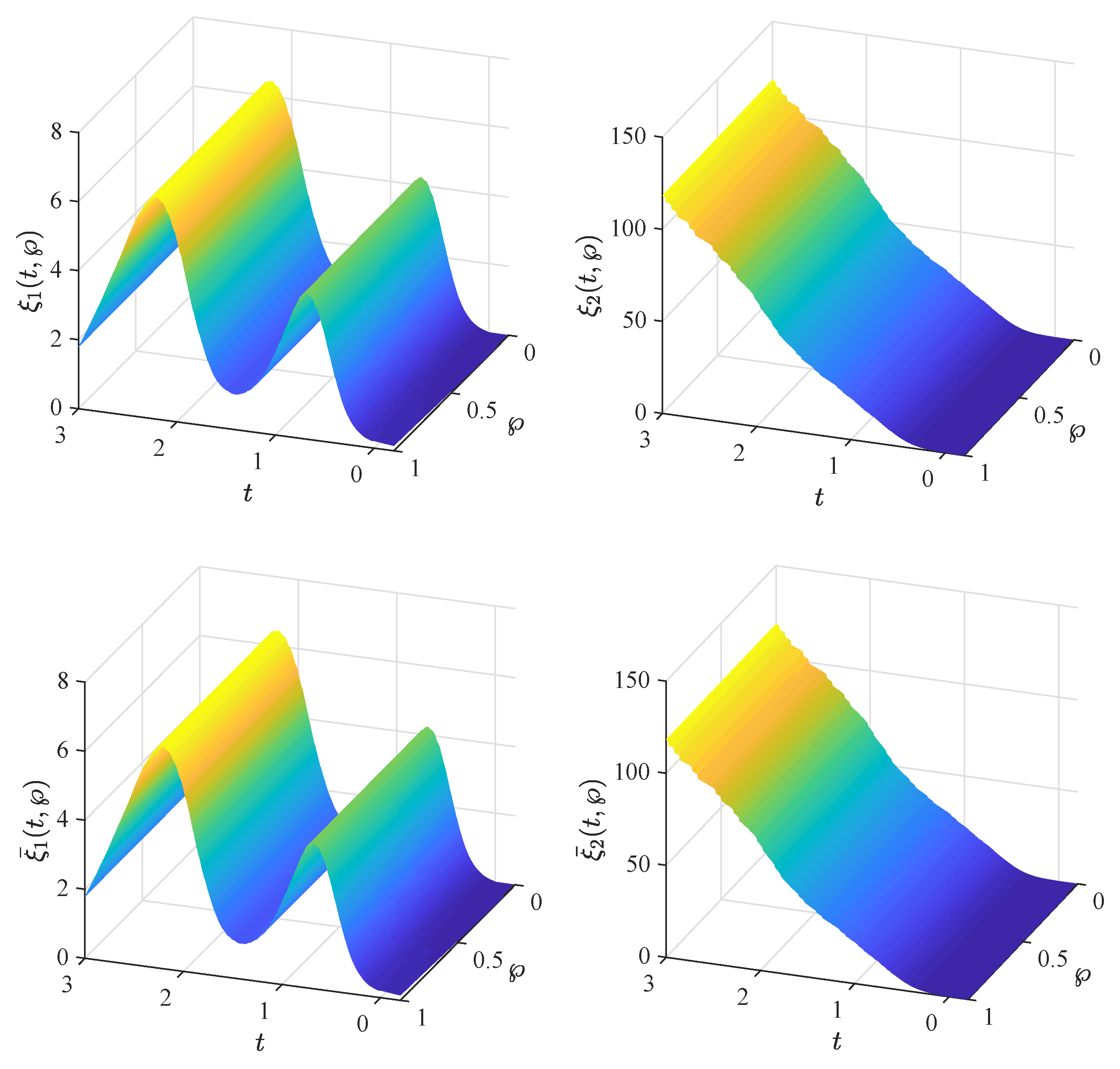
4. Global Mittag–Leffler Synchronization

For fractional-order systems, the concept of Mittag–Leffler stability was introduced in [23]. This notion generalizes the exponential stability notion for integer-order systems and has been investigated intensively [23,24,25,26,27,28,29,34,44]. In this section, we establish criteria for the global Mittag–Leffler stability of the error system (8).

Definition 3.

The error system (8) is said to be globally Mittag–Leffler stable, if for any continuous initial functions ϕ, ${({\varphi }_1,{\varphi }_2,\cdots ,{\varphi }_o)}^T$ and $\tilde{\varphi }$, ${({\tilde{\varphi }}_1,{\tilde{\varphi }}_2,\cdots ,{\tilde{\varphi }}_n)}^T$, there exist positive constants δ and q such that

$$\begin{array}{c}\hfill {||\xi (\mathfrak{t},\wp )||}_1+||\overline{\xi }(\mathfrak{t},\wp ){||}_2\le {\left\{{M(||\varphi ||}_{\infty }^1+||\tilde{\varphi }{||}_{\infty }^2)E_{\lambda }(-\delta t^{\lambda })\right\}}^q\end{array}$$

for $t\ge 0$, where $E_{\lambda }$ is the corresponding Mittag–Leffler function, ${||\varphi ||}_{\infty }^1={max}_{\mathfrak{s}\in (-\infty ,0]}{||\varphi \left(\mathfrak{s}\right)||}_1$, $||\tilde{\varphi }{||}_{\infty }^2={max}_{\mathfrak{s}\in (-\infty ,0]}||\tilde{\varphi }\left(\mathfrak{s}\right){||}_2$, $M\left(0\right)=0$, $M\ge 0$, and M is Lipschitz with respect to its argument.

The global Mittag–Lefler stability of the error system (8) is equivalent to the global Mittag–Leffler synchronization of the master and response systems.

Theorem 3.

Suppose that Assumptions 1–3 and the conditions of Lemma 6 hold. The error system (8) is globally Mittag–Leffler stable if there exist constants $\rho >0$ and

$$\begin{array}{cc}\hfill {\nu }_{min}^{\left(1\right)}& =\underset{1\le \phi \le o}{min}\{2{\tilde{M}}_{\phi }+2d_{\phi }-\sum _{\varpi =1}^n|c_{\phi \varpi }|F_{\varpi }{\rho }^{-1}-\sum _{\varpi =1}^n|a_{\phi \varpi }|F_{\varpi }{\rho }^{-1}\hfill \\ & -\sum _{\varpi =1}^n|u_{\phi \varpi }|F_{\varpi }{\rho }^{-1}-\sum _{\varpi =1}^n|v_{\phi \varpi }|F_{\varpi }{\rho }^{-1}-\sum _{\varpi =1}^n|c_{\phi \varpi }|F_{\varpi }\rho \}>0,\hfill \\ \hfill {\nu }_{min}^{\left(2\right)}& =\underset{1\le \varpi \le n}{min}\{2{\overline{\tilde{M}}}_{\varpi }+2{\tilde{d}}_{\varpi }-\sum _{\phi =1}^o|{\tilde{c}}_{\varpi \phi }|G_{\phi }{\rho }^{-1}-\sum _{\phi =1}^o|{\tilde{a}}_{\varpi \phi }|G_{\phi }{\rho }^{-1}-\sum _{\phi =1}^o|{\tilde{u}}_{\varpi \phi }|G_{\phi }{\rho }^{-1}\hfill \\ & -\sum _{\phi =1}^o|{\tilde{v}}_{\varpi \phi }|G_{\phi }{\rho }^{-1}-\sum _{\phi =1}^o|{\tilde{c}}_{\varpi \phi }|G_{\phi }\rho \}>0,\hfill \\ \hfill {\Lambda }_1^{\nu }& =\underset{1\le \phi \le o}{max}\left\{\sum _{\varpi =1}^n|{\tilde{u}}_{\varpi \phi }|G_{\phi }\rho +\sum _{\varpi =1}^n|{\tilde{v}}_{\varpi \phi }|G_{\phi }\rho +\sum _{\varpi =1}^n|{\tilde{a}}_{\varpi \phi }|G_{\phi }\rho \right\}>0,\hfill \\ \hfill {\Lambda }_2^{\nu }& =\underset{1\le \varpi \le n}{max}\left\{\sum _{\phi =1}^o|u_{\phi \varpi }|F_{\varpi }\rho +\sum _{\phi =1}^o|v_{\phi \varpi }|F_{\varpi }\rho +\sum _{\phi =1}^o|a_{\phi \varpi }|F_{\varpi }\rho \right\}>0,\hfill \end{array}$$

such that

$$min\left\{{\nu }_{min}^{\left(1\right)},{\nu }_{min}^{\left(2\right)}\right\}\ge max\left\{{\Lambda }_1^{\nu },{\Lambda }_2^{\nu }\right\}.$$

Proof. 

We define again a Lyapunov function as

$$\begin{array}{c}\hfill V\left(\mathfrak{t}\right)={\int }_{\Omega }\sum _{\phi =1}^o\frac{1}{2}{\xi }_{\phi }^2(\mathfrak{t},\wp )d\wp +{\int }_{\Omega }\sum _{\varpi =1}^n\frac{1}{2}{\overline{\xi }}_{\varpi }^2(\mathfrak{t},\wp )d\wp .\end{array}$$

(10)

Applying the same technique and steps as in the proof of Theorem 1, we obtain

$$\begin{array}{cc}\hfill D^{\lambda }V\left(\mathfrak{t}\right)& \le -\nu V\left(t\right)+\Lambda \underset{-\infty <\mathfrak{s}\le 0}{max}V\left(\mathfrak{s}\right),\hfill \end{array}$$

where $\nu =min\left\{{\nu }_{min}^{\left(1\right)},{\nu }_{min}^{\left(2\right)}\right\}$ and $\Lambda =max\left\{{\Lambda }_1^{\mu },{\Lambda }_2^{\mu }\right\}.$

We apply the Razumikhin condition

$$\begin{array}{c}\hfill V\left(\mathfrak{s}\right)\le V\left(\mathfrak{t}\right),-\infty <\mathfrak{s}\le \mathfrak{t}\end{array}$$

(11)

to the above inequality to obtain

$$\begin{array}{c}\hfill D^{\lambda }V\left(\mathfrak{t}\right)\le -(\nu -\Lambda )V\left(\mathfrak{t}\right).\end{array}$$

Since $\nu \ge \Lambda$, there exists a positive constant $\delta$, such that

$$\begin{array}{c}\hfill D^{\lambda }V\left(\mathfrak{t}\right)\le -\delta V\left(\mathfrak{t}\right).\end{array}$$

Then, by Lemma 2, we have

$$\begin{array}{c}\hfill {\displaystyle V\left(\mathfrak{t}\right)\le \underset{-\infty <\mathfrak{s}\le 0}{max}V\left(\mathfrak{s}\right)E_{\lambda }(-\delta t^{\lambda }),\mathfrak{t}>0.}\end{array}$$

Therefore,

$$\begin{array}{c}\hfill {||\xi (\mathfrak{t},\wp )||}_1+||\overline{\xi }(\mathfrak{t},\wp ){||}_2\le \left({||\varphi ||}_{\infty }^1+||\tilde{\varphi }{||}_{\infty }^2\right)E_{\lambda }(-\delta t^{\lambda }),\end{array}$$

i.e., according to Definition 3, the error system (8) is globally Mittag–Leffler stable, which means that the master and response systems are globally Mittag–Leffler synchronized. The proof is completed. □

Remark 5.

When the distributed delays and diffusion terms are not considered in model (1), the fractional-order fuzzy BAM neural network is denoted as follows:

$$\begin{array}{cc}\hfill \frac{{\partial }^{\lambda }{\zeta }_{\phi }\left(\mathfrak{t}\right)}{\partial {\mathfrak{t}}^{\lambda }}& =-d_{\phi }{\zeta }_{\phi }\left(\mathfrak{t}\right)+\sum _{\varpi =1}^n{c}_{\phi \varpi }{f}_{\varpi }\left({\Im }_{\varpi }\left(\mathfrak{t}\right)\right)\hfill \\ & +\sum _{\varpi =1}^n{a}_{\phi \varpi }{f}_{\varpi }\left({\Im }_{\varpi }(\mathfrak{t}-\tau )\right)+I_{\phi },\phi =1,2,\dots ,o,\hfill \\ \hfill \frac{{\partial }^{\lambda }{\Im }_{\varpi }\left(\mathfrak{t}\right)}{\partial {\mathfrak{t}}^{\lambda }}& =-{\tilde{d}}_{\varpi }{\Im }_{\varpi }\left(\mathfrak{t}\right)+\sum _{\phi =1}^o{\tilde{c}}_{\varpi \phi }{g}_{\phi }\left({\zeta }_{\phi }\left(\mathfrak{t}\right)\right)\hfill \\ & +\sum _{\phi =1}^o{\tilde{a}}_{\varpi \phi }{g}_{\phi }\left({\zeta }_{\phi }(\mathfrak{t}-\tau )\right)+J_{\varpi },\varpi =1,2,\dots ,n.\hfill \end{array}$$

(12)

Under the assumption that the activation functions $f_{\varpi }$ and $g_{\phi }$ are bounded, the above neural network system (12) has an equilibrium point ${({\zeta }^{*},{\Im }^{*})}^T$. Let $\widehat{\zeta }\left(\mathfrak{t}\right)=\zeta \left(\mathfrak{t}\right)-{\zeta }^{*}$, $\check{\Im }\left(\mathfrak{t}\right)=\Im \left(\mathfrak{t}\right)-{\Im }^{*}$. Then, we can apply the established results for system (4) to the following system

$$\begin{array}{cc}\hfill \frac{{\partial }^{\lambda }{\widehat{\zeta }}_{\phi }\left(\mathfrak{t}\right)}{\partial {\mathfrak{t}}^{\lambda }}& =-d_{\phi }{\widehat{\zeta }}_{\phi }\left(\mathfrak{t}\right)+\sum _{\varpi =1}^n{c}_{\phi \varpi }{f}_{\varpi }\left({\check{\Im }}_{\varpi }\left(\mathfrak{t}\right)\right)\hfill \\ \hfill & +\sum _{\varpi =1}^n{a}_{\phi \varpi }{f}_{\varpi }\left({\check{\Im }}_{\varpi }(\mathfrak{t}-\tau )\right),\phi =1,2,\dots ,o,\hfill \\ \hfill \frac{{\partial }^{\lambda }{\check{\Im }}_{\varpi }\left(\mathfrak{t}\right)}{\partial {\mathfrak{t}}^{\lambda }}& =-{\tilde{d}}_{\varpi }{\check{\Im }}_{\varpi }\left(\mathfrak{t}\right)+\sum _{\phi =1}^o{\tilde{c}}_{\varpi \phi }{g}_{\phi }\left({\widehat{\zeta }}_{\phi }\left(\mathfrak{t}\right)\right)\hfill \\ & +\sum _{\phi =1}^o{\tilde{a}}_{\varpi \phi }{g}_{\phi }\left({\widehat{\zeta }}_{\phi }(\mathfrak{t}-\tau )\right),\varpi =1,2,\dots ,n.\hfill \end{array}$$

(13)

Theorem 4.

Under Assumption 2, system (13) is globally Mittag–Leffler stable if the activation functions are bounded and $\delta =({\varpi }_1^{\theta }-{\varpi }_2^{\theta })>0$, ${\varpi }_1^{\theta }=min\{{\varpi }_1,{\varpi }_2\}$, ${\varpi }_2^{\theta }=max\{{\varpi }_3,{\varpi }_4\}$, ${\varpi }_1={min}_{1\le \phi \le o}\left\{\left[d_{\phi }-|{\tilde{c}}_{\varpi \phi }|G_{\phi }\right]\right\}$, ${\varpi }_2$ = ${min}_{1\le \phi \le o}\left\{\left[{\tilde{d}}_{\varpi }-|c_{\phi \varpi }|F_{\varpi }|\right]\right\}$, ${\varpi }_3$ = ${min}_{1\le \phi \le o}{\sum }_{\varpi =1}^n|a_{\phi \varpi }|F_{\varpi }$, ${\varpi }_4$ = ${max}_{1\le \varpi \le n}{\sum }_{\phi =1}^o|{\tilde{a}}_{\varpi \phi }|G_{\phi }.$

Proof. 

We define a Lyapunov function as

$$\begin{array}{cc}\hfill V(\mathfrak{t},\widehat{\zeta },\check{\Im })& =\sum _{\phi =1}^o|{\widehat{\zeta }}_{\phi }\left(\mathfrak{t}\right)|+\sum _{\varpi =1}^n|{\check{\Im }}_{\varpi }\left(\mathfrak{t}\right)|\hfill \end{array}$$

(14)

For the Caputo derivative along the trajectories of (13) and using Assumption 2, we have

$$\begin{array}{cc}\hfill D^{\lambda }V(\mathfrak{t},\widehat{\zeta },\check{\Im })& =D^{\lambda }\left[\sum _{\phi =1}^o|{\widehat{\zeta }}_{\phi }\left(\mathfrak{t}\right)|+\sum _{\varpi =1}^n|{\check{\Im }}_{\varpi }\left(\mathfrak{t}\right)|\right]\hfill \\ \hfill & \le \left\{\sum _{\phi =1}^o(-d_{\phi }|{\widehat{\zeta }}_{\phi }\left(\mathfrak{t}\right)|+\sum _{\varpi =1}^n|c_{\phi \varpi }|F_{\varpi }|{\check{\Im }}_{\varpi }\left(\mathfrak{t}\right)|\right.\hfill \\ & +\sum _{\varpi =1}^n|a_{\phi \varpi }|F_{\varpi }|{\check{\Im }}_{\varpi }(\mathfrak{t}-\tau )|+\sum _{\varpi =1}^n(-{\tilde{d}}_{\varpi }{\check{\Im }}_{\varpi }\left(\mathfrak{t}\right)+\sum _{\phi =1}^o|{\tilde{c}}_{\varpi \phi }|G_{\phi }|{\widehat{\zeta }}_{\phi }\left(\mathfrak{t}\right)|\hfill \\ & \left.+\sum _{\phi =1}^o|{\tilde{a}}_{\varpi \phi }|G_{\phi }|{\widehat{\zeta }}_{\phi }(\mathfrak{t}-\tau |)\right\}\hfill \\ \hfill & =-\left\{\sum _{\phi =1}^o[d_{\phi }-|{\tilde{c}}_{\varpi \phi }|G_{\phi }]|{\widehat{\zeta }}_{\phi }\left(\mathfrak{t}\right)|-\sum _{\varpi =1}^n[{\tilde{d}}_{\varpi }-|c_{\phi \varpi }|F_{\varpi }|]|{\check{\Im }}_{\varpi }\left(\mathfrak{t}\right)|\right.\hfill \\ & +\sum _{\phi =1}^o\sum _{\varpi =1}^n|a_{\phi \varpi }|F_{\varpi }|{\check{\Im }}_{\varpi }(\mathfrak{t}-\tau )|+\sum _{\phi =1}^o|{\tilde{a}}_{\varpi \phi }|G_{\phi }|{\widehat{\zeta }}_{\phi }(\mathfrak{t}-\tau )|)\},\hfill \\ \hfill & =-{\varpi }_1\sum _{\phi =1}^o|{\widehat{\zeta }}_{\phi }\left(\mathfrak{t}\right)|-{\varpi }_2\sum _{\varpi =1}^n|{\check{\Im }}_{\varpi }\left(\mathfrak{t}\right)|+\sum _{\phi =1}^o\sum _{\varpi =1}^n{\varpi }_3|{\widehat{\zeta }}_{\phi }\left(\mathfrak{t}-\tau \right)|\hfill \\ & +\left.\sum _{\phi =1}^o\sum _{\varpi =1}^n{\varpi }_4|{\check{\Im }}_{\varpi }\left(\mathfrak{t}-\tau \right)|\right\}\hfill \\ \hfill & \le -{\varpi }_1^{\theta }V(\mathfrak{t},\widehat{\zeta }\left(\mathfrak{t}\right),{\check{\Im }}_{\varpi }\left(\mathfrak{t}\right))+{\varpi }_2^{\theta }\underset{\mathfrak{t}-\tau \le \mathfrak{s}\le \mathfrak{t}}{sup}V(\mathfrak{s},\widehat{\zeta }\left(\mathfrak{s}\right),\check{\Im }\left(\mathfrak{s}\right)).\hfill \end{array}$$

(15)

We apply the Razumikhin condition,

$$\begin{array}{c}\hfill \underset{\mathfrak{t}-\tau \le \mathfrak{s}\le \mathfrak{t}}{sup}V(\mathfrak{s},\widehat{\zeta }\left(\mathfrak{s}\right),\check{\Im }\left(\mathfrak{s}\right))\le V(\mathfrak{t},\widehat{\zeta }\left(\mathfrak{t}\right),\check{\Im }\left(\mathfrak{t}\right)),\end{array}$$

(16)

to (15) and obtain

$$\begin{array}{c}\hfill D^{\lambda }V(\mathfrak{t},\widehat{\zeta }\left(\mathfrak{t}\right),\check{\Im }\left(\mathfrak{t}\right))\le -({\varpi }_1^{\theta }-{\varpi }_2^{\theta })V(\mathfrak{t},\widehat{\zeta }\left(\mathfrak{t}\right),\check{\Im }\left(\mathfrak{t}\right)).\end{array}$$

(17)

We can choose a positive constant $\delta >0$, such that

$$\begin{array}{c}\hfill ({\varpi }_1^{\theta }-{\varpi }_2^{\theta })\ge \delta \end{array}$$

(18)

From (17) and (18), we obtain

$$\begin{array}{c}\hfill D^{\lambda }V(\mathfrak{t},\widehat{\zeta }\left(\mathfrak{t}\right),\check{\Im }\left(\mathfrak{t}\right))\le -\delta V(\mathfrak{t},\widehat{\zeta }\left(\mathfrak{t}\right),\check{\Im }\left(\mathfrak{t}\right)).\end{array}$$

(19)

According to Lemma 2,

$$\begin{array}{c}\hfill V(\mathfrak{t},\widehat{\zeta }\left(\mathfrak{t}\right),\check{\Im }\left(\mathfrak{t}\right))\le \underset{\mathfrak{t}-\tau \le \mathfrak{s}\le \mathfrak{t}}{sup}V(\mathfrak{0},\widehat{\zeta }\left(\mathfrak{s}\right),\check{\Im }\left(\mathfrak{s}\right))E_{\lambda }(-\delta t^{\lambda }).\end{array}$$

(20)

For

$$\begin{array}{cc}\hfill V(\mathfrak{t},\widehat{\zeta }\left(\mathfrak{t}\right),\check{\Im }\left(\mathfrak{t}\right))& =||\zeta \left(\mathfrak{t}\right)-{\zeta }^{*}{||}_1+||\Im \left(\mathfrak{t}\right)-{\Im }^{*}{||}_2,\hfill \\ \hfill & =\sum _{\phi =1}^o|{\zeta }_{\phi }\left(\mathfrak{t}\right)-{\zeta }^{*}|+\sum _{\varpi =1}^n|{\Im }_{\varpi }\left(\mathfrak{t}\right)-{\Im }^{*}|,\hfill \end{array}$$

we have from (20)

$$\begin{array}{c}\hfill ||\zeta \left(\mathfrak{t}\right)-{\zeta }^{*}{||}_1+||\Im \left(\mathfrak{t}\right)-{\Im }^{*}{||}_2\le \left(||{\varphi }_{\phi }-{\zeta }^{*}{||}_{\tau }^1+||{\varphi }_{\varpi }-{\Im }^{*}{||}_{\tau }^2\right)E_{\lambda }(-\delta t^{\lambda }),\end{array}$$

(21)

where ${\varphi }_{\phi }$ and ${\tilde{\varphi }}_{\varpi }$ are the initial functions that correspond to system (12), and ${||\varphi ||}_{\tau }^1={max}_{\mathfrak{s}\in -\tau ,0]}{||\varphi \left(\mathfrak{s}\right)||}_1$, $||\tilde{\varphi }{||}_{\tau }^2={max}_{\mathfrak{s}\in [-\tau ,0]}||\tilde{\varphi }\left(\mathfrak{s}\right){||}_2$.

Therefore, system (13) is globally Mittag–Leffler stable, i.e., the equilibrium of system (12) is globally Mittag–Leffler stable. The proof is completed. □

Remark 6.

Notice that the results provided by Theorems 3 and 4 are particular cases of the results established in Theorem 1. In addition, it is seen that the Mittag–Leffler stability concept is a particular case of the asymptotic stability notion and generalizes the exponential stability in the fractional-order case.

5. Numerical Examples

In this section, numerical examples are addressed to demonstrate the usefulness of the proposed results.

Example 1.

For $\phi =\varpi =2$, we consider the master system (1) and response system (2) of fuzzy BAM NNs with the following parameters: $\lambda =0.97,\tau =0.2$,

$$\begin{array}{cc}\hfill D& =\tilde{D}=\left[\begin{array}{cc}1.5& 0\\ 0& 1.5\end{array}\right],c_{\phi \varpi }={\tilde{c}}_{\varpi \phi }=\left[\begin{array}{cc}0.2& -0.1\\ 0.1& 0.2\end{array}\right],a_{\phi \varpi }={\tilde{a}}_{\varpi \phi }=\left[\begin{array}{cc}-0.4& 0.5\\ 0.4& -2.5\end{array}\right],\hfill \\ \hfill u_{\phi \varpi }& ={\tilde{u}}_{\varpi \phi }=\left[\begin{array}{cc}0.5& -0.5\\ 0.6& 0.8\end{array}\right],P_{\phi \varpi }={\tilde{P}}_{\varpi \phi }=\left[\begin{array}{cc}-0.4& -0.8\\ 0.5& 0.1\end{array}\right],v_{\phi \varpi }={\tilde{v}}_{\varpi \phi }=\left[\begin{array}{cc}-0.5& -0.1\\ -0.2& -0.5\end{array}\right],\hfill \\ \hfill Q_{\phi \varpi }& ={\tilde{Q}}_{\varpi \phi }=\left[\begin{array}{cc}-0.4& 0.5\\ 0.4& -2.5\end{array}\right],M_1=M_2=\left[\begin{array}{cc}0& 0\\ 0& 0\end{array}\right],I_{\phi }=J_{\varpi }=\left[\begin{array}{c}-0.2cos\left(t\right)\\ -0.2sin\left(t\right)\end{array}\right],\hfill \\ \hfill {\tilde{M}}_1& ={\tilde{M}}_2=\left[\begin{array}{cc}0& 0\\ 0& 0\end{array}\right].\hfill \end{array}$$

Consider the activation functions defined by

$$\begin{array}{c}\hfill g_{\phi }\left({\zeta }_{\phi }(\mathfrak{t},\wp )\right)=|{\zeta }_{\phi }(\mathfrak{t},\wp )+2|-|{\zeta }_{\phi }(\mathfrak{t},\wp )-2|,\end{array}$$

$$\begin{array}{c}\hfill f_{\varpi }\left({\Im }_{\varpi }(\mathfrak{t},\wp )\right)=|{\Im }_{\varpi }(\mathfrak{t},\wp )+2|-|{\Im }_{\varpi }(\mathfrak{t},\wp )-2|,\end{array}$$

which satisfy Assumption 2 for $F_{\varpi }=\frac{1}{2}$ and $G_{\phi }=\frac{1}{2}.$

Although Assumptions 1–3 are satisfied, the numerical simulations demonstrated in Figure 1 show that the global asymptotic synchronization cannot be realized for systems (1) and (2), or the corresponding error system is not globally asymptotically stable in the absence of a control input.

Now, let us consider feedback controllers with ${\mathfrak{t}}_{\phi }=2.1$, ${\Psi }_{\phi }=1.1$, ${\varpi }_{\varpi }=0$, ${\varrho }_{\varpi }=2$, and let $\rho =0.2$.

Substituting the above values in Theorem 1, we obtain

$$\begin{array}{cc}\hfill {\mu }_{min}^{\left(1\right)}& =\underset{1\le \phi \le o}{min}\{2{\tilde{M}}_{\phi }+2d_{\phi }-\sum _{\varpi =1}^n|c_{\phi \varpi }|F_{\varpi }{\rho }^{-1}-\sum _{\varpi =1}^n|a_{\phi \varpi }|F_{\varpi }{\rho }^{-1}\hfill \\ & -\sum _{\varpi =1}^n|u_{\phi \varpi }|F_{\varpi }{\rho }^{-1}-\sum _{\varpi =1}^n|v_{\phi \varpi }|F_{\varpi }{\rho }^{-1}+t_{\phi }+{\psi }_{\phi }-\sum _{\varpi =1}^n|c_{\phi \varpi }|F_{\varpi }\rho \}=1.22>0,\hfill \\ \hfill {\mu }_{min}^{\left(2\right)}& =\underset{1\le \varpi \le n}{min}\{2{\overline{\tilde{M}}}_{\varpi }+2{\tilde{d}}_{\varpi }-\sum _{\phi =1}^o|{\tilde{c}}_{\varpi \phi }|G_{\phi }{\rho }^{-1}-\sum _{\phi =1}^o|{\tilde{a}}_{\varpi \phi }|G_{\phi }{\rho }^{-1}-\sum _{\phi =1}^o|{\tilde{u}}_{\varpi \phi }|G_{\phi }{\rho }^{-1}\hfill \\ & -\sum _{\phi =1}^o|{\tilde{v}}_{\varpi \phi }|G_{\phi }{\rho }^{-1}+{\varpi }_{\varpi }+{\varrho }_{\varpi }-\sum _{\phi =1}^o|{\tilde{c}}_{\varpi \phi }|G_{\phi }\rho \}=1.29>0,\hfill \\ \hfill {\Lambda }_1^{\mu }& =\underset{1\le \phi \le o}{max}\left\{\sum _{\varpi =1}^n|{\tilde{u}}_{\varpi \phi }|G_{\phi }\rho +\sum _{\varpi =1}^n|{\tilde{v}}_{\varpi \phi }|G_{\phi }\rho +\sum _{\varpi =1}^n|{\tilde{a}}_{\varpi \phi }|G_{\phi }\rho \right\}=0.86>0,\hfill \\ \hfill {\Lambda }_2^{\mu }& =\underset{1\le \varpi \le n}{max}\left\{\sum _{\phi =1}^o|u_{\phi \varpi }|F_{\varpi }\rho +\sum _{\phi =1}^o|v_{\phi \varpi }|F_{\varpi }\rho +\sum _{\phi =1}^o|a_{\phi \varpi }|F_{\varpi }\rho \right\}=0.45>0.\hfill \end{array}$$

Hence, $\mu >\sqrt{2}\Lambda$, where $\mu =min\left\{{\mu }_{min}^{\left(1\right)},{\mu }_{min}^{\left(2\right)}\right\}=1.22$ and $\Lambda =max\left\{{\Lambda }_1^{\mu },{\Lambda }_2^{\mu }\right\}=0.86$, and by Theorem 1, systems (1) and (2) are globally asymptotically synchronized. This means that the corresponding error system is globally asymptotically stable via the controllers. The trajectories of the error system for $\lambda =0.97$ are given in Figure 2.

Example 2.

In this example, consider the error system (8) for $\phi =\varpi =2$ and the following parameters: $\lambda =0.95,\tau =0.2$

$$\begin{array}{cc}\hfill D& =\tilde{D}=\left[\begin{array}{cc}1.5& 0\\ 0& 1.5\end{array}\right],c_{\phi \varpi }={\tilde{c}}_{\varpi \phi }=\left[\begin{array}{cc}0.2& -0.1\\ 0.1& 0.3\end{array}\right],a_{\phi \varpi }={\tilde{a}}_{\varpi \phi }=\left[\begin{array}{cc}-0.2& 0.6\\ 0.5& -3.5\end{array}\right],\hfill \\ \hfill u_{\phi \varpi }& =u_{\varpi \phi }=\left[\begin{array}{cc}0.4& -0.4\\ 0.7& 0.6\end{array}\right],P_{\phi \varpi }={\tilde{P}}_{\varpi \phi }=\left[\begin{array}{cc}-0.3& -0.7\\ 0.4& -2\end{array}\right],v_{\phi \varpi }={\tilde{v}}_{\varpi \phi }=\left[\begin{array}{cc}-0.7& -0.2\\ -0.1& -0.5\end{array}\right],\hfill \\ \hfill Q_{\phi \varpi }& ={\tilde{Q}}_{\varpi \phi }=\left[\begin{array}{cc}-0.3& 0.4\\ 0.3& -2.6\end{array}\right],M_1=M_2=0,{\tilde{M}}_1={\tilde{M}}_2=0,I=\left[\begin{array}{c}-0.2cos\left(t\right)\\ -0.2sin\left(t\right)\end{array}\right].\hfill \end{array}$$

Then, the following functions are defined

$$\begin{array}{c}\hfill g_{\phi }\left({\zeta }_{\phi }(\mathfrak{t},\wp )\right)=|{\zeta }_{\phi }(\mathfrak{t},\wp )+2|-|{\zeta }_{\phi }(\mathfrak{t},\wp )-2|.\end{array}$$

$$\begin{array}{c}\hfill f_{\varpi }\left({\Im }_{\varpi }(\mathfrak{t},\wp )\right)=|{\Im }_{\varpi }(\mathfrak{t},\wp )+2|-|{\Im }_{\varpi }(\mathfrak{t},\wp )-2|,\end{array}$$

Substituting the above values in Theorem 3, we obtain

$$\begin{array}{cc}\hfill {\nu }_{min}^{\left(1\right)}& =\underset{1\le \phi \le o}{min}\{2{\tilde{M}}_{\phi }+2d_{\phi }-\sum _{\varpi =1}^n|c_{\phi \varpi }|F_{\varpi }{\rho }^{-1}-\sum _{\varpi =1}^n|a_{\phi \varpi }|F_{\varpi }{\rho }^{-1}\hfill \\ & -\sum _{\varpi =1}^n|u_{\phi \varpi }|F_{\varpi }{\rho }^{-1}-\sum _{\varpi =1}^n|v_{\phi \varpi }|F_{\varpi }{\rho }^{-1}-\sum _{\varpi =1}^n|c_{\phi \varpi }|F_{\varpi }\rho \}=2.10>0,\hfill \\ \hfill {\nu }_{min}^{\left(2\right)}& =\underset{1\le \varpi \le n}{min}\{2{\overline{\tilde{M}}}_{\varpi }+2{\tilde{d}}_{\varpi }-\sum _{\phi =1}^o|{\tilde{c}}_{\varpi \phi }|G_{\phi }{\rho }^{-1}-\sum _{\phi =1}^o|{\tilde{a}}_{\varpi \phi }|G_{\phi }{\rho }^{-1}-\sum _{\phi =1}^o|{\tilde{u}}_{\varpi \phi }|G_{\phi }{\rho }^{-1}\hfill \\ & -\sum _{\phi =1}^o|{\tilde{v}}_{\varpi \phi }|G_{\phi }{\rho }^{-1}-\sum _{\phi =1}^o|{\tilde{c}}_{\varpi \phi }|G_{\phi }\rho \}=2.10>0,\hfill \\ \hfill {\Lambda }_1^{\nu }& =\underset{1\le \phi \le o}{max}\left\{\sum _{\varpi =1}^n|{\tilde{u}}_{\varpi \phi }|G_{\phi }\rho +\sum _{\varpi =1}^n|{\tilde{v}}_{\varpi \phi }|G_{\phi }\rho +\sum _{\varpi =1}^n|{\tilde{a}}_{\varpi \phi }|G_{\phi }\rho \right\}=1.98>0,\hfill \\ \hfill {\Lambda }_2^{\nu }& =\underset{1\le \varpi \le n}{max}\left\{\sum _{\phi =1}^o|u_{\phi \varpi }|F_{\varpi }\rho +\sum _{\phi =1}^o|v_{\phi \varpi }|F_{\varpi }\rho +\sum _{\phi =1}^o|a_{\phi \varpi }|F_{\varpi }\rho \right\}=0.87>0.\hfill \end{array}$$

Hence, since $2.10=min\left\{{\nu }_{min}^{\left(1\right)},{\nu }_{min}^{\left(2\right)}\right\}>max\left\{{\Lambda }_1^{\nu },{\Lambda }_2^{\nu }\right\}=1.98$, Theorem 3 implies that the error system (8) is globally Mittag–Leffler stable. The state trajectories for the given system parameters are shown in Figure 3.

Example 3.

In this Example, we consider a model of type (13) with $\phi =\varpi =2$ and $\lambda =0.9,\tau =0.2$,

$$\begin{array}{cc}\hfill c_{\phi \varpi }& ={\tilde{c}}_{\varpi \phi }=\left[\begin{array}{cc}0.6& -0.3\\ 0.3& 0.7\end{array}\right],a_{\phi \varpi }={\tilde{a}}_{\varpi \phi }=\left[\begin{array}{cc}-0.2& 0.4\\ 0.4& -1.2\end{array}\right],\hfill \end{array}$$

and activation functions defined by

$$\begin{array}{c}\hfill g_{\phi }\left({\widehat{\zeta }}_{\phi }\left(\mathfrak{t}\right)\right)=|{\widehat{\zeta }}_{\phi }\left(\mathfrak{t}\right)+2|-|{\widehat{\zeta }}_{\phi }\left(\mathfrak{t}\right)-2|,\end{array}$$

$$\begin{array}{c}\hfill f_{\varpi }\left({\check{\Im }}_{\varpi }\left(\mathfrak{t}\right)\right)=|{\check{\Im }}_{\varpi }\left(\mathfrak{t}\right)+2|-|{\check{\Im }}_{\varpi }\left(\mathfrak{t}\right)-2|.\end{array}$$

Substituting the above values in Theorem 3, we obtain ${\varpi }_1={min}_{1\le \phi \le o}\left\{\right[d_{\phi }-|{\tilde{c}}_{\varpi \phi }|F_{\phi }\left]\right\}=2.87$, ${\varpi }_2$ = ${min}_{1\le \phi \le o}\left\{\right[{\tilde{d}}_{\varpi }-|c_{\phi \varpi }|F_{\varpi }|]\}=1.78$, ${\varpi }_3$ = ${min}_{1\le \phi \le o}[{\sum }_{\varpi =1}^n|a_{\phi \varpi }|F_{\varpi }]=0.87$, ${\varpi }_4$ = ${max}_{1\le \varpi \le n}[{\sum }_{\phi =1}^o|{\tilde{a}}_{\varpi \phi }|F_{\phi }]=0.87.$

By utilizing Theorem 4, we are able to ascertain that system (13) is globally Mittag–Leffler stable. The stable behavior of the states is shown in Figure 4.

Remark 7.

The parameters, initial values, software, and computer configurations used in establishing numerical simulations were as follows:

Example 1: $N=2000$; $d=[0.5;0.5]$; $D_1=diag\left(d\right)$; $f_1=2$; $f_2=2$; $g_1=1$; $g_2=1$; $dis=1$; $ti=3$; $a=0.2$; $b=0.1$; $\tau =0.3$; $tstep=0.01$; $dstep=0.1$; $\tau no=\tau /tstep$; $tno=ti/tstep$; $dno=dis/dstep$; $N1=10$; $T1=zeros(1,N1)$; $delta2=zeros(1,N1)$; $T1\left(1\right)=\tau no$; $\beta =min\left(F1\right)/max\left(F\right)N=2000$.

Example 2: $f_1=2$; $f_2=2$; $g_1=1$; $g_2=1$; $Dis=1$; $ti=3$; $a=0.2$; $b=0.1$; $\tau =0.3$; $tstep=0.01$; $dstep=0.1$; $\tau no=\tau /tstep$; $tno=ti/tstep$; $dno=dis/dstep$; $N1=10$; $T1=zeros(1,N1)$; $delt{a}_2=zeros(1,N1)$; $T1\left(1\right)=\tau no$; for $k=2:N1$; $T1\left(k\right)=\tau no+30\ast (k-1)+{(-1)}^k\ast \left(rem((k-1),10)\right)$; for $k=1:N1-1$ $delta\left(k\right)=T1\left(k\right)+round(0.6\ast (T1(k+1)-T1\left(k\right)\left)\right)$; $delta\left(N1\right)=T1\left(N1\right)+20.$

Example 3: $et=25$; $h=0.02$; $t=-st:h:et$; $N_0=floor(st/h)$; $N_1=et/h$; $n=N_0+N_1$; $q1=0.95$; $q2=0.95$; $q3=0.95$; $q4=0.95$

System configuration: Window 10 and Matlab 2017A software.

6. Conclusions

In this paper, we considered a reaction–diffusion fractional-order fuzzy BAM neural network with discrete and distributed delays. The global asymptotic stability and global asymptotic synchronization behaviors were investigated using novel hybrid feedback controllers. In addition, sufficient conditions ensuring the globally Mittag–Leffler stability of such systems were derived based on the inequality technique and an analysis method for the controller was also developed. The criteria were in the form of algebraic inequalities and were convenient for applications. The established global asymptotic synchronization results also reflected the presence of distributed delays and the design of the proposed controllers. Numerical examples were given to verify the effectiveness of the main results.

The obtained results advance the related state of the art by considering a more general structure which allows one to divide all nodes in the network into different classes and includes a BAM two-layer connection, fuzzy logic, and hybrid feedback controllers. The applied technique can be extended to systems under impulsive perturbations which can also be used as a control mechanism. Considering real case studies, such as proportional–integral–derivative controllers, variable-order fractional derivatives are also subjects for future development of the topic.

References

1. Syed Ali, M.; Hymavathi, M.; Saroha, S.; Krishna Moorthy, R. Global asymptotic stability of neutral type fractional-order memristor-based neural networks with leakage term, discrete and distributed delays. Math. Methods Appl. Sci. 2021, 44, 5953–5973. [Google Scholar] [CrossRef]
2. Syed Ali, M.; Hymavathi, M.; Rajchakit, G.; Saroha, S.; Palanisamy, L.; Hammachukiattikul, P. Synchronization of fractional order fuzzy BAM neural networks with time varying delays and reaction diffusion terms. IEEE Access 2020, 8, 186551–186571. [Google Scholar]
3. Baleanu, D.; Diethelm, K.; Scalas, E.; Trujillo, J.J. Fractional Calculus: Models and Numerical Methods, 1st ed.; World Scientific: Singapore, 2012; ISBN 978-981-4355-20-9. [Google Scholar]
4. Bao, H.; Park, J.H.; Cao, J. Non-fragile state estimation for fractional-order delayed memristive BAM neural networks. Neural Netw. 2019, 119, 190–199. [Google Scholar] [CrossRef]
5. Bohner, M.; Jonnalagadda, J.M. Discrete fractional cobweb models. Chaos Solit. Fract. 2022, 162, 112451. [Google Scholar] [CrossRef]
6. Magin, R. Fractional Calculus in Bioengineering, 1st ed.; Begell House: Redding, CA, USA, 2006; ISBN 978-1567002157. [Google Scholar]
7. Podlubny, I. Fractional Differential Equations, 1st ed.; Academic Press: San Diego, CA, USA, 1999; ISBN 558840-2. [Google Scholar]
8. Singh, H.; Srivastava, H.M.; Nieto, J.J. (Eds.) Handbook of Fractional Calculus for Engineering and Science, 1st ed.; CRC Press, Taylor and Francis Group: Boca Raton, FL, USA, 2022; ISBN 9781003263517. [Google Scholar]
9. Wang, Z.; Huang, X.; Shi, G. Analysis of nonlinear dynamics and chaos in a fractional order financial system with time delay. Comput. Math. Appl. 2011, 62, 1531–1539. [Google Scholar] [CrossRef]
10. Wang, L.; Song, Q.; Liu, Y.; Zhao, Z.; Alsaadi, F. Finite-time stability analysis of fractional order complex-valued memristor-based neural networks with both leakage and time-varying delays. Neurocomputing 2017, 245, 86–101. [Google Scholar] [CrossRef]
11. Zhang, L.; Yang, Y.; Wang, F. Synchronization analysis of fractional-order neural networks with time-varying delays via discontinuous neuron activations. Neurocomputing 2017, 275, 40–49. [Google Scholar] [CrossRef]
12. Abdurahman, A.; Jiang, H.; Teng, Z. Finite-time synchronization for fuzzy cellular neural networks with time-varying delays. Fuzzy Sets Syst. 2016, 297, 96–111. [Google Scholar] [CrossRef]
13. Li, X.; Rakkiyappan, R.; Balasubramaniam, P. Existence and global stability analysis of equilibrium of fuzzy cellular neural networks with time delay in the leakage term under impulsive perturbations. J. Franklin Inst. 2011, 348, 135–155. [Google Scholar] [CrossRef]
14. Kumar, A.; Das, S.; Yadav, V.K.; Jinde Cao, J.; Huang, C. Synchronizations of fuzzy cellular neural networks with proportional time-delay. AIMS Math. 2021, 6, 10620–10641. [Google Scholar] [CrossRef]
15. Du, F.; Lu, J.G. Finite-time stability of fractional-order fuzzy cellular neural networks with time delays. Fuzzy Sets Syst. 2022, 438, 107–120. [Google Scholar] [CrossRef]
16. Singh, A.; Rai, J.N. Stability of fractional order fuzzy cellular neural networks with distributed delays via hybrid feedback controllers. Neural Process. Lett. 2021, 53, 1469–1499. [Google Scholar] [CrossRef]
17. Kosko, B. Adpative bidirecctional associative memoreis. Appl. Opt. 1987, 26, 4947–4960. [Google Scholar] [CrossRef] [PubMed]
18. Huang, C.; Wang, J.; Chen, X.; Cao, J. Bifurcations in a fractional-order BAM neural network with four different delays. Neural Netw. 2021, 141, 344–354. [Google Scholar] [CrossRef] [PubMed]
19. Syed Ali, M.; Hymavathi, M.; Kauser, S.A.; Boonsatit, N.; Hammachukiattikul, P.; Rajchakit, G. Synchronization of fractional order uncertain BAM competitive neural networks. Fractal Fract. 2022, 6, 14. [Google Scholar] [CrossRef]
20. Li, Y.; Wang, C. Existence and global exponential stability of equilibrium for discrete-time fuzzy BAM neural networks with variable delays and impulses. Fuzzy Sets Syst. 2013, 217, 62–79. [Google Scholar] [CrossRef]
21. Zhang, Y.; Li, Z.; Jiang, W.; Liu, W. The stability of anti-periodic solutions for fractional-order inertial BAM neural networks with time-delays. AIMS Math. 2023, 8, 6176–6190. [Google Scholar] [CrossRef]
22. Zhu, Q.; Li, X.; Yang, X. Exponential stability for stochastic reaction–diffusion BAM neural networks with time-varying and distributed delays. Appl. Math. Comput. 2011, 217, 6078–6091. [Google Scholar] [CrossRef]
23. Li, Y.; Chen, Y.Q.; Podlubny, I. Stability of fractional-order nonlinear dynamic systems: Lyapunov direct method and generalized Mittag–Leffler stability. Comput. Math. Appl. 2010, 24, 1429–1468. [Google Scholar] [CrossRef]
24. Liu, S.; Li, X.Y.; Jiang, W.; Zhou, X.F. Mittag–Leffler stability of nonlinear fractional neutral singular systems. Commun. Nonlinear Sci. Numer. Simul. 2012, 17, 3961–3966. [Google Scholar] [CrossRef]
25. Stamov, T.; Stamova, I. Design of impulsive controllers and impulsive control strategy for the Mittag–Leffler stability behavior of fractional gene regulatory networks. Neurocomputing 2021, 424, 54–62. [Google Scholar] [CrossRef]
26. Wu, A.; Liu, L.; Huang, T.; Zeng, Z. Mittag–Leffler stability of fractional-order neural networks in the presence of generalized piecewise constant arguments. Neural Netw. 2017, 85, 118–127. [Google Scholar] [CrossRef] [PubMed]
27. Wu, A.; Zeng, Z. Global Mittag–Leffler stabilization of fractional-order memristive neural networks. IEEE Trans. Neural Netw. Learn. Syst. 2015, 28, 206–217. [Google Scholar] [CrossRef] [PubMed]
28. Xiao, J.; Zhong, S.; Li, Y.; Xu, F. Finite-time Mittag–Leffler synchronization of fractional-order memristive BAM neural networks with time delays. Neurocomputing 2017, 219, 431–439. [Google Scholar] [CrossRef]
29. Yan, H.; Qiao, Y.; Duan, L.; Zhang, L. Global Mittag–Leffler stabilization of fractional-order BAM neural networks with linear state feedback controllers. Math. Probl. Eng. 2020, 2020, 6398208. [Google Scholar] [CrossRef]
30. Li, X.; Caraballo, T.; Rakkiyappan, R.; Han, X. On the stability of impulsive functional differential equations with infinite delays. Math. Methods Appl. Sci. 2015, 38, 3130–3140. [Google Scholar] [CrossRef]
31. Song, Q.; Wang, Z. Neural networks with discrete and distributed time-varying delays: A general stability analysis. Neural Netw. 2008, 37, 1538–1547. [Google Scholar] [CrossRef]
32. Syed Ali, M.; Saravanan, S. Robust finite-time H control for a class of uncertain switched neural networks of neutral-type with distributed time varying delays. Neurocomputing 2016, 177, 454–468. [Google Scholar]
33. Zhang, G.; Zeng, Z.; Hu, J. New results on global exponential dissipativity analysis of memristive inertial neural networks with distributed time-varying delays. Neural Netw. 2018, 97, 183–191. [Google Scholar] [CrossRef]
34. Stamova, I.; Stamov, G. Mittag–Leffler synchronization of fractional neural networks with time-varying delays and reaction-diffusion terms using impulsive and linear controllers. Neural Netw. 2017, 96, 22–32. [Google Scholar] [CrossRef]
35. Li, R.; Cao, J.; Alsaedi, A.; Alsaadi, F. Exponential and fixed-time synchronization of Cohen–Grossberg neural networks with time-varying delays and reaction-diffusion terms. Appl. Math. Comput. 2017, 313, 37–51. [Google Scholar] [CrossRef]
36. Wang, C.; Zhang, H.; Stamova, I.; Cao, J. Global synchronization for BAM delayed reaction-diffusion neural networks with fractional partial differential operator. J. Franklin Inst. 2023, 360, 635–656. [Google Scholar] [CrossRef]
37. Wang, L.; Zhou, Q. Global exponential stability of BAM neural networks with time-varying delays and reaction-diffusion terms. Phys. Lett. A 2007, 371, 83–89. [Google Scholar]
38. Wei, T.; Li, X.; Stojanovic, V. Input-to-state stability of impulsive reaction–diffusion neural networks with infinite distributed delays. Nonlinear Dyn. 2021, 103, 1733–1755. [Google Scholar] [CrossRef]
39. Wu, X.; Liu, S.; Wang, Y. Stability analysis of Riemann–Liouville fractional-order neural networks with reaction-diffusion terms and mixed time-varying delays. Neurocomputing 2021, 431, 169–178. [Google Scholar] [CrossRef]
40. Antsaklis, P.J. Special issue on hybrid systems: Theory and applications-a brief introduction to the theory and applications of hybrid systems. Proc. IEEE 2000, 88, 879–887. [Google Scholar] [CrossRef]
41. Diethelm, K.; Ford, N.J. Analysis of fractional differential equations. J. Math. Anal. Appl. 2002, 265, 229–248. [Google Scholar] [CrossRef]
42. Liang, S.; Wu, R.; Chen, L. Comparision principles and stability of nonlinear fractional-order cellular neural networks with multiple time delays. Neurocomputing 2015, 168, 618–625. [Google Scholar] [CrossRef]
43. Kuang, J.C. Applied Inequalities, 3rd ed.; Shandong Science and Technology Press: Jinan, China, 2004; ISBN 9787533136185. (In Chinese) [Google Scholar]
44. Wu, H.; Zhang, X.; Xue, S.; Wang, L.; Wang, Y. LMI conditions to global Mittag-Leffler stability of fractional-order neural networks with impulses. Neurocomputing 2016, 193, 148–154. [Google Scholar] [CrossRef]
45. Lu, J.G. Global exponential stability and periodicity of reaction-diffusion delayed recurrent neural networks with Dirichlet boundary conditions. Chaos Solitons Fract. 2008, 35, 116–125. [Google Scholar] [CrossRef]
Figure 1. State trajectories of the error system corresponding to the fractional-order fuzzy BAM neural networks in Example 1 for λ = 0.97 without controllers.
Mathematics 11 04248 g001
Figure 2. State trajectories of the error system corresponding to the fractional-order fuzzy BAM neural networks in Example 1 with fractional order λ = 0.97 with controllers.
Mathematics 11 04248 g002
Figure 3. The state trajectories of the fractional-order fuzzy BAM neural network system (8) in Example 2.
Mathematics 11 04248 g003
Figure 4. The state trajectories of the fractional-order BAM neural network system in Example 3.
Mathematics 11 04248 g004
Disclaimer/Publisher’s Note: The statements, opinions and data contained in all publications are solely those of the individual author(s) and contributor(s) and not of MDPI and/or the editor(s). MDPI and/or the editor(s) disclaim responsibility for any injury to people or property resulting from any ideas, methods, instructions or products referred to in the content.