Article

Analysis of Noise-Induced Transitions in a Thermo-Kinetic Model of the Autocatalytic Trigger

Institute of Natural Sciences and Mathematics, Ural Federal University, Lenina 51, 620000 Ekaterinburg, Russia
*
Author to whom correspondence should be addressed.
Mathematics 2023, 11(20), 4302; https://doi.org/10.3390/math11204302
Submission received: 15 September 2023 / Revised: 7 October 2023 / Accepted: 12 October 2023 / Published: 16 October 2023
(This article belongs to the Special Issue Advanced Stochastic Modelling and Applications)

Abstract

:
Motivated by the increasingly important role of mathematical modeling and computer-aided analysis in engineering applications, we consider the problem of the mathematical modeling and computer-aided analysis of complex stochastic processes in thermo-kinetics. We study a mathematical model of the dynamic interaction of reagent concentration and temperature in autocatalysis. For the deterministic variant of this model, mono- and bistability parameter zones as well as local and global bifurcations are revealed, and we show how random multiplicative disturbances can deform coexisting equilibrium regimes. In a study of noise-induced transitions, we apply direct numerical simulation and an analytical approach based on the stochastic sensitivity technique. Two variants of bistability with different scenarios of stochastic transformations are studied and compared.

1. Introduction

In modern branches of the natural sciences and engineering applications, mathematical modeling and computer-aided analysis play an increasingly important role. In the wide range of these studies, the complex dynamic regimes of thermo-kinetics have attracted the attention of many researchers [1,2,3]. In experimental findings, a diversity of operation modes, both steady-state and oscillatory, were revealed. Understanding of the internal mechanisms of such regimes and their transformations can be achieved by thorough analysis of adequate mathematical models (see, e.g., [3,4,5,6]). Due to the strong nonlinearity, thermo-kinetic models are multistable and highly sensitive to parameter changes and random disturbances [7]. Progress in the investigation of such nonlinear dynamic models can be ensured by a combination of the modern methods of analytical mathematics [8], bifurcation theory [9,10], and high-precision numerical simulation [11,12,13,14,15].
Nowadays, various mathematical models of the thermo-chemical processes are actively studied (see [3] and bibliography therein). In a variety of thermo-chemical processes, autocatalytic reactions are of particular interest [16,17,18]. It is known that heterogeneous catalytic reactions can occur with significant thermal effects. Therefore, it is important to study the dynamic properties of processes on the catalyst surface, taking into account changes in its temperature. In this case, the combination of nonlinearity in the temperature and kinetic feedbacks leads to a significant complication of the dynamic processes.
As is known, the random disturbances that are inevitably present in nonlinear systems can cause unexpected phenomena such as noise-induced transitions [19,20], stochastic bifurcations [21], noise-induced excitement [22], stochastic and coherence resonance [23], etc. When studying these phenomena, time-consuming direct numerical simulation is usually used. In stochastic systems, an exhaustive description of the dynamics of probabilistic distributions is given by the Fokker–Planck Equation [24]. However, direct use of this equation encounters serious mathematical difficulties even in two-dimensional cases, so asymptotics and approximations are helpful [25,26]. Among others, the stochastic sensitivity function technique is a useful constructive tool for studying phenomena caused by noise (see, e.g., [27,28,29,30,31,32,33]).
In this paper, as an initial deterministic skeleton, we consider the two-dimensional thermo-kinetic model proposed in [16]. Its peculiarity is that the kinetic subsystem is an autocatalytic trigger: for the same set of parameters the model exhibits a coexistence of several equilibrium modes. This model was used as a basis for understanding the complex dynamics of thermo-kinetic processes on the catalyst surface. A parametric description of the dynamic modes of this deterministic model was initiated in [17,18].
The purpose of this paper is to study how random disturbances in this model can deform deterministic dynamics and generate new operating modes in thermo-kinetics of autocatalytic processes. The rest of the paper is structured as follows. In Section 2, we study two variants of bistability in the deterministic system. Despite having a common feature, namely the coexistence of two stable equilibria, these variants have significantly different bifurcation scenarios. Such a difference manifests itself in the presence of random disturbances. In Section 3, we study stochastic phenomena caused by noise-induced transitions between equilibria. In this analysis, we use the methods of direct numerical simulation of solutions of stochastic equations with the subsequent statistical processing as well as the mathematical approach based on the stochastic sensitivity technique and apparatus of confidence domains.

2. Deterministic Model

It is well known that many critical phenomena in thermo-chemical processes are associated with multistability. The reason for this multistability is the specific interplay of temperature and kinetic nonlinearities. The presence of coexisting attractors dramatically complicates the behavior of the system under conditions of random disturbances.
In this paper, we will study these critical phenomena on the basis of a thermo-kinetic model of an autocatalytic trigger on the catalyst surface, first proposed in [16]:
x ˙ = k 1 ( 1 x ) x f ( y ) k 2 x ( 1 x ) 2 , y ˙ = β x f ( y ) + s ( 1 y ) .
Here, the variables x and y are dimensionless measures of concentration and temperature, respectively. The function f ( y ) = D e γ ( 1 1 y ) describes the temperature dependence of the reaction rate. Here, γ is the activation parameter and D is the Damköhler number. The dimensionless parameters k 1 , k 2 , β , and s are all positive.
In this paper, following [3], we fix
β = 0.375 , s = 2 , k 2 = 0.6 .
We will describe two bifurcation scenarios that prevail in model (1) for two sets of fixed parameters: k 2 = 2.5 , γ = 55 (case 1) and k 2 = 1 , γ = 75 (case 2). The coefficient D is considered as a bifurcation parameter. These two scenarios correspond to the possible coexistence of two stable equilibria, but differ, firstly, in the location of the equilibria on the phase plane, and secondly, in the complexity of the observed bifurcations.
The equilibria of model (1) are solutions of the following transcendental equation:
β D x e γ 1 1 y ( x ) + s ( 1 y ( x ) ) = 0 .
Here, y ( x ) = 1 + β s ( k 1 k 2 x ( 1 x ) ) ( 1 x ) . With the chosen parameter values, this equation can have up to three solutions. Next, we analyze the existence and stability of the equilibria of the model (1) for the selected cases with D being a bifurcation parameter. We will call the equilibria M i ( i = 1 , 2 , 3 ), where i increases with increasing value of variable x.

2.1. Case 1: k 2 = 2.5 , γ = 55

Figure 1 shows the bifurcation diagram and Lyapunov exponents of the equilibria of the model (1) with a change in the parameter D. In the interval D ( 0 , D 1 ) ( D 1 = 0.03323 ), there are two stable equilibria M 1 (green) and M 3 (blue), and one saddle equilibrium M 2 (red dashed). At the bifurcation point D 1 = 0.03323 , a saddle-node bifurcation occurs, which means that the two equilibria M 2 and M 3 collide and disappear. Furthermore, for D > D 1 , only one stable equilibrium M 1 exists. In Figure 1b, the Lyapunov exponents show that both stable equilibria are nodes, i.e., both Lyapunov exponents for each equilibria are negative. At the bifurcation point D 1 , the Lyapunov exponents for M 2 and M 3 are equal, which corresponds to the occurrence of the saddle-node bifurcation.
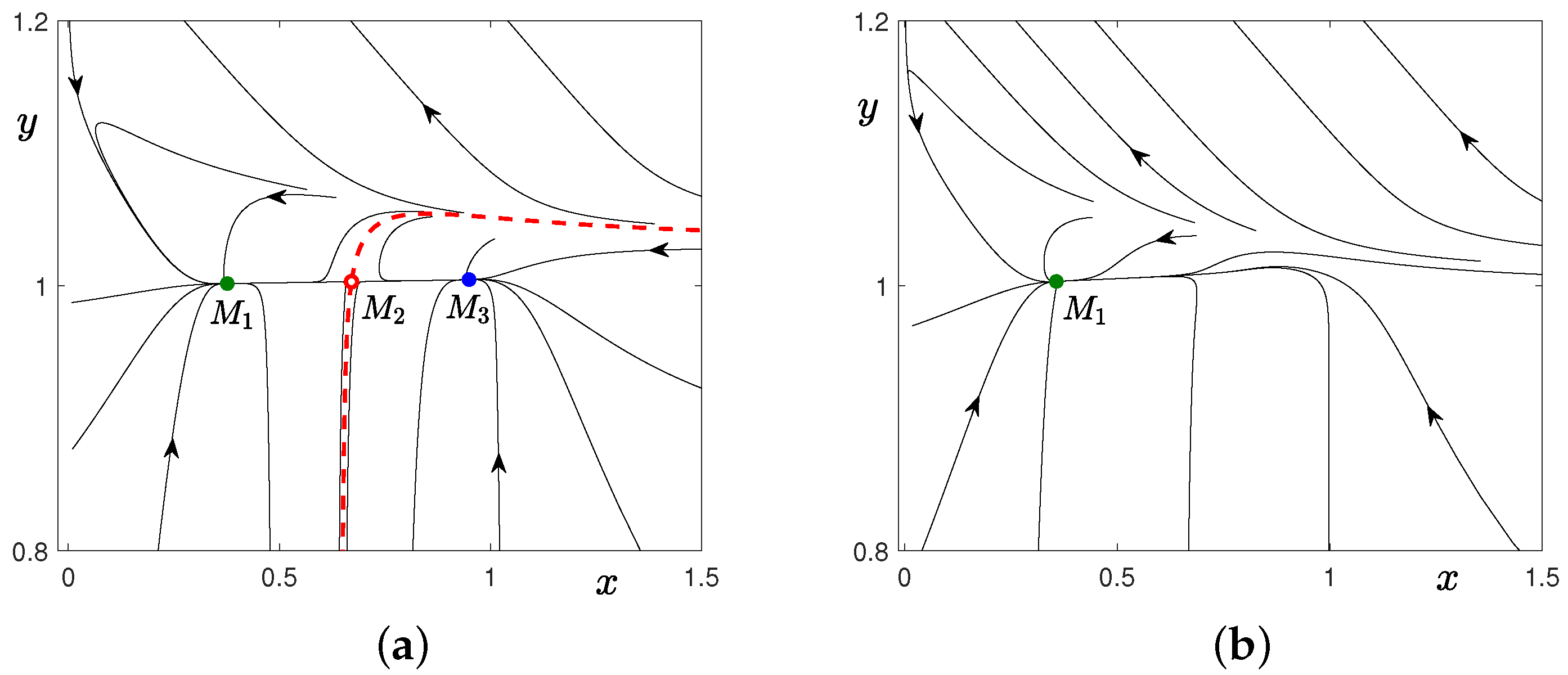
In Figure 2, we show phase portraits of the model (1) for D = 0.02 (Figure 2a) and D = 0.04 (Figure 2b). In Figure 2a, one can observe a coexistence of two stable nodes M 1 = ( 0.376486 , 1.00154 ) (filled green circle) and M 3 = ( 0.949131 , 1.00457 ) (filled blue circle). The stable manifold (dashed red line) of the saddle M 2 = ( 0.6708 , 1.00296 ) (empty red circle) creates the boundary between the basins of attraction of the two stable equilibria M 1 and M 3 .
In this case, a bistable scenario occurs in model (1). Depending on the initial condition, a solution can converge to one equilibrium state or the other. It should be mentioned that the equilibrium regimes M 1 and M 3 have almost the same temperature, but the concentration differs twice. Figure 2b exemplifies the monostable regime with only one equilibrium M 1 = ( 0.356612 , 1.00318 ) (filled green circle). This means that all solutions converge to only one state with a lower value of concentration.
In the following section, we consider a more complex bifurcation scenario.

2.2. Case 2: k 2 = 1 , γ = 75

In this case, the dynamical behavior of model (1) differs from the previous case and appears to be more complicated. There are also only up to three equilibria, but the stable equilibria that exist reflect the dynamics not only for different values of concentration, but also for different temperature levels. An additional complication is related to the emerging new bifurcation scenario. For this case, all bifurcation values of the parameter D are presented below:
D 1 = 0.01176245 D 2 = 0.01178143 D 3 = 0.01211245 D 4 = 0.01586245
D 5 = 0.0243 D 6 = 0.03262665 D 7 = 0.033195 D 8 = 0.0335 .
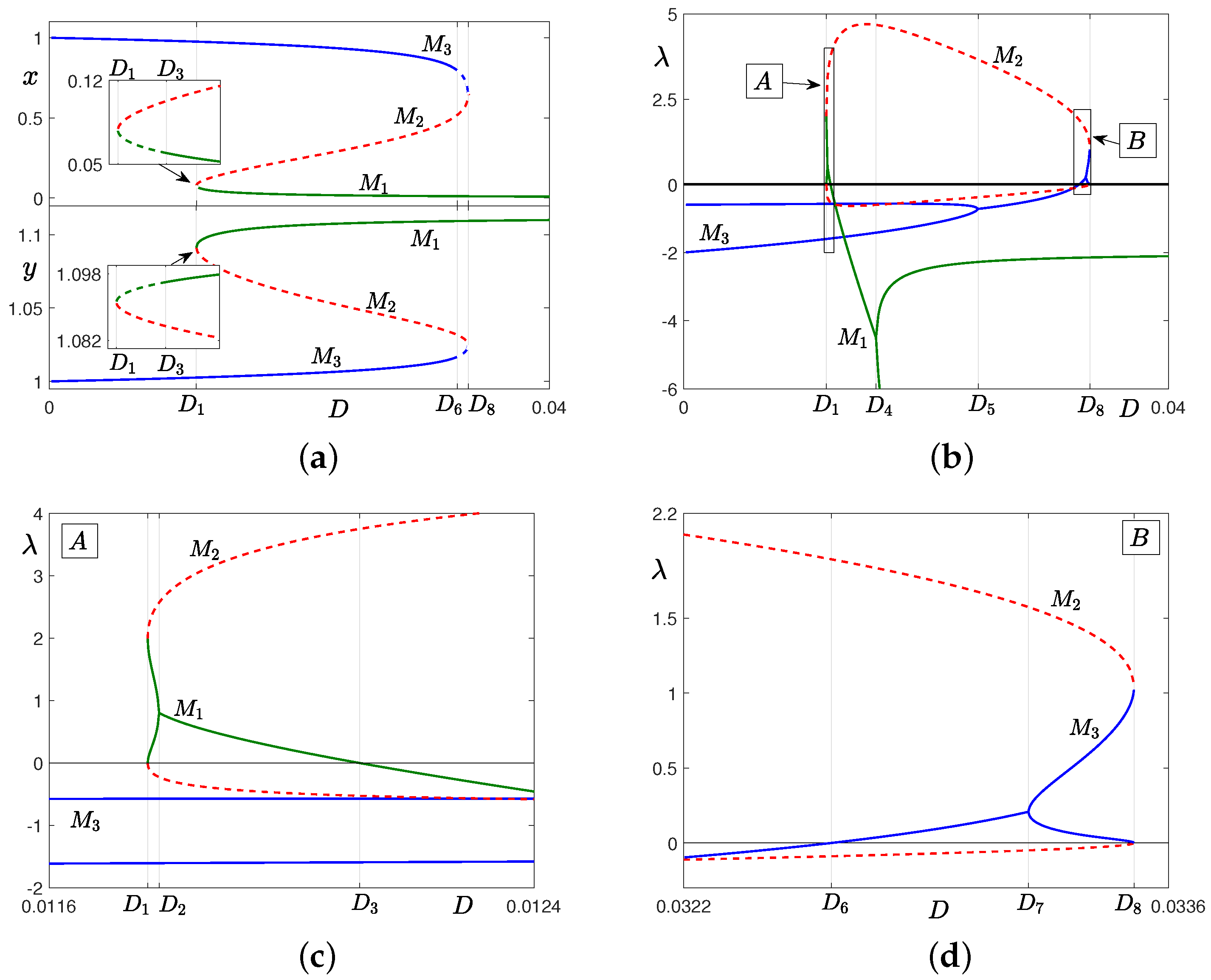
Figure 3 shows the bifurcation diagram and Lyapunov exponents of the equilibria of model (1) with k 2 = 1 , γ = 75 and changing parameter D. In the interval D ( 0 , D 1 ) , there is only one stable equilibrium M 3 (blue). At the bifurcation point D 1 , a saddle-node bifurcation occurs, which means that two equilibria M 1 (green) and M 2 (red) appear. Here, the Lyapunov exponents presented in Figure 3c provide more information.
First, at D = D 1 , the equilibrium M 1 is born as an unstable node: both Lyapunov exponents are real and positive. At D = D 2 , the Lyapunov exponents for M 1 become complex and the real part stays positive up to D = D 3 , so M 1 is an unstable focus. At D = D 3 , the real part becomes negative and remains so until the Lyapunov exponents become real again at D = D 4 , i.e., M 1 is a stable focus (see Figure 3b). For D > D 4 , Lyapunov exponents are real and negative, so M 1 is a stable node. At the same time, the Lyapunov exponents for the equilibrium M 2 have different signs in the parameter interval D 1 < D < D 8 , so M 2 is a saddle.
As for M 3 , this equilibrium is a stable node in the interval 0 < D < D 5 , where both its Lyapunov exponents are real and negative (see Figure 3b). At D = D 5 , the Lyapunov exponents become complex and the real part stays negative up to D = D 6 , so M 3 is a stable focus. At D = D 6 , the real part becomes positive and remains so until the Lyapunov exponents become real again at D = D 7 , i.e., M 3 is an unstable focus (see Figure 3d). In the interval D 7 < D < D 8 , the Lyapunov exponents are both real and positive, so M 3 is an unstable node. At the bifurcation value D 8 , a saddle-node bifurcation occurs, which means that the two equilibria M 2 and M 3 collide and disappear. Furthermore, for D > D 8 , only one stable equilibrium M 1 exists.
Thus, in this case, model (1) demonstrates bistable behavior in the interval D 3 < D < D 6 . Although in the intervals D 1 < D < D 3 and D 6 < D < D 8 there are three equilibria, there is only attracting one.
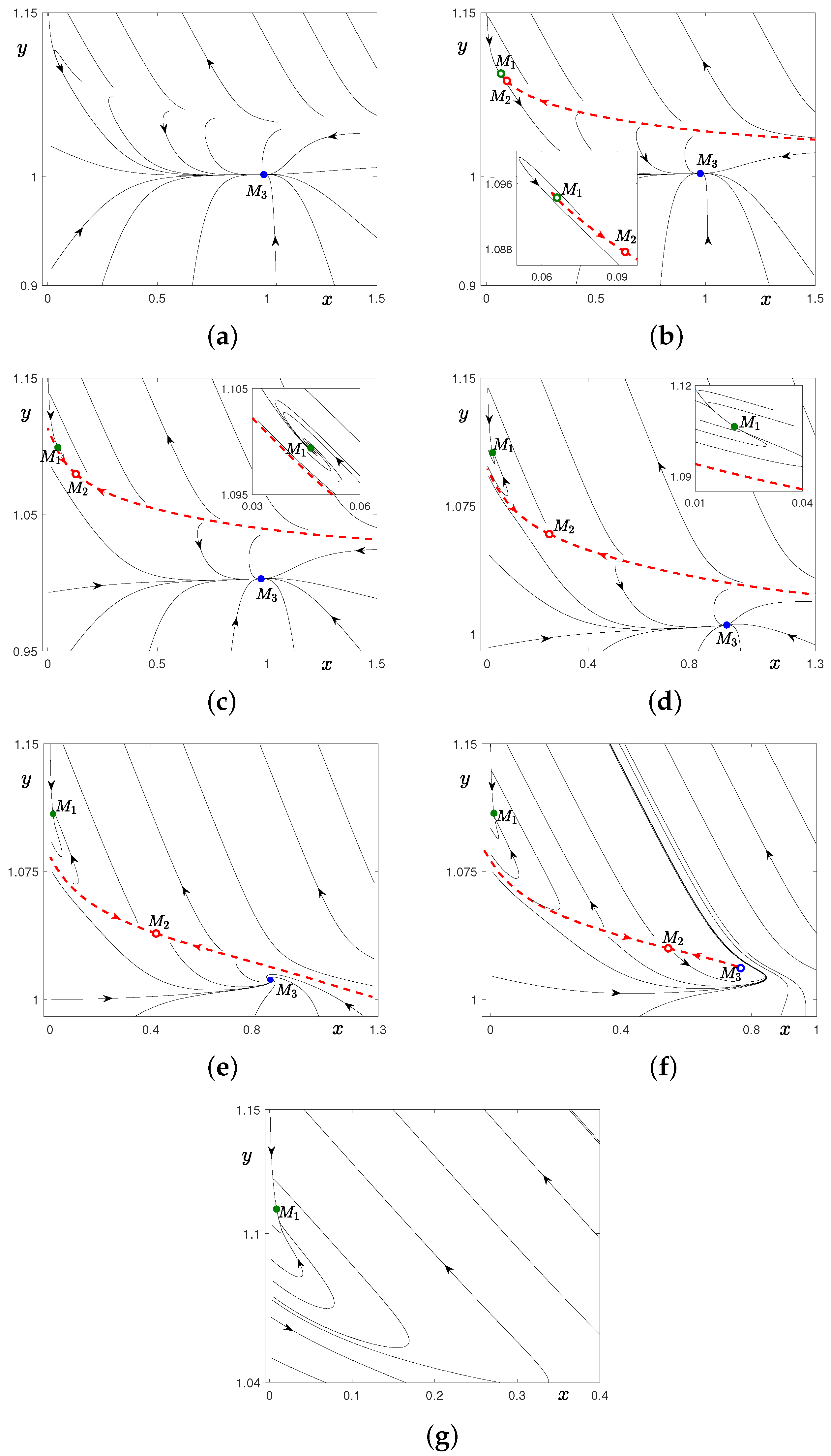
In Figure 4, we show the phase portraits of model (1) for different parameter zones. Figure 4a shows the dynamic regime for D = 0.008 with only one equilibrium M 3 = ( 0.984734 , 1.00167 ) (filled blue circle); this is a stable node. All trajectories converge to M 3 , which corresponds the attractive state with the higher concentration and lower temperature. It is worth noting that there are different types of transient process at play: one type of transient is formed by solutions converging immediately to equilibrium, the other first makes an ascent at the temperature and then with lower concentration converge to the equilibrium. This convergence behavior we observe while M 3 exists.
In Figure 4b for D = 0.0119 , a phase portrait with three equilibria is plotted. Here, M 1 = ( 0.066023 , 1.09427 ) (empty green circle) is an unstable focus, M 2 = ( 0.0931766 , 1.08765 ) (empty red circle) is a saddle, and M 3 = ( 0.975423 , 1.00265 ) (filled blue circle) is a stable node. The stable manifold (dashed red line) of the saddle M 2 creates a boundary between the two types of transients mentioned above.
Figure 4c exemplifies a coexistence of two stable equilibria for D = 0.013 : M 1 = ( 0.0463086 , 1.09939 ) (stable focus, filled green circle) and M 3 = ( 0.972488 , 1.00296 ) (stable node, filled blue circle). The stable manifold (dashed red line) of the saddle M 2 = ( 0.128324 , 0.128324 ) (empty red circle) is a separatrix between the basins of attraction of the two stable equilibria M 1 and M 3 . So, in this case, model (2) is bistable. Depending on the initial condition, the solution can converge to one equilibrium state or the other: one with a lower temperature and higher concentration, the other with a higher temperature and lower concentration.
In Figure 4d for D = 0.02 , a coexistence of two stable nodes, M 1 = ( 0.0209389 , 1.10638 ) (filled green circle) and M 3 = ( 0.948999 , 1.00527 ) (filled blue circle), and the saddle M 2 = ( 0.246123 , 1.05858 ) (empty red circle) is presented. The dynamical behavior is similar to one shown in Figure 4c with the difference being in the asymptotic behavior of M 1 (node instead of focus).
Figure 4e shows another slightly different scenario for D = 0.03 of the coexistence of two stable equilibria, M 1 = ( 0.0122653 , 1.10888 ) (filled green circle) and M 3 = ( 0.873089 , 1.01164 ) (filled blue circle), and the saddle M 2 = ( 0.420613 , 1.03871 ) (empty red circle). Here, M 1 is a stable node while M 3 is a stable focus.
In Figure 4f for D = 0.033 , the equilibrium M 1 = ( 0.0109274 , 1.10927 ) (filled green circle) is a stable node, M 2 = ( 0.545091 , 0.545091 ) (empty red circle) is a saddle, and M 3 = ( 0.766769 , 1.01842 ) (empty blue circle) is an unstable focus. By the red dashed line, we show the stable manifold of the saddle M 2 that creates a boundary between two types of the transient behavior.
Figure 4g shows the dynamic regime for D = 0.04 with only one equilibrium M 1 = ( 0.00871817 , 1.10991 ) (filled green circle); this is a stable node. This means that all solutions of the system (1) converge to only one state with lower value of concentration and with higher temperatures.
To summarize, this thermo-kinetic model exhibits a diversity of complex dynamic regimes even in the deterministic case. In the next section, we will consider additional effects caused by random disturbances.

3. Stochastic Model

Let us consider a stochastic version of the thermo-kinetic model with multiplicative random disturbances:
x ˙ = k 1 ( 1 x ) x f ( y ) k 2 x ( 1 x ) 2 + ε x ξ ( t ) , y ˙ = β x f ( y ) + s ( 1 y ) .
Here, ξ ( t ) is a scalar white Gaussian noise with parameters E ξ ( t ) = 0 , E ξ ( t ) ξ ( τ ) = δ ( t τ ) , and ε is the noise intensity. In stochastic simulation of random solutions of the system (3), we use the Euler–Maruyama scheme with the time step 0.001.

3.1. Stochastic Effects in the Case 1 with k 2 = 2.5 , γ = 55

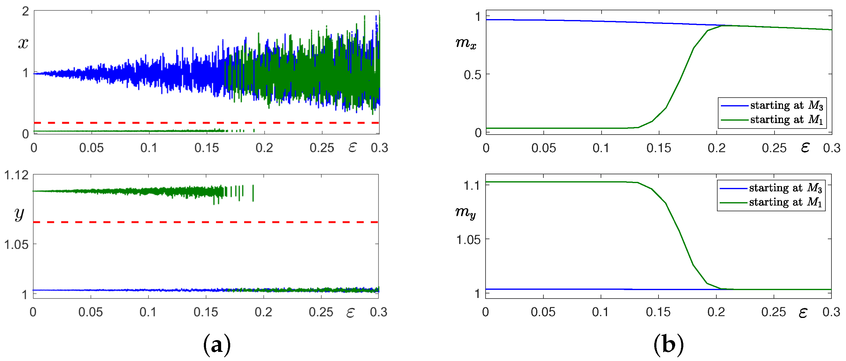
First, we consider the bistability parameter range 0 < D < D 1 = 0.03323 where deterministic system (1) has two stable equilibria (see Section 2.1). For D = 0.02 , Figure 5a shows the x- and y-coordinates of random solutions of system (3) starting at M 1 (green) and M 3 (blue) versus noise intensity. Here and further, we use the following colors designation: if the trajectory starts at the equilibrium M 1 ( M 3 ) then random states (Figure 5a and Figure 6a), mean values (Figure 5b and Figure 6b), time series (Figure 7 and Figure 8), and probability (Figure 9 and Figure 10) are plotted in green (blue). First, the dispersion of random states around both equilibria increases. For ε 0.05 , solutions starting at M 3 (blue) begin to transit to M 1 . For ε > 0.1 , a reverse transition from the equilibrium M 1 to the basin of M 3 begins to be observed. The results of the statistical analysis of these stochastic transformations are shown in Figure 5b in terms of mean values m x , m y versus noise intensity. For noise intensity ε < 0.04 , two mean values differ. With a further increase in ε , the mean values of random solutions starting at M 3 (blue) rapidly decrease and merge with the mean values of random solutions starting at M 1 (green). After such a merging, the mean values slowly increase.
In order to give a parametric description of the observed noise-induced transitions, we will use the stochastic sensitivity function technique [27,28,29,30,31]. This technique was introduced for constructive approximation of the probabilistic distribution of random states in the neighborhood of the deterministic attractor. The stochastic sensitivity function technique was first elaborated for continuous-time systems and now covers cases of such attractors as equilibria, limit cycles, and tori [27,30,31,34]. Moreover, for discrete-time systems, the theory of stochastic sensitivity was elaborated also for closed invariant curves [35] and chaotic attractors [36]. This theory is effectively used in the stochastic analysis of nonlinear dynamic models in various fields of science (see, e.g., [33,37,38,39]), and also in control problems [40,41].
Geometrically, the stochastic sensitivity function technique can be applied in the form of confidence domains [29,32]. Such domains calculated by this technique allow one to get a clear spatial description of the random states’ dispersion near the deterministic attractor.
For the stable equilibrium M ( x ¯ , y ¯ ) of the two-dimensional stochastic system, a dispersion of random states can be approximated by a confidence ellipse
z 1 2 μ 1 + z 2 2 μ 2 = 2 ε 2 ln ( 1 P ) ,
where parameters μ 1 > μ 2 are eigenvalues of the stochastic sensitivity matrix W, variables z 1 and z 2 are coordinates of this ellipse in the basis of orthonormal eigenvectors u 1 , u 2 of the matrix W, the parameter ε is the noise intensity, and P stands for the fiducial probability.
So, when constructing the confidence ellipse, one has to calculate the stochastic sensitivity matrix W. This matrix is a unique solution of the algebraic Equation [28]
J W + W J + G = 0 ,
where J is a Jacobi matrix of the original deterministic system at the equilibrium point M ( x ¯ , y ¯ ) and the matrix G reflects an influence of the random disturbances. For the system (3), we have
J ( x , y ) = k 1 D e γ ( 1 1 y ) k 2 ( 1 4 x + 3 x 2 ) γ D x y 2 e γ ( 1 1 y ) β D e γ ( 1 1 y ) β γ D x y 2 e γ ( 1 1 y ) s ,
G ( x ) = diag [ x 2 , 0 ] .
The stochastic sensitivity matrix W allows one to approximate the covariance matrix of solutions ( x ε ( t ) , y ε ( t ) ) of the stochastic system near the equilibrium M ( x ¯ , y ¯ ) :
c o v ( x ε ( t ) , y ε ( t ) ) ε 2 W .
Spatial peculiarities of the dispersion of random solutions ( x ε ( t ) , y ε ( t ) ) near the equilibrium M ( x ¯ , y ¯ ) are reflected by eigenvalues and eigenvectors of the matrix W. Indeed, eigenvalues μ 1 , μ 2 of the stochastic sensitivity matrix W define the eccentricity and size of the confidence ellipse in directions of eigenvectors u 1 , u 2 . Note that the extent of the ellipse is proportional to the noise intensity ε .
So, the spectral characteristics of the matrix W make it possible to obtain an approximation of the probability density near the equilibrium in the Gaussian form:
ρ ( z 1 , z 2 ) = K e z 1 2 2 μ 1 ε 2 z 2 2 2 μ 2 ε 2 .
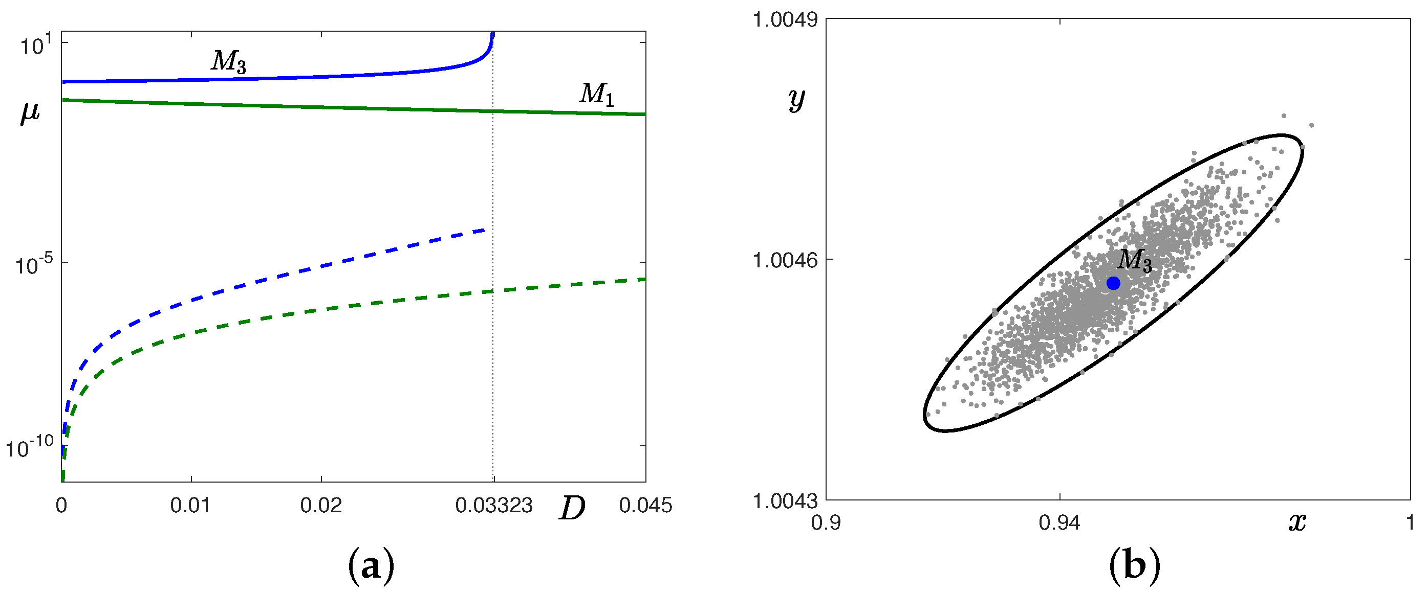
Consider how this stochastic sensitivity technique can be used in analysis of the noise-induced transitions in system (3). In Figure 11a, eigenvalues μ 1 (solid) and μ 2 (dashed) ( μ 1 > μ 2 > 0 ) of the stochastic sensitivity matrix of equilibria M 1 (green) and M 3 (blue) are plotted versus parameter D. Note that both eigenvalues for M 3 are bigger then the eigenvalues for M 1 . This means that the dispersion of stochastic states around the equilibrium M 3 would be wider. The largest eigenvalue μ 1 of the stochastic sensitivity matrix for the equilibrium M 3 increases sharply when parameter D approaches the bifurcation value D 1 , while the value of μ 1 for the equilibrium M 1 slightly decreases with an increase in parameter D. Figure 11b shows an example of the confidence ellipse around the equilibrium M 3 for D = 0.02 and noise intensity ε = 0.01 constructed using the stochastic sensitivity matrix. Note that dispersion of random states (grey) is well approximated by this ellipse.
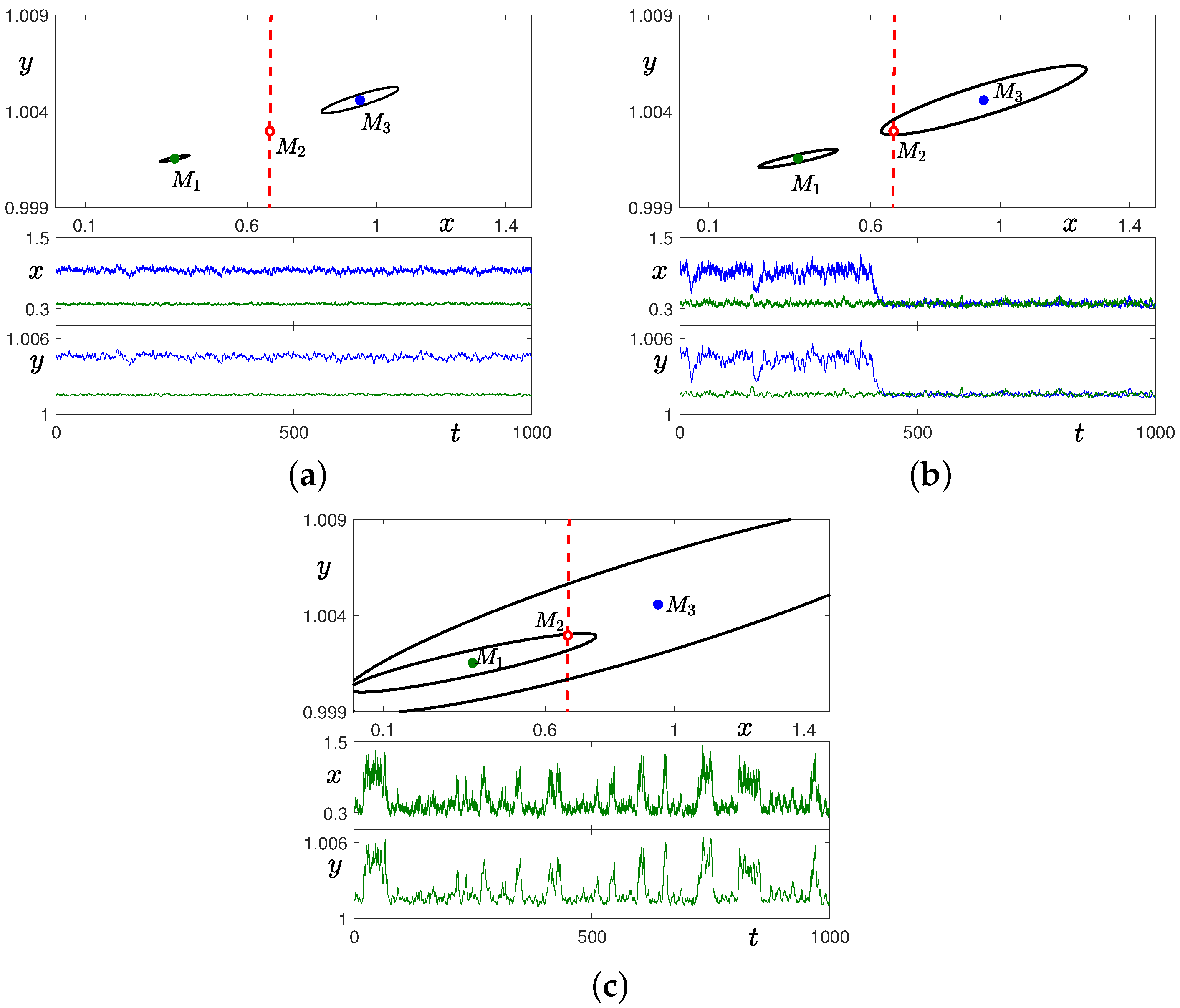
The relative position of the confidence ellipses and the boundary of the basin of attraction of a deterministic attractor makes it possible to describe noise-induced transitions. Figure 7 demonstrates an application of this method. For the noise intensity ε = 0.03 in Figure 7a (top), confidence ellipses (black) for both equilibria lie far from the separatrix (red dashed line) between the basins of attraction of the equilibria M 1 and M 3 . This means that random states are localized near M 1 or M 3 , and transitions do not occur. This behavior is shown by the time series in Figure 7a (bottom).
In Figure 7b (top), for ε = 0.08 , one of the confidence ellipses, related to equilibrium M 3 , crosses the boundary of the basins of attraction. This indicates the occurrence of a noise-induced transition from M 3 to M 1 , which is shown in the time series below. The situation where both ellipses cross the separatrix is presented for ε = 0.25 in Figure 7c (top). In this case, we observe noise-induced two-way transitions between two equilibria M 1 M 3 , which are shown in the time series in Figure 7c (bottom).
In the case under consideration, the stochastic system (3) demonstrates two-stage noise-induced transitions between two modes corresponding to states with different value of concentration x and almost equal values of temperature y. The first stage is the one-way transition from a larger value of the concentration to a smaller value ( M 3 M 1 ), and the second stage (stochastic trigger) is intermittent behavior between these two concentration values ( M 1 M 3 ).
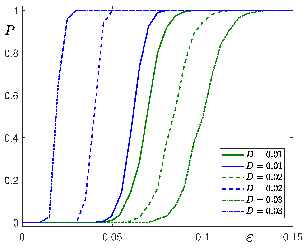
The results of the statistical analysis in terms of the probability P of transitions are given in Figure 9 versus noise intensity ε for various values of the parameter D (the color matches the equilibrium from which we observe the transition). Here, we use the x-coordinate of the equilibrium M 2 as a threshold value. First, transitions from equilibria M 1 occur for higher levels of noise intensity ε . Second, for both equilibria, the following remark holds: the larger the value of D, the higher the required noise intensity for transitions.

3.2. Stochastic Effects in the Case 2 with k 2 = 1 , γ = 75

Now, we consider stochastic system (3) with k 2 = 1 , γ = 75 in the bistable parameter region D 3 < D < D 6 where the initial deterministic model exhibits a coexistence of two stable equilibria M 1 and M 3 (see Figure 3a). Figure 6a shows the x- and y-coordinates of the random states of the stochastic solutions starting at M 1 (green) and M 3 (blue) versus noise intensity for D = 0.015 . First, as the noise increases, the dispersion of random states around both equilibria increases as well. For noise intensity ε 0.15 , solutions starting at M 1 (green) demonstrate transitions to M 3 . In Figure 6b, these transitions are shown in terms of the mean values m x , m y of the stochastic states. For noise intensity ε < 0.15 , the two mean values differ, but with further increases in ε , the mean values of the random states of the stochastic solutions starting at M 1 (green) rapidly increase and merge with the mean values for M 3 (blue). After this merging, both mean values slowly decrease. It is worth noting that in this case, only one-way noise-induced transitions M 1 M 3 are observed.
As in the previous case, when studying the noise-induced transitions, we will use the stochastic sensitivity function and method of confidence domains. Eigenvalues of the stochastic sensitivity matrix for equilibria M 1 (green) and M 3 (blue) are presented in Figure 12. For M 3 , the largest eigenvalue is bigger than the eigenvalues for M 1 . This is almost a constant for most of the interval 0 < D < D 6 and only increases for D > 0.032 . Eigenvalues for the equilibrium M 1 decrease as the parameter D moves to the right from D 3 .
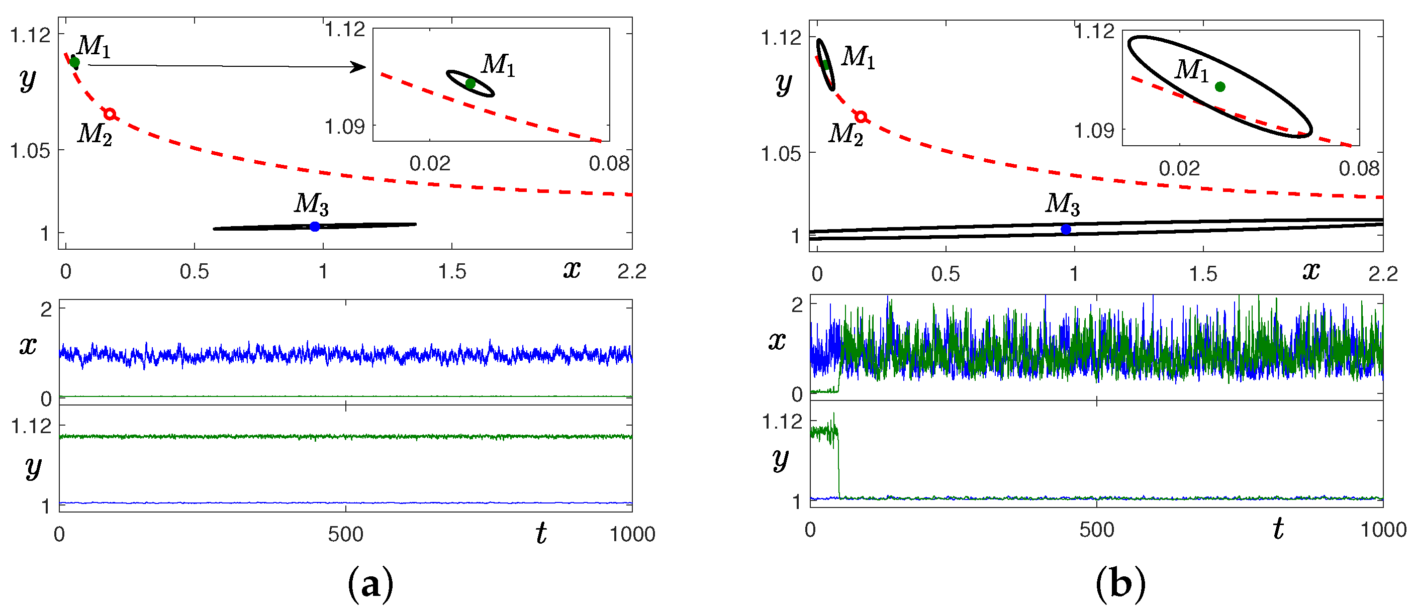
Despite the fact that the sensitivity of the equilibrium M 3 is higher than sensitivity of the equilibrium M 1 , and the spread of random states is larger around the equilibrium M 3 , no transitions from M 3 to M 1 are detected. On the contrary, the transition from M 1 to M 3 occurs (see Figure 6). This fact can be explained by the following: the equilibrium M 1 is much closer to the separatrix (red dashed line) than the equilibrium M 3 (see Figure 8). In the top panels of Figure 8, we show confidence ellipses (black curves) around both equilibria for two values of the noise intensity. For ε = 0.1 (Figure 8a), both confidence ellipses do not intersect the separatrix. This means that random states are localized near equilibria M 1 or M 3 , and transitions do not occur. This behavior is shown by the time series in Figure 8a, bottom. For ε = 0.4 (Figure 8b), one of the confidence ellipses, related to the equilibrium M 1 , crosses the boundary of the basins of attraction. This indicates the occurrence of a noise-induced transition from M 1 to M 3 . This transition is shown in the time series below.
So, in case 2, in contrast to case 1 described in Section 3.1, stochastic system (3) demonstrates only one-stage noise-induced transitions, namely from the mode with a lower value of concentration x and a larger temperature y to the mode with a larger value of concentration x and a smaller temperature y ( M 1 M 3 ).
Details of the statistical analysis of these stochastic transformations are shown in Figure 10, where the probability P of transitions M 1 M 3 is plotted versus noise intensity ε for various values of the parameter D. Here, as before, we use the x-coordinate of the equilibrium M 2 as a threshold value. The larger the value of D, the higher the required noise intensity for transitions.

4. Conclusions

This paper is devoted to the problem of the mathematical modeling and computer simulation of complex nonlinear processes in the thermo-kinetics of autocatalysis. In our study, we considered a mathematical model of the dynamic interaction of reagent concentration and temperature. Parametric zones of bistability with the coexistence of two equilibrium regimes of thermo-kinetics were investigated. It was shown how random disturbances can deform deterministic dynamic regimes. When studying these noise-induced transformations, we applied the methods of direct numerical simulation with the subsequent statistical processing as well as the analytical stochastic sensitivity technique and apparatus of confidence domains. Two variants of bistability with different scenarios of stochastic transformations are studied and compared. The main result of this paper is a detailed analysis of noise-induced shifts in the probabilistic distributions of random states and probability of transitions from one equilibrium mode to another. For understanding underlying mechanisms of such transition, a key role of the mutual arrangement of basins of attractors, separatrices, and confidence ellipses is demonstrated. It is worth noting that this approach can be applied to the analysis of more complex stochastic models in various fields of science. The results presented in the paper shed light on the probabilistic mechanisms of the generation of complex oscillatory modes that appear in autocatalysis.

Author Contributions

Conceptualization, I.B. and L.R.; methodology, L.R.; software, T.P. and M.P.; validation, T.P., M.P. and I.B.; formal analysis, T.P.; investigation, T.P., M.P. and I.B.; resources, T.P.; data curation, M.P.; writing—original draft preparation, T.P. and I.B.; writing—review and editing, T.P. and I.B.; visualization, M.P.; supervision, L.R.; project administration, L.R.; funding acquisition, L.R. All authors have read and agreed to the published version of the manuscript.

Funding

This research was funded by the Ministry of Science and Higher Education of the Russian Federation (Ural Federal University Program of Development within the Priority-2030 Program).

Data Availability Statement

The data presented in this study are available on request from the corresponding author.

Conflicts of Interest

The authors declare no conflict of interest.

References

  1. Schmidt, L.D. The Engineering of Chemical Reactions; Oxford University Press: New York, NY, USA, 1998. [Google Scholar]
  2. Davis, M.E. Fundamentals of Chemical Reaction Engineering; McGraw-Hill: Boston, MA, USA, 2003. [Google Scholar]
  3. Bykov, V.I.; Tsybenova, S.B.; Yablonsky, G. Chemical Complexity via Simple Models; De Gruyter: Berlin, Germany, 2018. [Google Scholar]
  4. Uppal, A.; Ray, W.H.; Poore, A.B. The classification of the dynamic behavior of continuous stirred tank reactors—Influence of reactor resident time. Chem. Eng. Sci. 1976, 31, 205–214. [Google Scholar] [CrossRef]
  5. Kawczyński, A.L.; Gorecki, J. Molecular dynamics simulations of sustained oscillations in a thermochemical system. J. Phys. Chem. 1992, 96, 1060–1067. [Google Scholar] [CrossRef]
  6. Kawczyński, A.L.; Nowakowski, B. Master equation simulations of a model of a thermochemical system. Phys. Rev. E 2003, 68, 036218. [Google Scholar] [CrossRef] [PubMed]
  7. Bashkirtseva, I.; Ivanenko, G.; Mordovskikh, D.; Ryashko, L. Canards oscillations, noise-induced splitting of cycles and transition to chaos in thermochemical kinetics. Mathematics 2023, 11, 1918. [Google Scholar] [CrossRef]
  8. Shilnikov, L.P.; Shilnikov, A.L.; Turaev, D.V.; Chua, L.O. Methods of Qualitative Theory in Nonlinear Dynamics; World Scientific: Singapore, 1998; p. 416. [Google Scholar]
  9. Guckenheimer, J.; Holmes, P. Nonlinear Oscillations, Dynamical Systems, and Bifurcations of Vector Fields; Springer: Berlin/Heidelberg, Germany, 1983; p. 462. [Google Scholar]
  10. Kuznetsov, Y.A. Elements of Applied Bifurcation Theory; Springer: Berlin/Heidelberg, Germany, 1998. [Google Scholar]
  11. Kloeden, P.E.; Platen, E.; Schurz, H. Numerical Solution of SDE Through Computer Experiments; Springer: Berlin/Heidelberg, Germany, 2002; p. 294. [Google Scholar]
  12. Gautschi, W. Numerical Analysis; Springer: Berlin/Heidelberg, Germany, 2011. [Google Scholar]
  13. Awrejcewicz, J. Numerical Simulations of Physical and Engineering Processes; InTech: Rijeka, Croatia, 2011; p. 614. [Google Scholar]
  14. Butcher, J.C. Numerical Methods for Ordinary Differential Equations; Wiley: Chichester, UK, 2016; p. 544. [Google Scholar]
  15. Milstein, G.N.; Tretyakov, M.V. Stochastic Numerics for Mathematical Physics; Springer: Berlin/Heidelberg, Germany, 2021; p. 736. [Google Scholar]
  16. Bykov, V.; Tsybenova, S. A model of thermokinetic oscillations on the surface of a catalyst. Russ. J. Phys. Chem. A 2003, 77, 1402–1405. [Google Scholar]
  17. Tsybenova, S. The basic thermokinetic models. Phys.-Chem. Kinet. Gas Dyn. 2008, 6, 281. [Google Scholar]
  18. Bykov, V.; Tsybenova, S. A parametric analysis of the basic nonlinear models of the catalytic reactions. Math. Model. Nat. Phenom. 2015, 10, 68–83. [Google Scholar] [CrossRef]
  19. Horsthemke, W.; Lefever, R. Noise-Induced Transitions; Springer: Berlin/Heidelberg, Germany, 1984; p. 338. [Google Scholar]
  20. Anishchenko, V.S.; Astakhov, V.V.; Neiman, A.B.; Vadivasova, T.E.; Schimansky-Geier, L. Nonlinear Dynamics of Chaotic and Stochastic Systems. Tutorial and Modern Development; Springer: Berlin/Heidelberg, Germany, 2007; p. 535. [Google Scholar]
  21. Arnold, L. Random Dynamical Systems; Springer: Berlin/Heidelberg, Germany, 1998; p. 600. [Google Scholar]
  22. Lindner, B.; Garcia-Ojalvo, J.; Neiman, A.; Schimansky-Geier, L. Effects of noise in excitable systems. Phys. Rep. 2004, 392, 321–424. [Google Scholar] [CrossRef]
  23. McDonnell, M.D.; Stocks, N.G.; Pearce, C.E.M.; Abbott, D. Stochastic Resonance: From Suprathreshold Stochastic Resonance to Stochastic Signal Quantization; Cambridge University Press: Cambridge, UK, 2008; p. 446. [Google Scholar]
  24. Gardiner, C.W. Handbook of Stochastic Methods for Physics, Chemistry and the Natural Sciences; Springer: Berlin/Heidelberg, Germany, 1983. [Google Scholar]
  25. Freidlin, M.I.; Wentzell, A.D. Random Perturbations of Dynamical Systems; Springer: New York, NY, USA; Berlin, Germany, 1984. [Google Scholar]
  26. Mil’shtein, G.N.; Ryashko, L.B. A first approximation of the quasipotential in problems of the stability of systems with random non-degenerate perturbations. J. Appl. Math. Mech. 1995, 59, 47–56. [Google Scholar] [CrossRef]
  27. Bashkirtseva, I.; Ryashko, L. Stochastic sensitivity of 3D-cycles. Math. Comput. Simul. 2004, 66, 55–67. [Google Scholar] [CrossRef]
  28. Bashkirtseva, I.; Ryashko, L. Sensitivity and chaos control for the forced nonlinear oscillations. Chaos Solitons Fractals 2005, 26, 1437–1451. [Google Scholar] [CrossRef]
  29. Ryashko, L.; Bashkirtseva, I.; Gubkin, A.; Stikhin, P. Confidence tori in the analysis of stochastic 3D-cycles. Math. Comput. Simul. 2009, 80, 256–269. [Google Scholar] [CrossRef]
  30. Bashkirtseva, I.; Ryashko, L. Sensitivity analysis of stochastic attractors and noise-induced transitions for population model with Allee effect. Chaos 2011, 21, 047514. [Google Scholar] [CrossRef]
  31. Bashkirtseva, I. Stochastic sensitivity analysis: Theory and numerical algorithms. IOP Conf. Ser. Mater. Sci. Eng. 2017, 192, 012024. [Google Scholar] [CrossRef]
  32. Chen, J.; Zhang, T.; Zhou, Y. Stochastic sensitivity and dynamical complexity of newsvendor models subject to trade credit. Math. Comput. Simul. 2021, 181, 471–486. [Google Scholar] [CrossRef]
  33. Bashkirtseva, I.; Perevalova, T. Analysis of stochastic bifurcations in the eco-epidemiological oscillatory model with weak Allee effect. Int. J. Bifurc. Chaos 2022, 32, 2250124. [Google Scholar] [CrossRef]
  34. Bashkirtseva, I.; Ryashko, L. Sensitivity analysis of stochastically forced quasiperiodic self-oscillations. Electron. J. Differ. Equ. 2016, 2016, 1–12. [Google Scholar]
  35. Bashkirtseva, I.; Ryashko, L. Stochastic sensitivity of the closed invariant curves for discrete-time systems. Phys. A 2014, 410, 236–243. [Google Scholar] [CrossRef]
  36. Bashkirtseva, I.; Ryashko, L. Stochastic sensitivity of regular and multi-band chaotic attractors in discrete systems with parametric noise. Phys. Lett. A 2017, 381, 3203–3210. [Google Scholar] [CrossRef]
  37. Alexandrov, D.V.; Bashkirtseva, I.A.; Crucifix, M.; Ryashko, L.B. Nonlinear climate dynamics: From deterministic behaviour to stochastic excitability and chaos. Phys. Rep. 2021, 902, 1–60. [Google Scholar] [CrossRef]
  38. Slepukhina, E.; Bashkirtseva, I.; Ryashko, L.; Kügler, P. Stochastic mixed-mode oscillations in the canards region of a cardiac action potential model. Chaos Solitons Fractals 2022, 164, 112640. [Google Scholar] [CrossRef]
  39. Bashkirtseva, I.; Chukhareva, A.; Ryashko, L. Stochastic dynamics of nonlinear tumor–immune system with chemotherapy. Physica A 2023, 622, 128835. [Google Scholar] [CrossRef]
  40. Bashkirtseva, I. Method of stochastic sensitivity synthesis in a stabilisation problem for nonlinear discrete systems with incomplete information. Int. J. Control 2017, 90, 1652–1663. [Google Scholar] [CrossRef]
  41. Bashkirtseva, I.; Ryashko, L.; Chen, G. Stochastic sensitivity synthesis in nonlinear systems with incomplete information. J. Frankl. Inst. 2020, 357, 5187–5198. [Google Scholar] [CrossRef]
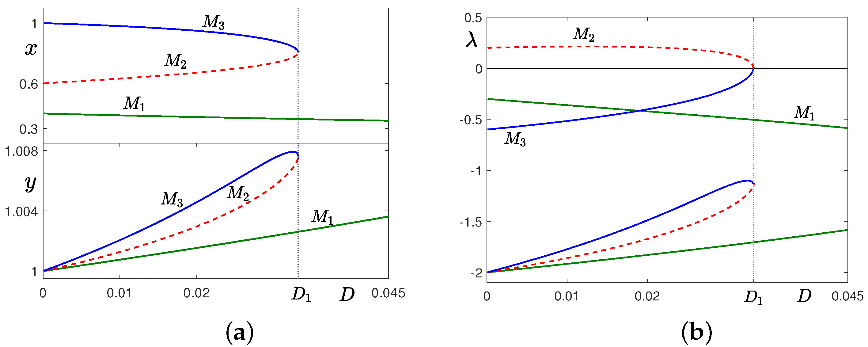
Figure 1. System (1) with k 2 = 2.5 , γ = 55 : (a) coordinates, x (top) and y (bottom), of the equilibria M 1 (green), M 2 (red dashed), and M 3 (blue). Here, M 1 and M 3 are stable nodes and M 2 is a saddle. In (b), the Lyapunov exponents are shown by the corresponding colors.
Mathematics 11 04302 g001
Figure 2. Phase portraits of the system (1) with k 2 = 2.5 , γ = 55 for: (a) D = 0.02 and (b) D = 0.04 . Here, M 1 (filled green circle) and M 3 (filled blue circle) are stable nodes, and M 2 (empty red circle) is a saddle. Here, the separatrix shown by the red dashed line is the stable manifold of the saddle M 2 . Arrows show evolution over time.
Mathematics 11 04302 g002
Figure 3. System (1) with k 2 = 1 , γ = 75 : (a) coordinates, x (top) and y (bottom), of the equilibria M 1 (green), M 2 (red dashed), and M 3 (blue). In (bd), the Lyapunov exponents are shown by the corresponding colors.
Mathematics 11 04302 g003
Figure 4. Phase portraits of model (1) with k 2 = 1 , γ = 75 for: (a) D = 0.008 , (b) D = 0.0119 , (c) D = 0.013 , (d) D = 0.02 , (e) D = 0.03 , (f) D = 0.033 , and (g) D = 0.04 . The equilibria M 1 , M 2 , and M 3 are shown by green, red, and blue, respectively. Here, the separatrix shown by a red dashed line is the stable manifold of the saddle M 2 . Arrows show evolution over time.
Mathematics 11 04302 g004
Figure 5. Stochastic system (3) with k 2 = 2.5 , γ = 55 , D = 0.02 : (a) random states of solutions starting at M 1 (green) and M 3 (blue); (b) corresponding mean values. Here, red dashed lines mark coordinates of the equilibrium M 2 .
Mathematics 11 04302 g005
Figure 6. Stochastic system (3) with k 2 = 1 , γ = 75 , D = 0.015 : (a) random states of solutions starting at M 1 (green) and M 3 (blue); (b) corresponding mean values. Here, red dashed lines mark coordinates of the equilibrium M 2 .
Mathematics 11 04302 g006
Figure 7. Noise-induced transitions in system (3) with k 2 = 2.5 , γ = 55 , D = 0.02 between equilibria M 1 (green circle) and M 3 (blue circle): (a) no transition for ε = 0.03 , (b) transition M 3 M 1 for ε = 0.08 , (c) transitions M 1 M 3 for ε = 0.25 . Here, red dashed lines mark the separatrices. In top panels, we show equilibria and confidence ellipses. In bottom panels, we show time series of solutions starting at M 1 / M 3 in green/blue.
Mathematics 11 04302 g007
Figure 8. Noise-induced transitions in stochastic system (3) with k 2 = 1 , γ = 75 , D = 0.015 : (a) no transition for ε = 0.1 , (b) transition from M 1 (green circle) to M 3 (blue circle) for ε = 0.4 . Here, red dashed lines mark the separatrices. In top panels, we show equilibria and confidence ellipses. In bottom panels, we show time series of solutions starting at M 1 / M 3 in green/blue.
Mathematics 11 04302 g008
Figure 9. Probability P ( ε ) of noise-induced transitions in system (3) with k 2 = 2.5 , γ = 55 for different values of the parameter D: M 3 M 1 (blue) and M 1 M 3 (green).
Mathematics 11 04302 g009
Figure 10. Probability of noise-induced transitions M 1 M 3 in stochastic system (3) with k 2 = 1 , γ = 75 .
Mathematics 11 04302 g010
Figure 11. Stochastic sensitivity of equilibria M 1 and M 3 in system (3) with k 2 = 2.5 , γ = 55 : (a) eigenvalues μ 1 (solid) and μ 2 (dashed) ( μ 1 > μ 2 > 0 ) of the stochastic sensitivity matrix W of equilibria M 1 (green) and M 3 (blue), (b) confidence ellipse (black) and stochastic states (grey) for the equilibrium M 3 (blue) with D = 0.02 and noise intensity ε = 0.01 .
Mathematics 11 04302 g011
Figure 12. Eigenvalues μ 1 (solid) and μ 2 (dashed) ( μ 1 > μ 2 > 0 ) of the stochastic sensitivity matrix of equilibria M 1 (green) and M 3 (blue) in stochastic system (3) with k 2 = 1 , γ = 75 .
Mathematics 11 04302 g012
Disclaimer/Publisher’s Note: The statements, opinions and data contained in all publications are solely those of the individual author(s) and contributor(s) and not of MDPI and/or the editor(s). MDPI and/or the editor(s) disclaim responsibility for any injury to people or property resulting from any ideas, methods, instructions or products referred to in the content.