
Normalization Method as a Potent Tool for Grasping Linear and Nonlinear Systems in Physics and Soil Mechanics

 ,
,  ,
,  ,
,  and
and 
Abstract
:1. Introduction
2. Normalization Technique
3. Illustrative Applications of the Normalization Technique
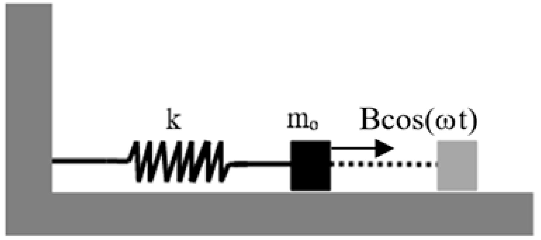
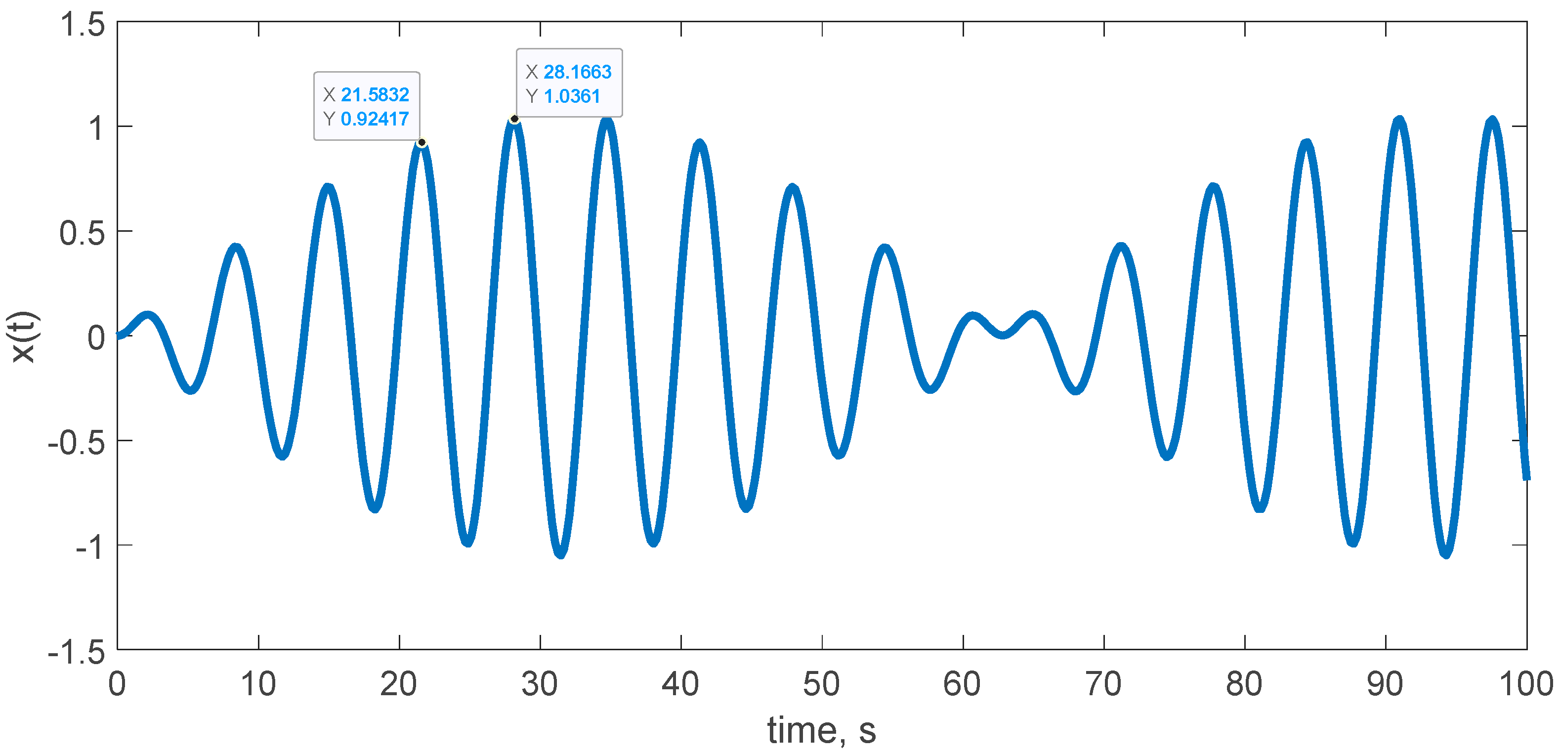
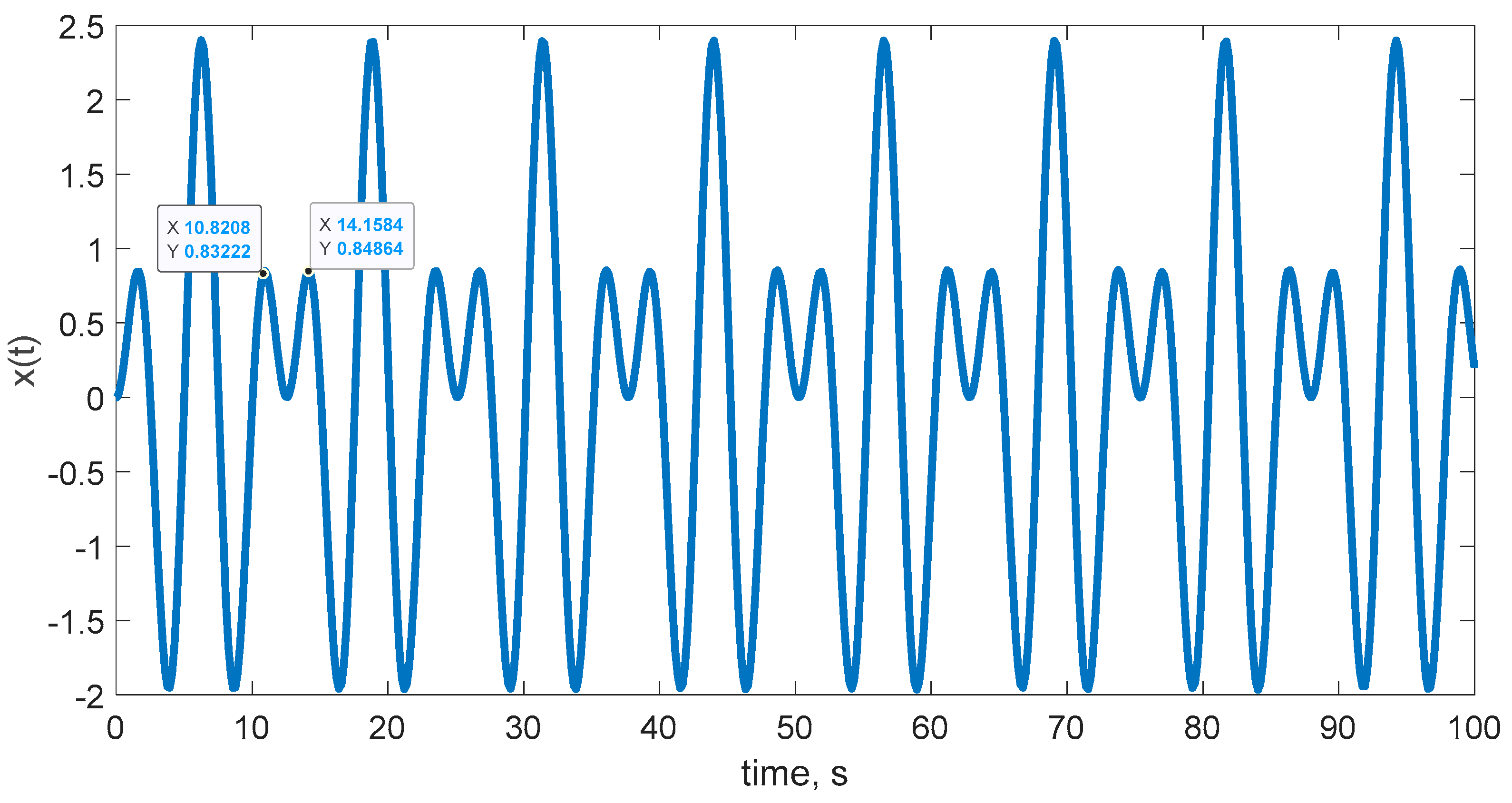
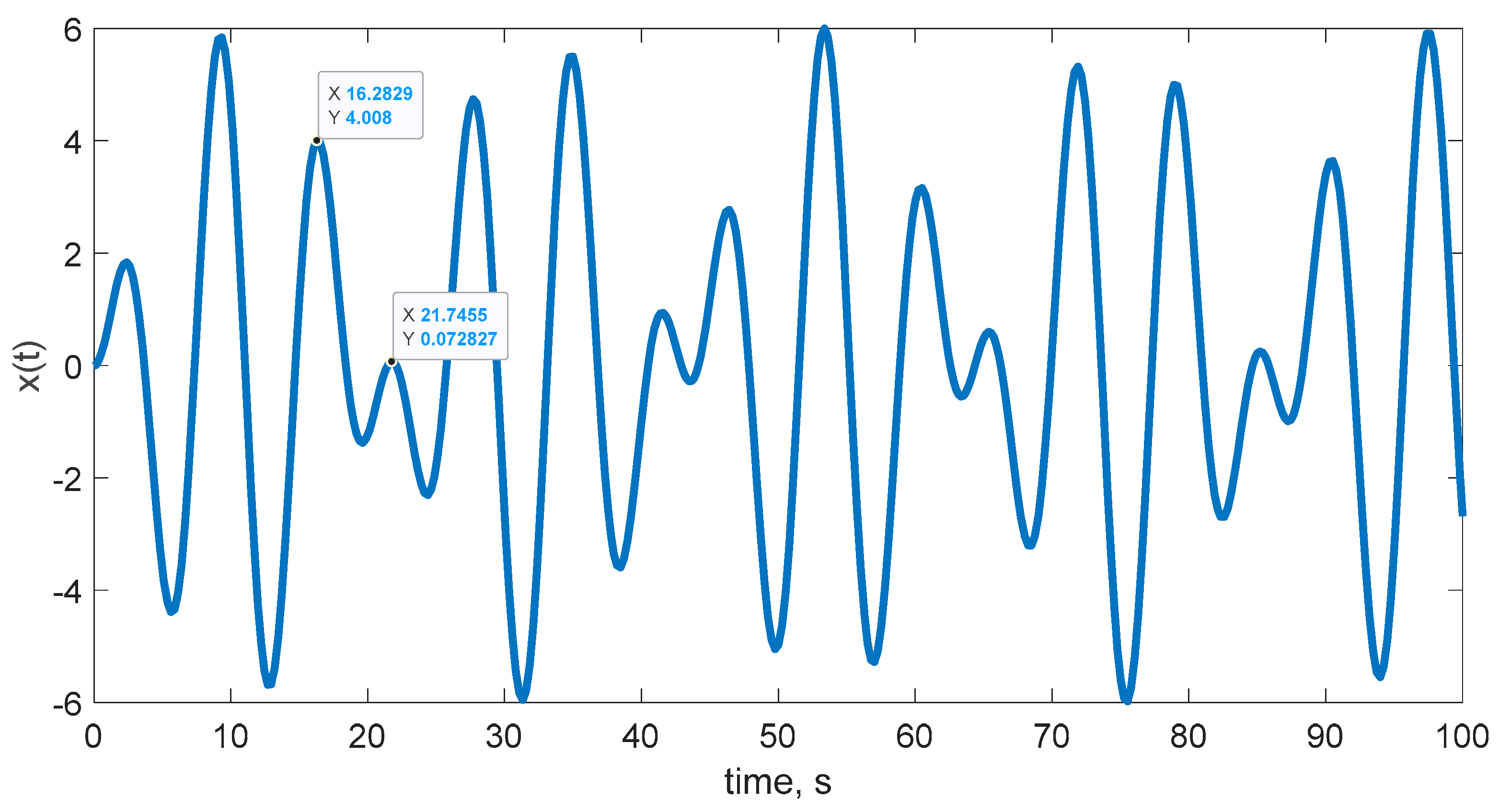
3.1. An Undamped Forced Oscillator
3.2. Non-Linear Soil Consolidation
4. Discussion
5. Conclusions
Author Contributions
Funding
Data Availability Statement
Conflicts of Interest
References
- Del Cerro Velázquez, F.; Gómez-Lopera, S.A.; Alhama, F. A powerful and versatile educational software to simulate transient heat transfer processes in simple fins. Comput. Appl. Eng. Educ. 2008, 16, 72–82. [Google Scholar] [CrossRef]
- Manteca, I.A.; Meca, A.S.; López, F.A. FATSIM-A: An educational tool based on electrical analogy and the code PSPICE to simulate fluid flow and solute transport processes. Comput. Appl. Eng. Educ. 2014, 22, 516–528. [Google Scholar] [CrossRef]
- Campo, A.; Alhama, F. The RC analogy provides a versatile computational tool for unsteady, unidirectional heat conduction in regular solid bodies cooled by adjoining fluids. Int. J. Mech. Eng. Educ. 2003, 31, 233–244. [Google Scholar] [CrossRef]
- Alhama, F.; Campo, A. Utilization of the PSPICE code for the unsteady thermal response of composite walls in a heat transfer course. Int. J. Mech. Eng. Educ. 2003, 31, 359–369. [Google Scholar] [CrossRef]
- Holzbecher, E.O. Modeling Density-Driven Flow in Porous Media; Springer: Berlin/Heidelberg, Germany, 1998. [Google Scholar] [CrossRef]
- Zimparov, V.D.; Petkov, V.M. Application of Discriminated Dimensional Analysis to Low Reynolds Number Swirl Flows in Circular Tubes with Twisted-Tape Inserts. Pressure Drop Correlations. 2009. Available online: https://www.researchgate.net/publication/306094649 (accessed on 20 September 2023).
- Capobianchi, M.; Aziz, A. A scale analysis for natural convective flows over vertical surfaces. Int. J. Therm. Sci. 2012, 54, 82–88. [Google Scholar] [CrossRef]
- Cánovas, M.; Alhama, I.; Alhama, F. Mathematical characterization of bénard-type geothermal scenarios using discriminated non-dimensionalization of the governing equations. Int. J. Nonlinear Sci. Numer. Simul. 2015, 16, 23–34. [Google Scholar] [CrossRef]
- Buckingham, E. On Physically Similar Systems; Illustrations of the Use of Dimensional Equations. Phys. Rev. 1914, 4, 345. [Google Scholar] [CrossRef]
- Henry, L. Langhaar. In Dimensional Analysis and Theory of Models; R E Krieger Publisihng Company: Malabar, FL, USA, 1983. [Google Scholar]
- Fernández-Gracía, M.; Sánchez-Pérez, J.F.; del Cerro, F.; Conesa, M. Mathematical Model to Calculate Heat Transfer in Cylindrical Vessels with Temperature-Dependent Materials. Axioms 2023, 12, 335. [Google Scholar] [CrossRef]
- Alhama, I.; Cánovas, M.; Alhama, F. Simulation of fluid flow and heat transport coupled processes using fahet software. J. Porous Media 2015, 18, 537–546. [Google Scholar] [CrossRef]
- Alhama, I.; Morales, J.L.; Alhama, F. Network models for the numerical solution of coupled ordinary non-lineal differential equations. In Proceedings of the Computational Methods for Coupled Problems in Science and Engineering V—A Conference Celebrating the 60th Birthday of Eugenio Onate, COUPLED PROBLEMS 2013, Ibiza, Spain, 17–19 June 2013; pp. 1407–1417. Available online: https://www.scopus.com/inward/record.uri?eid=2-s2.0-84906846719&partnerID=40&md5=66d157d6572b6c2165bbb40618a43753 (accessed on 20 September 2023).
- Vera, M.P.; Yakhlef, F.; Cintas, M.R.; Lopez, O.C.; Dubujet, P.; Khamlichi, A.; Bezzazi, M. Analytical solution of coupled soil erosion and consolidation equations by asymptotic expansion approach. Appl. Math. Model. 2014, 38, 4086–4098. [Google Scholar] [CrossRef]
- Pérez, J.F.S.; Conesa, M.; Alhama, I.; Alhama, F.; Cánovas, M. Searching fundamental information in ordinary differential equations. Nondimensionalization technique. PLoS ONE 2017, 12, e0185477. [Google Scholar] [CrossRef]
- Alhama, I.; Cánovas, M.; Alhama, F. On the nondimensionalization process in complex problems: Application to natural convection in anisotropic porous media. Math. Probl. Eng. 2014, 2014, 796781. [Google Scholar] [CrossRef]
- Conesa, M.; Pérez, J.F.S.; Alhama, I.; Alhama, F. On the nondimensionalization of coupled, nonlinear ordinary differential equations. Nonlinear Dyn. 2016, 84, 91–105. [Google Scholar] [CrossRef]
- González-Fernández, C.F.; y Alhama, F. Heat Transfer and the Network Simulation Method; Horno, J., Ed.; Transworld Research Network: Trivandrum, India, 2001. [Google Scholar]
- JSánchez-Pérez, F.; Motos-Cascales, G.; Conesa, M.; Moral-Moreno, F.; Castro, E.; García-Ros, G. Design of a Thermal Measurement System with Vandal Protection Used for the Characterization of New Asphalt Pavements through Discriminated Dimensionless Analysis. Mathematics 2022, 10, 1924. [Google Scholar] [CrossRef]
- González-Fernández, C.F. Applications of the Network Simulation Method to Transport Processes; Horno, J., Ed.; Transworld Research Network: Trivandrum, India, 2001. [Google Scholar]
- Marín, F.; Alhama, F.; Moreno, J.A. Modelling of nanoscale friction using network simulation method. Comput. Mater. Contin. 2014, 43, 1–19. [Google Scholar]
- Sánchez-Pérez, J.F.; Conesa, M.; Alhama, I.; Cánovas, M. Study of Lotka-Volterra biological or chemical oscillator problem using the normalization technique: Prediction of time and concentrations. Mathematics 2020, 8, 1324. [Google Scholar] [CrossRef]
- Sánchez-Pérez, J.F.; García-Ros, G.; Conesa, M.; Castro, E.; Cánovas, M. Methodology to Obtain Universal Solutions for Systems of Coupled Ordinary Differential Equations: Examples of a Continuous Flow Chemical Reactor and a Coupled Oscillator. Mathematics 2023, 11, 2303. [Google Scholar] [CrossRef]
- Sánchez-Pérez, J.F.; Alhama, I. Universal curves for the solution of chlorides penetration in reinforced concrete, water-saturated structures with bound chloride. Commun. Nonlinear Sci. Numer. Simul. 2020, 84, 105201. [Google Scholar] [CrossRef]
- Horno, J.; García-Hernández, M.T.; González-Fernández, C.F. Digital simulation of electrochemical processes by the network approach. J. Electroanal. Chem. 1993, 352, 83–97. [Google Scholar] [CrossRef]
- de Mesa, A.G. Oscilaciones y Ondas; Universidad Nacional de Colombia: Bogotá, Colombia, 2005. [Google Scholar]
- Cardozo, J.; Jean, L.; Castro, P.; Muñoz, J.H. Estudio del sistema masa-resorte utilizando Mathematica: Study of the spring-mass system using Mathematica. Noria Investig. Educ. 2021, 2. [Google Scholar]
- De, I.; Piña, J.; Instituto, V.; Nacional, P. Análisis de Movimiento de Sistemas Oscilantes Forzados. 2019. Available online: https://www.researchgate.net/publication/334114737 (accessed on 20 September 2023).
- García-Ros, G. Caracterización Adimensional y Simulación Numérica de Procesos Lineales y No Lineales de Consolidación de Suelos. Doctoral Dissertation, Universidad Politécnica de Cartagena, Cartagena, Spain, 2016. [Google Scholar] [CrossRef]
- Manteca, I.A.; García-Ros, G.; López, F.A. Universal solution for the characteristic time and the degree of settlement in nonlinear soil consolidation scenarios. A deduction based on nondimensionalization. Commun. Nonlinear Sci. Numer. Simul. 2018, 57, 186–201. [Google Scholar] [CrossRef]
- Davis, E.H.; Raymond, G.P. A non-linear theory of consolidation. Geotechnique 1965, 15, 161–173. [Google Scholar] [CrossRef]
- Juárez-Badillo, E.; Chen, B. Consolidation Curves for Clays. J. Geotech. Eng. 1983, 109, 1303–1312. [Google Scholar] [CrossRef]
- Cornetti, P.; Battaglio, M. Nonlinear consolidation of soil modeling and solution techniques. Math. Comput. Model. 1994, 20, 1–12. [Google Scholar] [CrossRef]
- Arnod, S.; Battaglio, M.; Bbllomo, N. Nonlinear models in soils consolidation theory parameter sensitivity analysis. Math. Comput. Model. 1996, 24, 11–20. [Google Scholar] [CrossRef]
- Unesi, M.; Noaparast, M.; Shafaei, S.Z.; Jorjani, E. The role of ore properties in thickening process. Physicochem. Probl. Miner. Process. 2014, 50, 783–794. [Google Scholar] [CrossRef]
- Wu, A.; Ruan, Z.; Bürger, R.; Yin, S.; Wang, J.; Wang, Y. Optimization of flocculation and settling parameters of tailings slurry by response surface methodology. Miner. Eng. 2020, 156, 106488. [Google Scholar] [CrossRef]
- Benn, F.A.; Fawell, P.D.; Halewood, J.; Austin, P.J.; Costine, A.D.; Jones, W.G.; Francis, N.S.; Druett, D.C.; Lester, D. Sedimentation and consolidation of different density aggregates formed by polymer-bridging flocculation. Chem. Eng. Sci. 2018, 184, 111–125. [Google Scholar] [CrossRef]
- Gladman, B.R.; Rudman, M.; Scales, P.J. Experimental validation of a 1-D continuous thickening model using a pilot column. Chem. Eng. Sci. 2010, 65, 3937–3946. [Google Scholar] [CrossRef]


| −1 | −1 | −1 | |
| −1 | −1 | −1 | |
| −0.998 | −1 | −0.998 | |
| 0.836 | 0.871 | 0.836 |
| π2,A | 0.1 | 0.1 | 0.2 | 0.3 | 0.4 | 0.6 | 0.8 | 1.0 | 1.2 | 1.4 | 2.0 | 5.0 | 10.0 | 20.0 | 30.0 |
| π1,A | 15.0 | 13.8 | 8.1 | 6.0 | 4.8 | 3.5 | 2.8 | 2.4 | 2.1 | 1.8 | 1.4 | 0.7 | 0.4 | 0.2 | 0.2 |
| 0.01 | 0.05 | 0.1 | 0.5 | 1 | 2 | 10 | 20 | 40 | 50 | |
| 1.000 | 1.000 | 1.000 | 1.001 | 1.002 | 1.003 | 1.020 | 1.050 | 1.136 | 1.192 |
| Initial Parameters | Simulation Results | Normalization | ||||||||
|---|---|---|---|---|---|---|---|---|---|---|
| Validation | ||||||||||
| 1 | 1 | 1 | 0.1 | 0.6 | 0.29 | 7.37 | 1.8425 | 1 | 0.01044 | 1.8425 |
| 2 | 1 | 1 | 0.1 | 0.9 | 1.04 | 6.58 | 1.6450 | 1 | 0.08424 | 1.6450 |
| 3 | 2 | 2 | 1 | 1.1 | 4.74 | 5.77 | 1.4425 | 1 | 11.4708 | 1.4425 |
| 4 | 2 | 2 | 3 | 1.5 | 2.45 | 3.34 | 0.8350 | 1 | 33.075 | 0.8350 |
| 5 | 2 | 1 | 2 | 0.9 | 6.42 | 7.14 | 1.7850 | 1.414 | 20.8008 | 1.2622 |
| 6 | 2 | 1 | 3 | 0.9 | 5.99 | 5.46 | 1.3650 | 1.414 | 29.1114 | 0.9652 |
| Validation | 1 | 2 | 3 | 5 | 6 | 4 |
|---|---|---|---|---|---|---|
| 3.395 | 2.706 | 2.081 | 1.593 | 0.932 | 0.697 | |
| 0.010 | 0.084 | 11.471 | 20.801 | 29.111 | 33.075 |
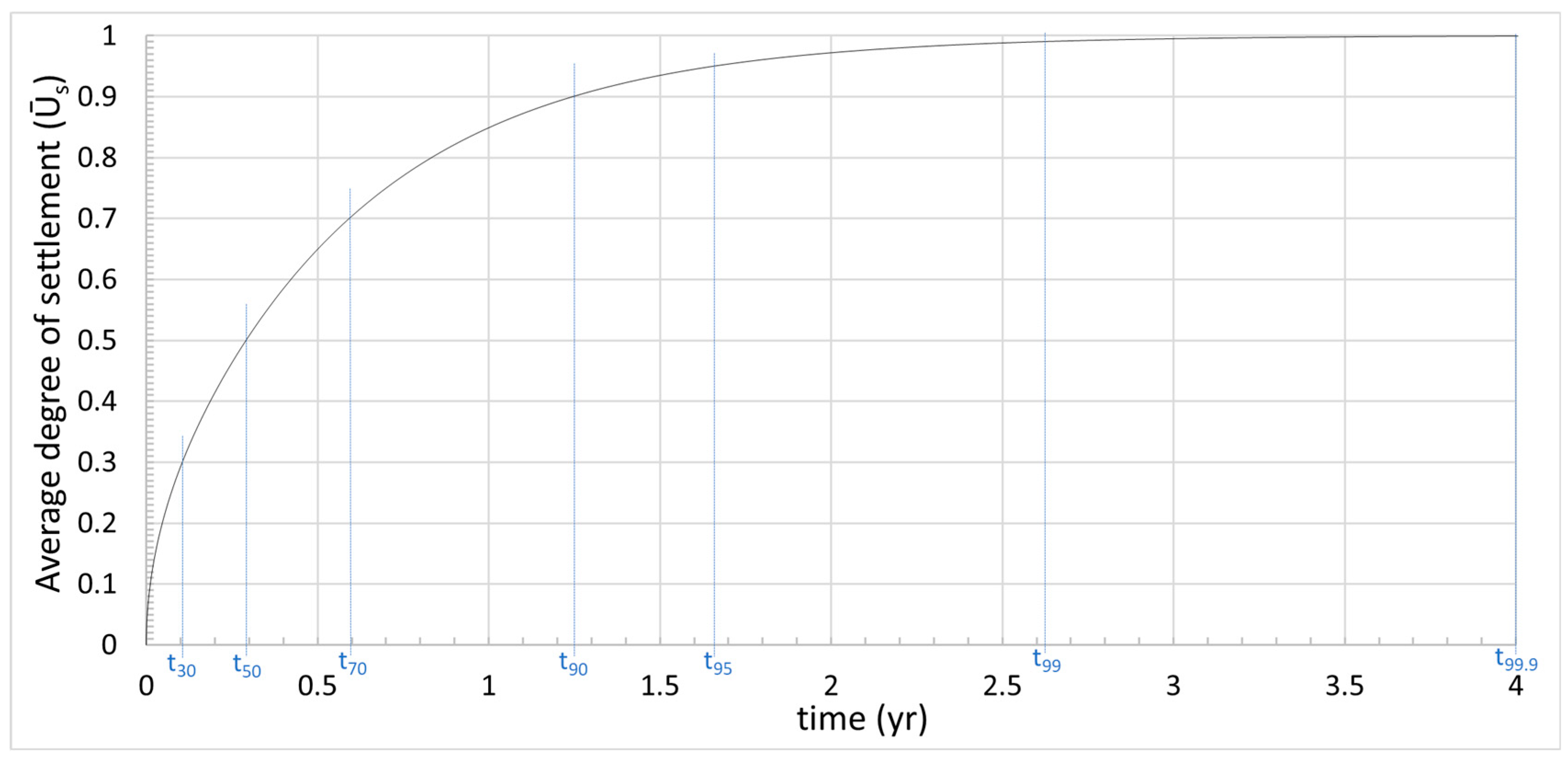
| (%) | 30 | 50 | 70 | 90 | 95 | 99 | 99.9 |
|---|---|---|---|---|---|---|---|
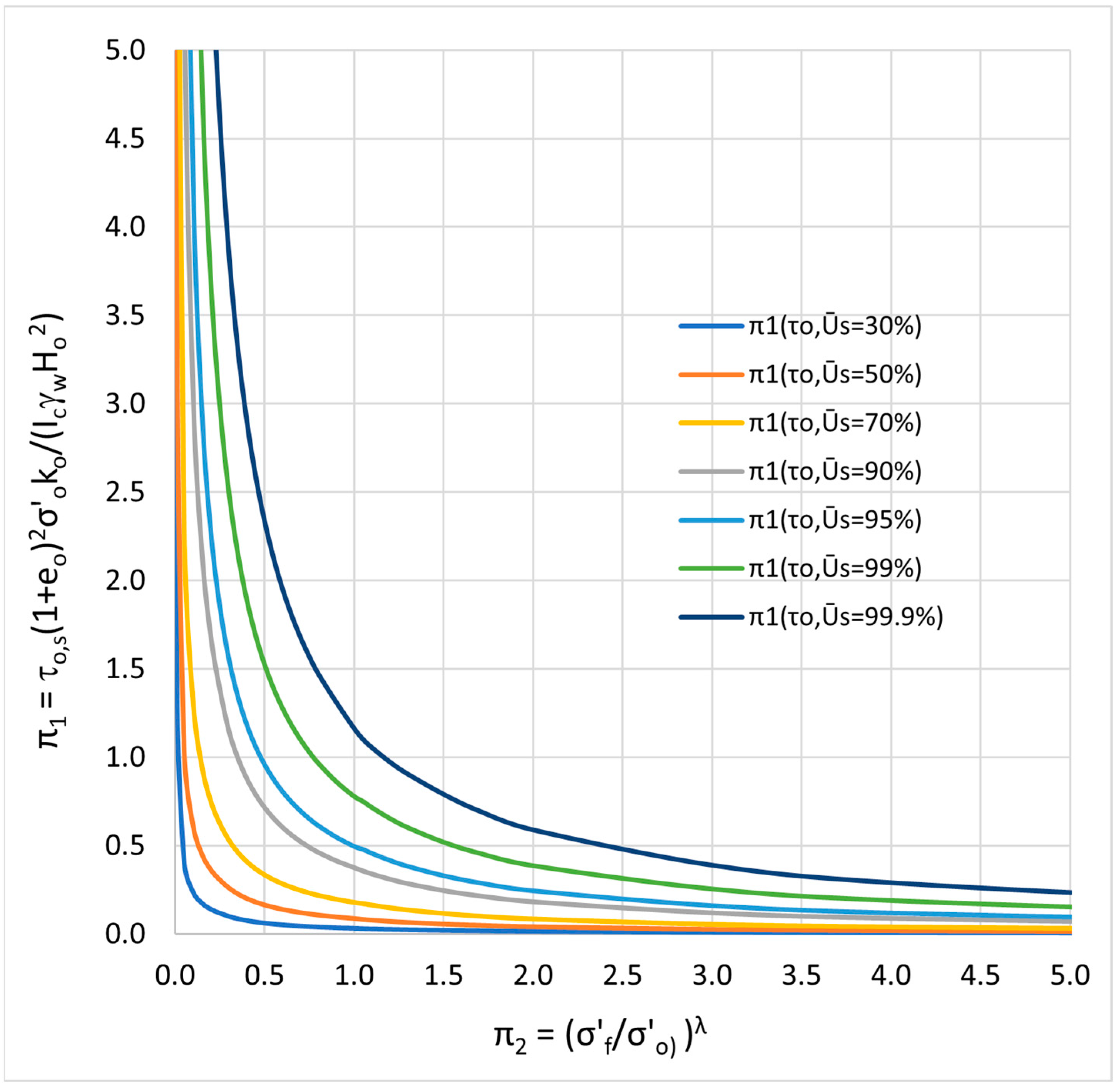
for = 0.8 (Figure 7) | 0.04 | 0.11 | 0.22 | 0.46 | 0.61 | 0.96 | 1.47 |
| (yr) estimated (Figure 7) | 0.1063 | 0.2997 | 0.5995 | 1.2534 | 1.6621 | 2.6158 | 4.0054 |
| (yr) Simulated (Figure 8) | 0.1053 | 0.2976 | 0.5931 | 1.2478 | 1.6620 | 2.6249 | 4.0006 |
| rel. error (%) for | 0.92 | 0.71 | 1.07 | 0.45 | 0.01 | 0.35 | 0.12 |
Disclaimer/Publisher’s Note: The statements, opinions and data contained in all publications are solely those of the individual author(s) and contributor(s) and not of MDPI and/or the editor(s). MDPI and/or the editor(s) disclaim responsibility for any injury to people or property resulting from any ideas, methods, instructions or products referred to in the content. |
© 2023 by the authors. Licensee MDPI, Basel, Switzerland. This article is an open access article distributed under the terms and conditions of the Creative Commons Attribution (CC BY) license (https://creativecommons.org/licenses/by/4.0/).
Share and Cite
Conesa, M.; Sánchez-Pérez, J.F.; García-Ros, G.; Castro, E.; Valenzuela, J. Normalization Method as a Potent Tool for Grasping Linear and Nonlinear Systems in Physics and Soil Mechanics. Mathematics 2023, 11, 4321. https://doi.org/10.3390/math11204321
Conesa M, Sánchez-Pérez JF, García-Ros G, Castro E, Valenzuela J. Normalization Method as a Potent Tool for Grasping Linear and Nonlinear Systems in Physics and Soil Mechanics. Mathematics. 2023; 11(20):4321. https://doi.org/10.3390/math11204321
Chicago/Turabian StyleConesa, Manuel, Juan Francisco Sánchez-Pérez, Gonzalo García-Ros, Enrique Castro, and Julio Valenzuela. 2023. "Normalization Method as a Potent Tool for Grasping Linear and Nonlinear Systems in Physics and Soil Mechanics" Mathematics 11, no. 20: 4321. https://doi.org/10.3390/math11204321
APA StyleConesa, M., Sánchez-Pérez, J. F., García-Ros, G., Castro, E., & Valenzuela, J. (2023). Normalization Method as a Potent Tool for Grasping Linear and Nonlinear Systems in Physics and Soil Mechanics. Mathematics, 11(20), 4321. https://doi.org/10.3390/math11204321