
The New Four-Dimensional Fractional Chaotic Map with Constant and Variable-Order: Chaos, Control and Synchronization
 ,
, 
Abstract
:1. Introduction
2. Fractional Discrete Calculus
Fractional-Order SF-SIMM with Discrete-Time
3. Dynamical Properties of SF-SIMM with Discrete Time
3.1. Complexity of Discrete Fractional-Order SF-SIMM
- The discrete Fourier transform of the sequence is determined:
- The mean square value is calculated as:
- We set
- The inverse Fourier transform of is given as follows:Finally, we evaluate the formula of the complexity by:
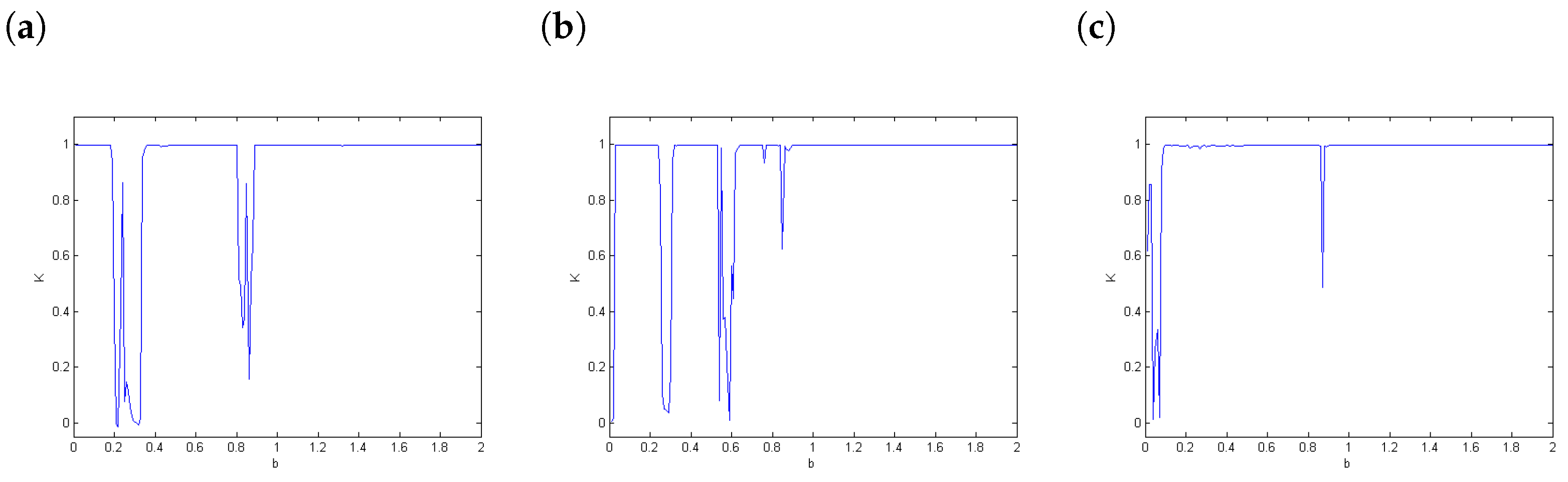
3.2. The 0–1 Test for Chaos
3.3. Control Fractional-Order SF-SIMM Map
3.3.1. Stabilization
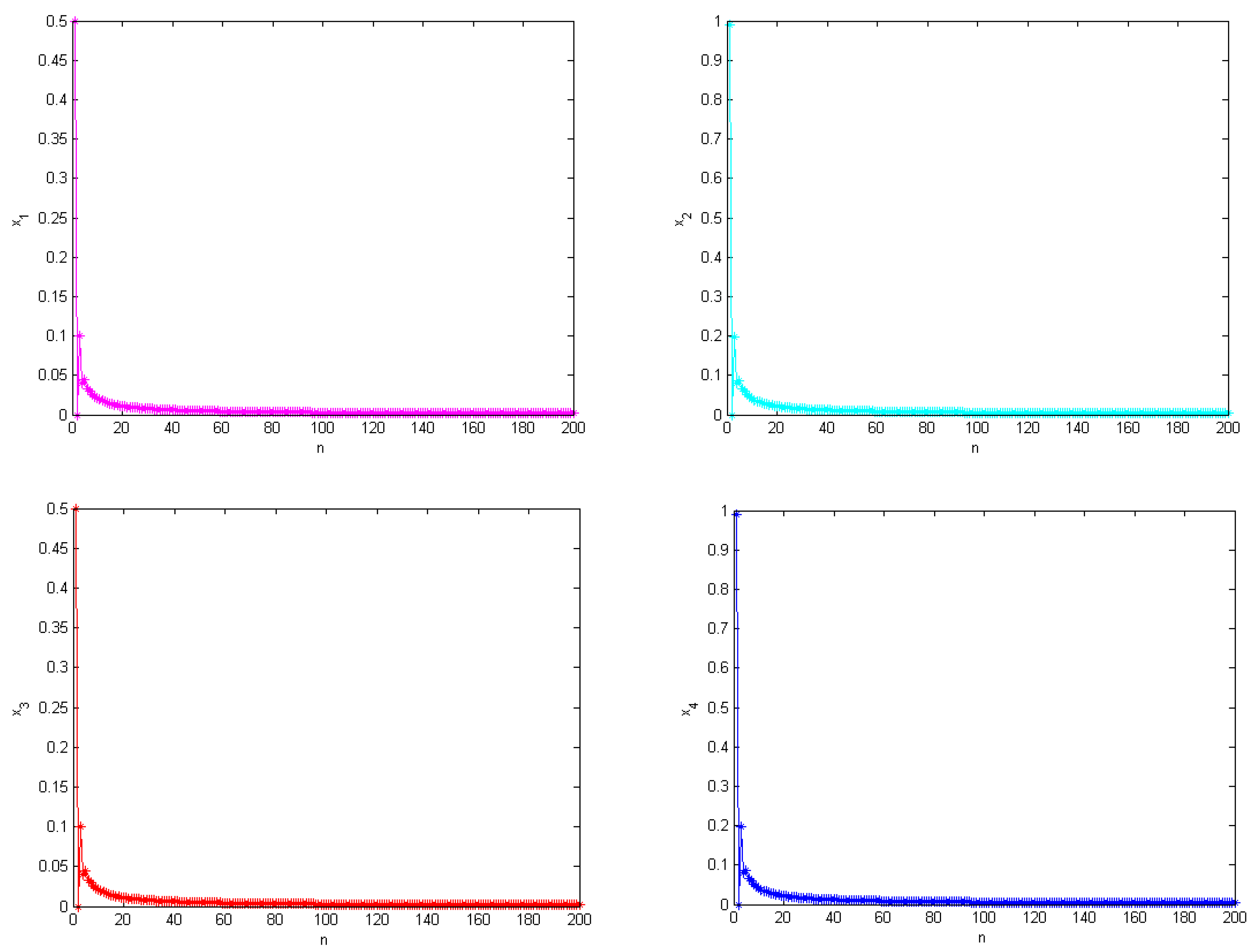
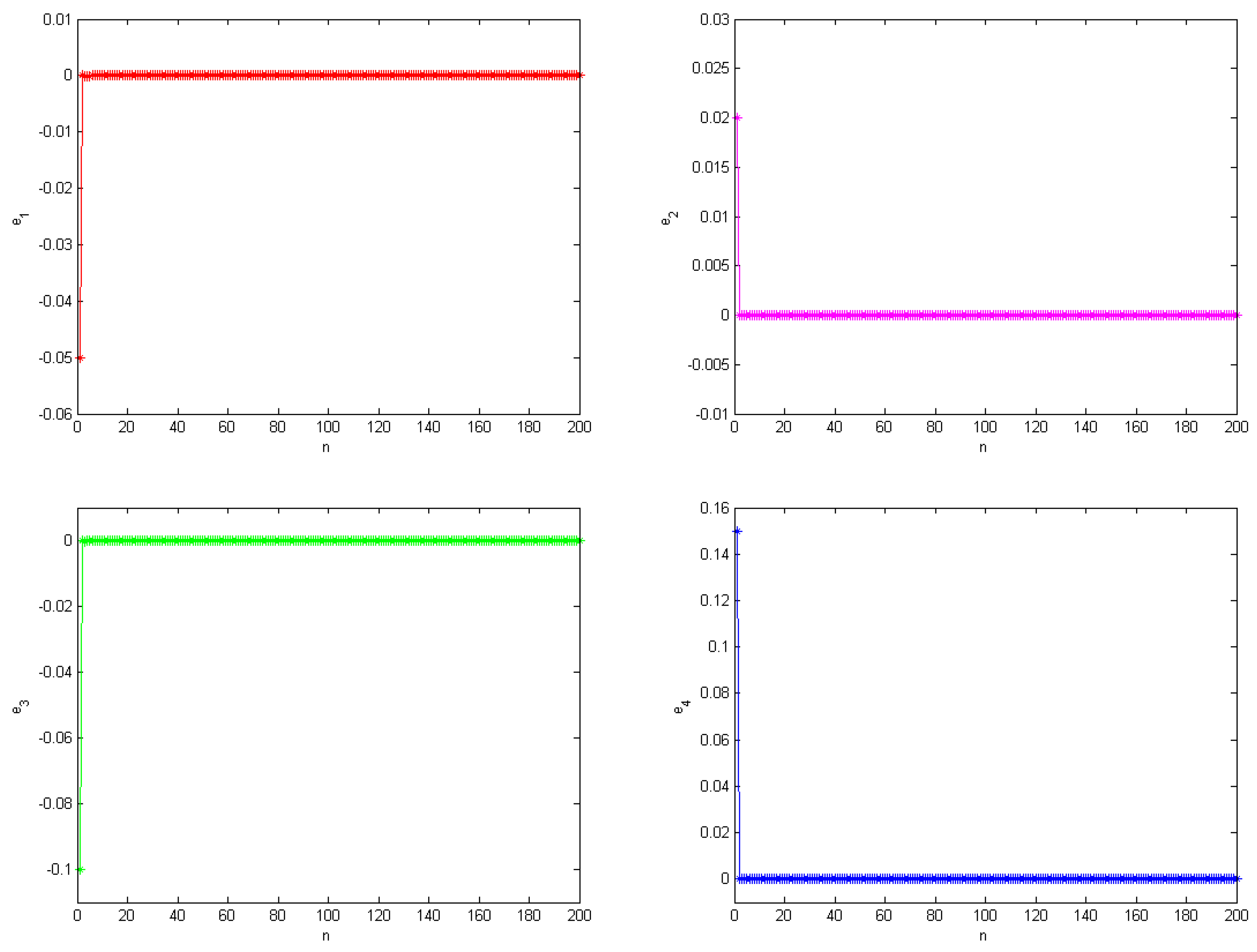
3.3.2. Synchronization
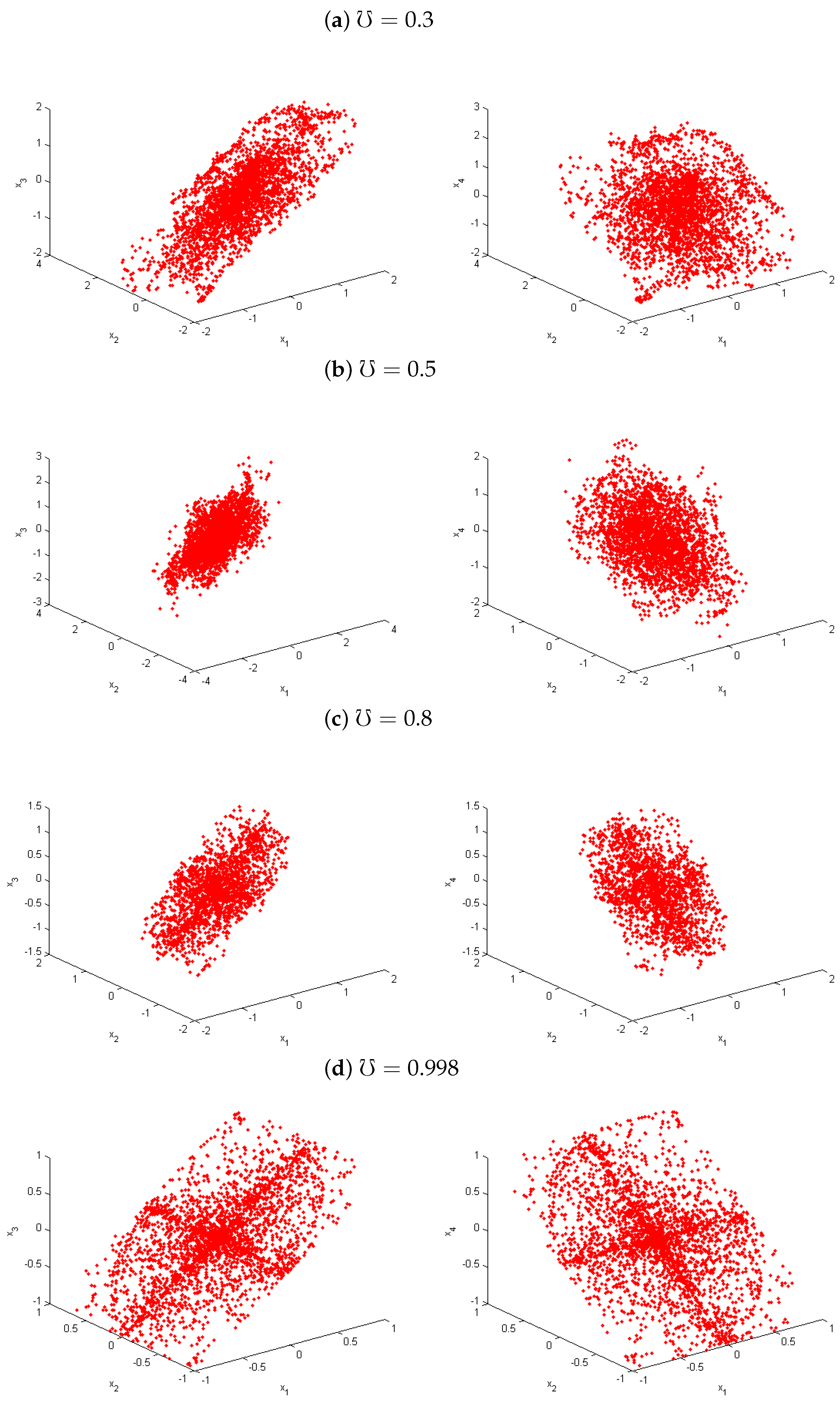
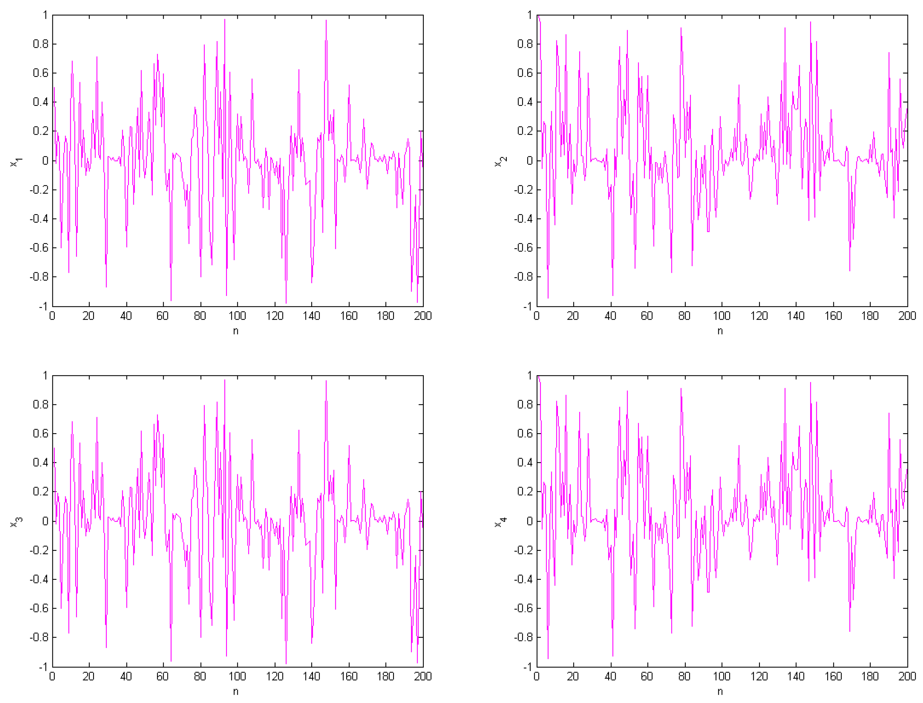
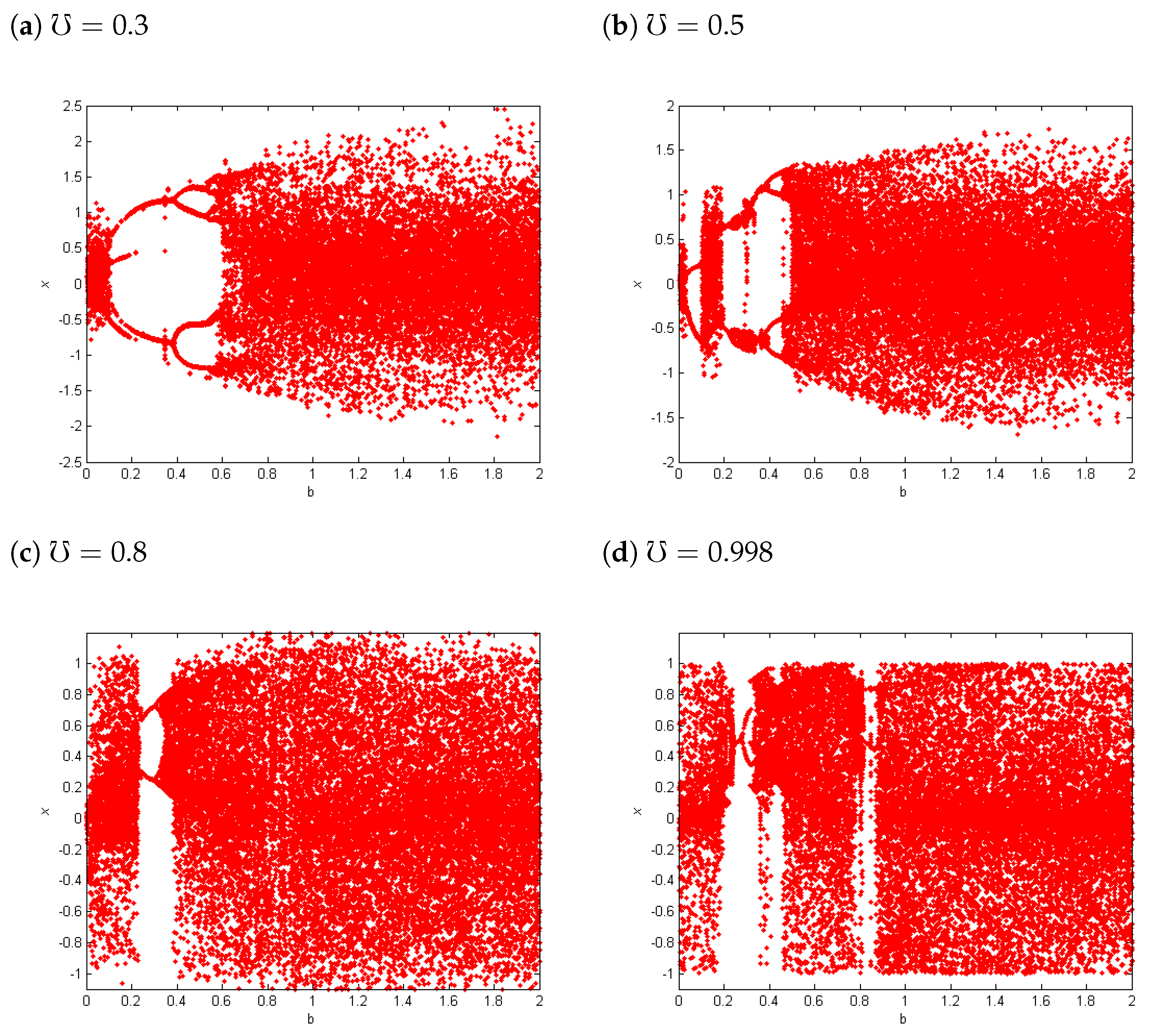
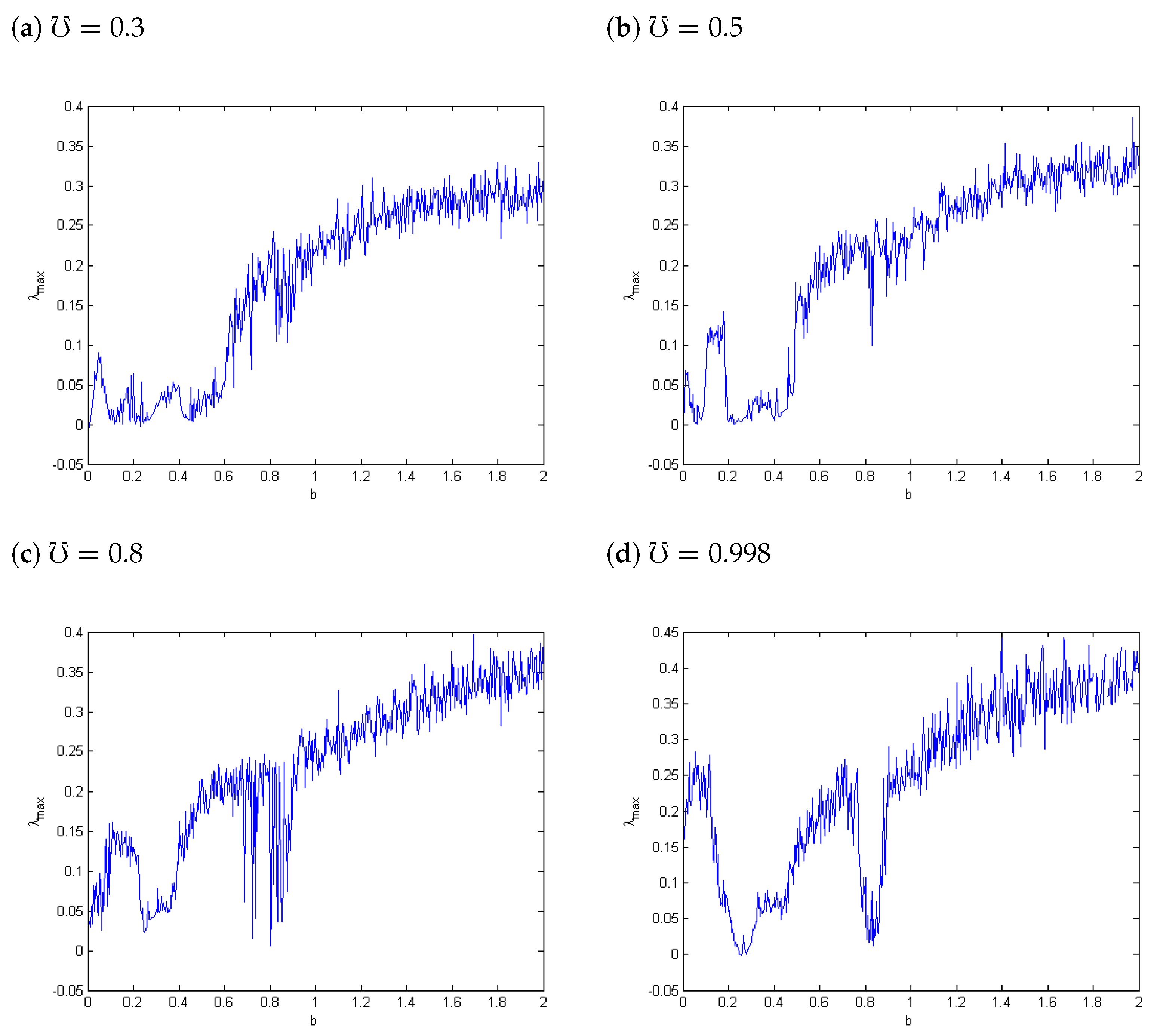
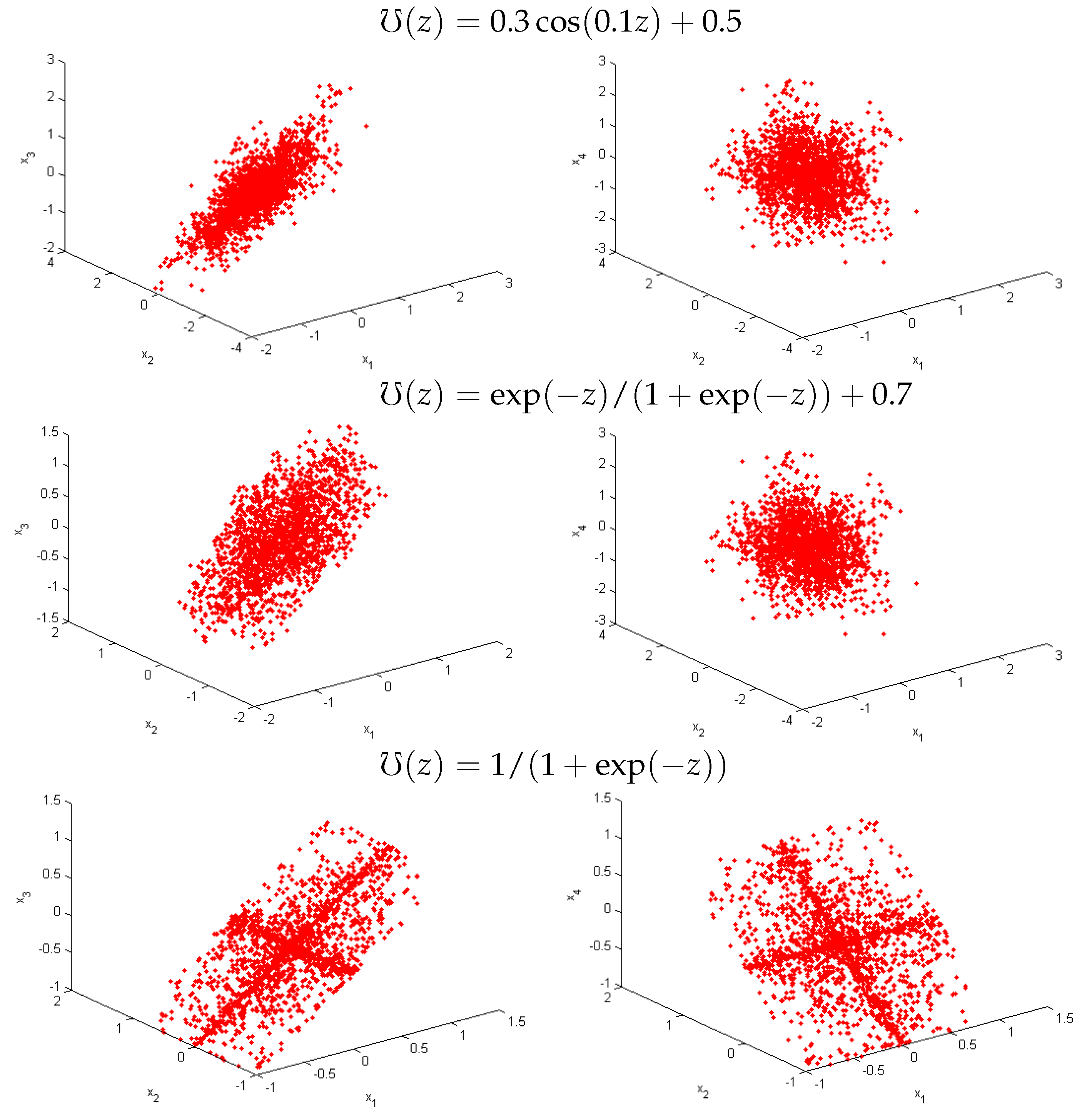
4. Chaos of Variable Fractional SF-SIMM with Discrete-Time
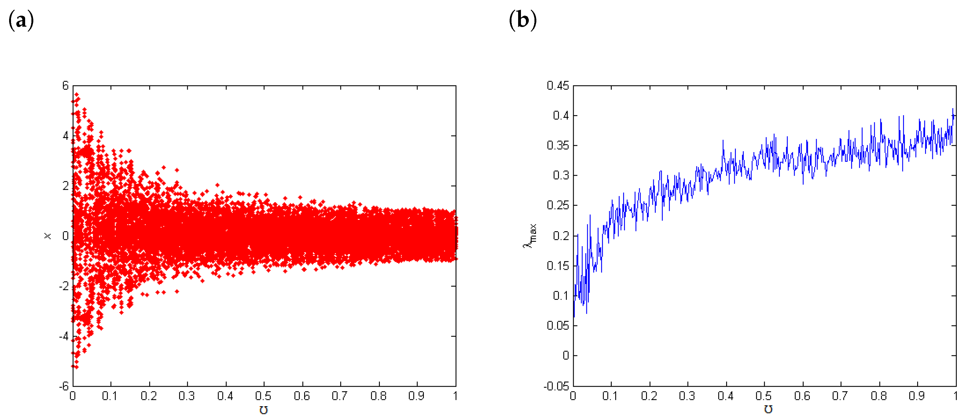
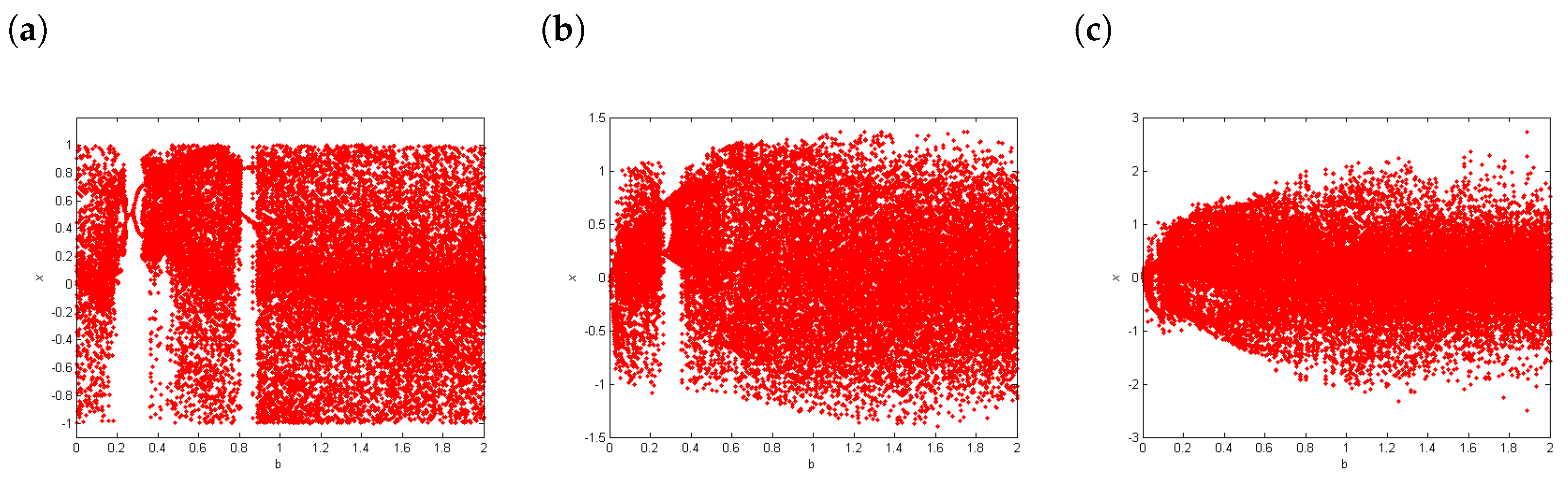
4.1. Largest Lyapunov Exponents () and Bifurcation
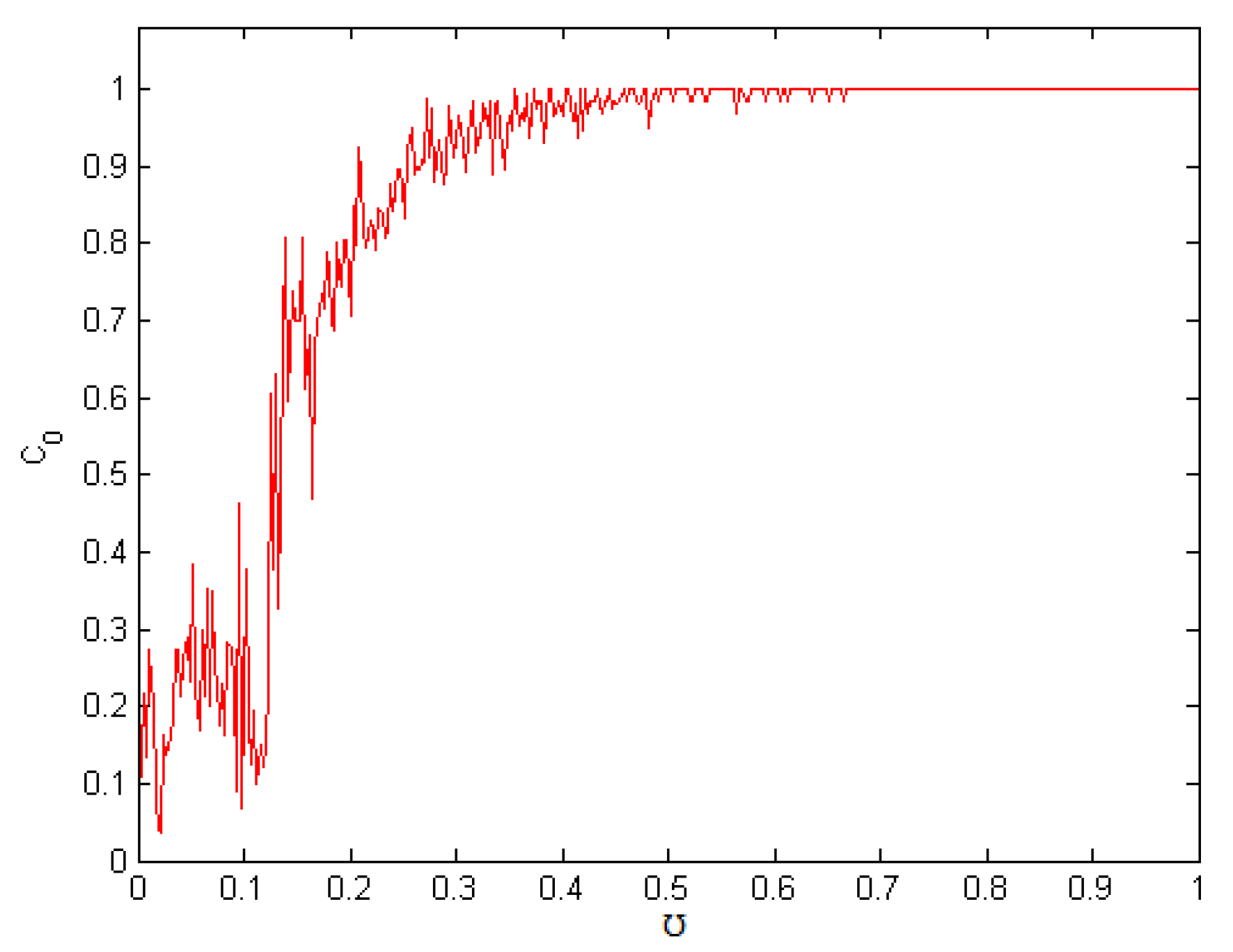
4.2. Complexity
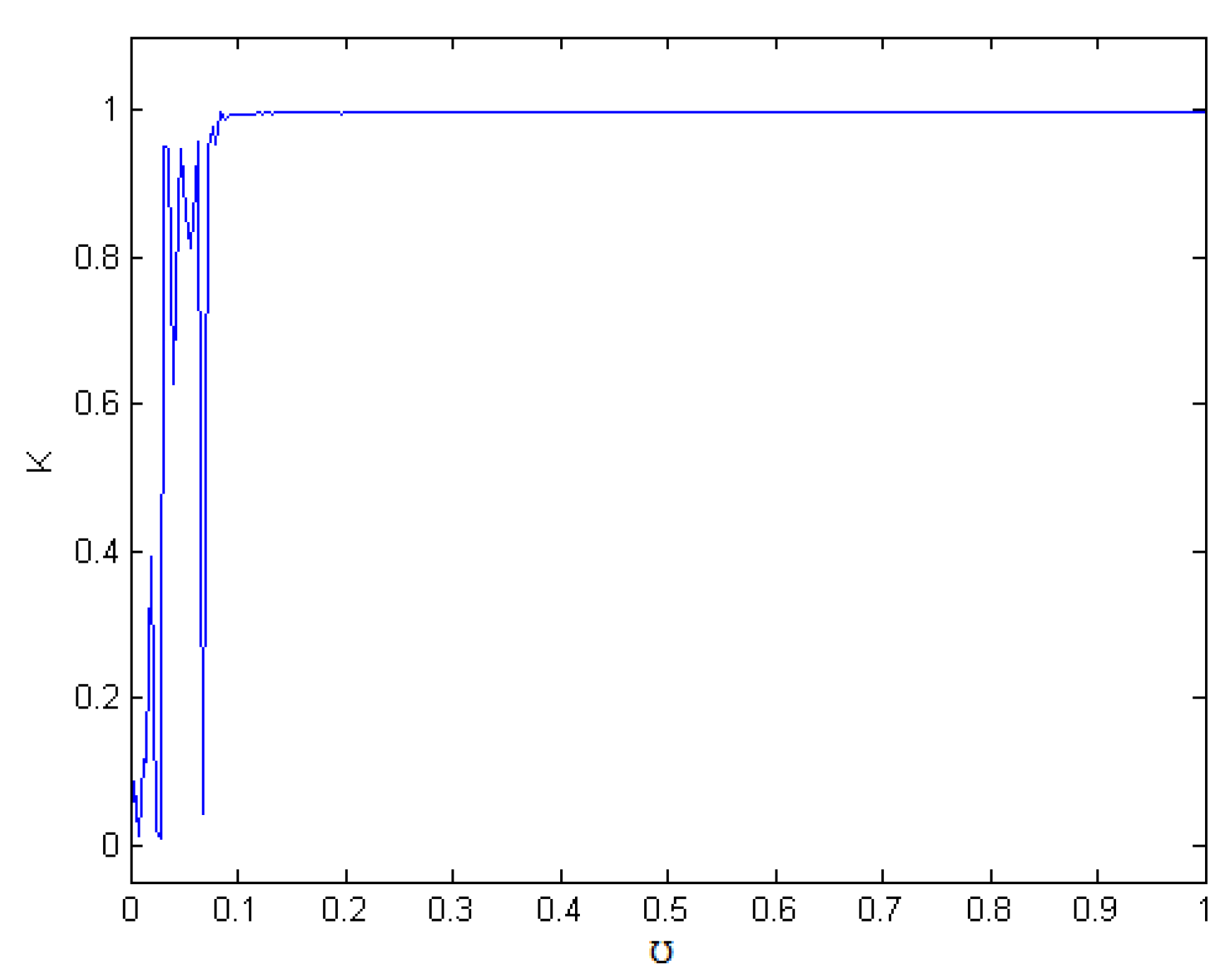
4.3. The 0–1 Test
5. Conclusions and Future Works
Author Contributions
Funding
Institutional Review Board Statement
Informed Consent Statement
Data Availability Statement
Conflicts of Interest
References
- Devaney, R.L.; Alligood, K.T. Chaos and Fractals: The Mathematics behind the Computer Graphics: The Mathematics behind the Computer Graphics; American Mathematical Soc: Providence, RI, USA, 1989; Volume 1, ISBN 9780821801376. [Google Scholar]
- Biswas, H.R.; Hasan, M.M.; Bala, S.K. Chaos theory and its applications in our real life. Barishal Univ. J. Part 2018, 1, 123–140. [Google Scholar]
- Majhi, S.; Perc, M.; Ghosh, D. Dynamics on higher-order networks: A review. J. R. Soc. Interface 2022, 19, 20220043. [Google Scholar] [CrossRef] [PubMed]
- Wu, G.C.; Baleanu, D. Discrete fractional logistic map and its chaos. Nonlinear Dyn. 2014, 75, 283–287. [Google Scholar] [CrossRef]
- Saadeh, R.; Abbes, A.; Al-Husban, A.; Ouannas, A.; Grassi, G. The Fractional Discrete Predator–Prey Model: Chaos, Control and Synchronization. Fractal Fract. 2023, 7, 120. [Google Scholar] [CrossRef]
- Dababneh, A.; Djenina, N.; Ouannas, A.; Grassi, G.; Batiha, I.M.; Jebril, I.H. A new incommensurate fractional-order discrete COVID-19 model with vaccinated individuals compartment. Fractal Fract. 2022, 6, 456. [Google Scholar] [CrossRef]
- Chen, M.; Sun, M.; Bao, H.; Hu, Y.; Bao, B. Flux–charge analysis of two-memristor-based Chua’s circuit: Dimensionality decreasing model for detecting extreme multistability. IEEE Trans. Ind. Electron. 2019, 67, 2197–2206. [Google Scholar] [CrossRef]
- Almatroud, O.A.; Pham, V.T. Building Fixed Point-Free Maps with Memristor. Mathematics 2023, 11, 1319. [Google Scholar] [CrossRef]
- Chen, L.; Yin, H.; Huang, T.; Yuan, L.; Zheng, S.; Yin, L. Chaos in fractional-order discrete neural networks with application to image encryption. Neural Netw. 2020, 125, 174–184. [Google Scholar] [CrossRef]
- Liu, X.; Mou, J.; Zhang, Y.; Cao, Y. A New Hyperchaotic Map Based on Discrete Memristor and Meminductor: Dynamics Analysis, Encryption Application, and DSP Implementation. IEEE Trans. Ind. Electron. 2023; Early Access. [Google Scholar]
- Bao, H.; Ding, R.; Hua, M.; Wu, H.; Chen, B. Initial-condition effects on a two-memristor-based Jerk system. Mathematics 2022, 10, 411. [Google Scholar] [CrossRef]
- Wang, J.; Gu, Y.; Rong, K.; Xu, Q.; Zhang, X. Memristor-based Lozi map with hidden hyperchaos. Mathematics 2022, 10, 3426. [Google Scholar] [CrossRef]
- Ouannas, A.; Khennaoui, A.A.; Grassi, G.; Bendoukha, S. On chaos in the fractional–order Grassi–Miller map and its control. J. Comput. Appl. Math. 2019, 358, 293–305. [Google Scholar] [CrossRef]
- Wang, L.; Sun, K.; Peng, Y.; He, S. Chaos and complexity in a fractional-order higher-dimensional multicavity chaotic map. Chaos Solitons Fractals 2020, 131, 109488. [Google Scholar] [CrossRef]
- Peng, Y.; He, S.; Sun, K. Chaos in the discrete memristor-based system with fractional-order difference. Results Phys. 2021, 24, 104106. [Google Scholar] [CrossRef]
- Lu, Y.M.; Wang, C.H.; Deng, Q.L.; Xu, C. The dynamics of a memristor-based Rulkov neuron with the fractional-order difference. Chin. Phys. B 2022. [Google Scholar] [CrossRef]
- Batiha, I.M.; Albadarneh, R.B.; Momani, S.; Jebril, I.H. Dynamics analysis of fractional-order Hopfeld neural networks. Int. J. Biomath. 2020, 13, 2050083. [Google Scholar] [CrossRef]
- Ma, M.; Lu, Y.; Li, Z.; Sun, Y.; Wang, C. Multistability and Phase Synchronization of Rulkov Neurons Coupled with a Locally Active Discrete Memristor. Fractal Fract. 2023, 7, 82. [Google Scholar] [CrossRef]
- Peng, Y.; Liu, J.; He, S.; Sun, K. Discrete fracmemristor-based chaotic map by Grunwald–Letnikov difference and its circuit implementation. Chaos Solitons Fractals 2023, 171, 113429. [Google Scholar] [CrossRef]
- Vignesh, D.; Banerjee, S. Dynamical analysis of a fractional discrete-time vocal system. Nonlinear Dyn. 2022, 111, 4501–4515. [Google Scholar] [CrossRef]
- Abbes, A.; Ouannas, A.; Shawagfeh, N.; Khennaoui, A.A. Incommensurate fractional discrete neural network: Chaos and complexity. Eur. Phys. J. Plus 2022, 137, 235. [Google Scholar] [CrossRef]
- Al-Saidi, N.M.; Natiq, H.; Baleanu, D.; Ibrahim, R.W. The dynamic and discrete systems of variable fractional order in the sense of the Lozi structure map. AIMS Math. 2023, 8, 733–751. [Google Scholar] [CrossRef]
- Karoun, R.C.; Ouannas, A.; Al Horani, M.; Grassi, G. The Effect of Caputo Fractional Variable Difference Operator on a Discrete-Time Hopfield Neural Network with Non-Commensurate Order. Fractal Fract. 2022, 6, 575. [Google Scholar] [CrossRef]
- Ahmed, S.B.; Ouannas, A.; Horani, M.A.; Grassi, G. The Discrete Fractional Variable-Order Tinkerbell Map: Chaos, 0–1 Test, and Entropy. Mathematics 2022, 10, 3173. [Google Scholar] [CrossRef]
- Huang, L.L.; Park, J.H.; Wu, G.C.; Mo, Z.W. Variable-order fractional discrete-time recurrent neural networks. J. Comput. Appl. Math. 2020, 370, 112633. [Google Scholar] [CrossRef]
- Peng, Y.; Sun, K.; Peng, D.; Ai, W. Dynamics of a higher dimensional fractional-order chaotic map. Phys. A Stat. Mech. Appl. 2022, 525, 96–107. [Google Scholar] [CrossRef]
- Abdeljawad, T. On Riemann and Caputo fractional differences. Comput. Math. Appl. 2011, 62, 1602–1611. [Google Scholar] [CrossRef]
- Atici, F.; Eloe, P.W. Discrete fractional calculus with the nabla operator. Electron. J. Qual. Theory Differ. Equ. 2009, 3, 1–12. [Google Scholar] [CrossRef]
- Anastassiou, G.A. Principles of delta fractional calculus on time scales and inequalities. Math. Comput. Model. 2022, 52, 556–566. [Google Scholar] [CrossRef]
- Čermák, J.; Győri, I.; Nechvátal, L. On explicit stability conditions for a linear fractional difference system. Fract. Calc. Appl. Anal. 2015, 18, 651–672. [Google Scholar] [CrossRef]
- Wu, G.C.; Baleanu, D. Jacobian matrix algorithm for Lyapunov exponents of the discrete fractional maps. Commun. Nonlinear Sci. Numer. Simulat. 2015, 22, 95–100. [Google Scholar] [CrossRef]
- Ran, J. Discrete chaos in a novel two-dimensional fractional chaotic map. Adv. Differ. Equ. 2018, 2018, 294. [Google Scholar] [CrossRef]
- Gottwald, G.A.; Melbourne, I. A new test for chaos in deterministic systems. Proc. Math. Phys. Eng. Sci. 2004, 460, 603–611. [Google Scholar] [CrossRef]


Disclaimer/Publisher’s Note: The statements, opinions and data contained in all publications are solely those of the individual author(s) and contributor(s) and not of MDPI and/or the editor(s). MDPI and/or the editor(s) disclaim responsibility for any injury to people or property resulting from any ideas, methods, instructions or products referred to in the content. |
© 2023 by the authors. Licensee MDPI, Basel, Switzerland. This article is an open access article distributed under the terms and conditions of the Creative Commons Attribution (CC BY) license (https://creativecommons.org/licenses/by/4.0/).
Share and Cite
Hamadneh, T.; Ahmed, S.B.; Al-Tarawneh, H.; Alsayyed, O.; Gharib, G.M.; Al Soudi, M.S.; Abbes, A.; Ouannas, A. The New Four-Dimensional Fractional Chaotic Map with Constant and Variable-Order: Chaos, Control and Synchronization. Mathematics 2023, 11, 4332. https://doi.org/10.3390/math11204332
Hamadneh T, Ahmed SB, Al-Tarawneh H, Alsayyed O, Gharib GM, Al Soudi MS, Abbes A, Ouannas A. The New Four-Dimensional Fractional Chaotic Map with Constant and Variable-Order: Chaos, Control and Synchronization. Mathematics. 2023; 11(20):4332. https://doi.org/10.3390/math11204332
Chicago/Turabian StyleHamadneh, Tareq, Souad Bensid Ahmed, Hassan Al-Tarawneh, Omar Alsayyed, Gharib Mousa Gharib, Maha S. Al Soudi, Abderrahmane Abbes, and Adel Ouannas. 2023. "The New Four-Dimensional Fractional Chaotic Map with Constant and Variable-Order: Chaos, Control and Synchronization" Mathematics 11, no. 20: 4332. https://doi.org/10.3390/math11204332