Abstract
Segmentation of pneumonia on lung radiographs is vital for the precise diagnosis and monitoring of the disease. It enables healthcare professionals to locate and quantify the extent of infection, guide treatment decisions, and improve patient care. One of the most-employed approaches to effectively segment pneumonia in lung radiographs is to treat it as an optimization task. By formulating the problem in this manner, it is possible to use the interesting capabilities of metaheuristic methods to determine the optimal segmentation solution. Although these methods produce interesting results, they frequently produce suboptimal solutions owing to the lack of exploration of the search space. In this paper, a new segmentation method for segmenting pneumonia in lung radiographs is introduced. The algorithm is based on the jellyfish search optimizer (JSO), which is characterized by its excellent global exploration capability and robustness. This method uses an energy curve based on cross-entropy as a cost function that penalizes misclassified pixels more heavily, leading to a sharper focus on regions where segmentation errors occur. This is particularly important because it allows for the accurate delineation of objects or regions of interest. To validate our proposed approach, we conducted extensive testing on the most widely available datasets. The results of our method were compared with those obtained using other established techniques. The results of our evaluation demonstrate that our approach consistently outperforms the other methods at levels 8, 16, and 32, with a difference of more than 10%.
Keywords:
image segmentation; medical image; jellyfish search optimizer; metaheuristic methods; pneumonia MSC:
37N40
1. Introduction
Pneumonia has a significant impact on public health worldwide, particularly in vulnerable populations such as children, the elderly, and individuals with compromised immune systems [1]. It is a leading cause of morbidity and mortality, placing a substantial burden on healthcare systems and economies.
The classical methods for diagnosing pneumonia [2] typically involve a combination of clinical assessment, patient history, physical examination, and traditional imaging techniques, such as radiography or chest radiography.
Assessing pneumonia visually through X-rays or chest radiographs poses challenges owing to the subtle and variable radiographic features of the disease [3]. Pneumonia can mimic other lung conditions, making it difficult to distinguish it visually. Coexisting medical conditions, overlapping symptoms, and the potential for radiologist variability further complicate accurate diagnosis.
The advantages of using segmentation techniques to detect pneumonia in medical images are significant [3]. These techniques enable the precise identification and isolation of infected regions within the lungs, allowing for an accurate assessment of the extent and severity of the disease. By providing quantitative data, segmentation aids in clinical decision-making, treatment planning, and monitoring of patient progress. This enhances the ability to differentiate pneumonia-related abnormalities from healthy tissues, thereby reducing the risk of misdiagnoses. Automation through segmentation methods improves efficiency and consistency in analysis, offering healthcare professionals valuable support for the early and accurate detection of pneumonia, ultimately leading to improved patient care and outcomes [4].
Segmenting images of pneumonia in X-rays or chest radiographs typically involves image processing and computer vision techniques. Common methods include thresholding to separate infected regions from healthy tissues based on pixel intensity, edge detection to outline the boundaries of lesions, and region growth to cluster pixels with similar characteristics. Recently, approaches have incorporated machine learning, such as convolutional neural networks (CNNs), to automate the segmentation processes [5]. These CNNs are trained on labeled datasets to learn patterns and features indicative of pneumonia [6], thereby allowing for accurate and efficient segmentation [7]. By combining these methods with preprocessing steps to enhance image quality, researchers and healthcare professionals can achieve the reliable and precise segmentation of pneumonia-related abnormalities in radiographic images [8]. UNet [9] is a popular convolutional neural network (CNN) architecture primarily used for image segmentation tasks, particularly in the field of medical image analysis. The original UNet architecture consists of two main parts: an encoder and decoder with a contracting path and an expansive path. Variants of UNet have been developed to improve the original architecture and adapt it to various segmentation tasks. Notable variants include UNet++ [10], ResUNet [11], and DenseUNet [12]. Recently, several methods based on CNNs and deep-learning techniques have been proposed for the detection of pulmonary diseases. Representative examples include those in [13,14]. Although methods based on convolutional neural networks (CNNs) or deep learning have shown promise for segmenting pneumonia in X-rays or chest radiographs, they have some notable disadvantages. CNNs often require substantial amounts of labeled training data, which can be scarce and expensive to obtain, particularly for rare pneumonia cases [15]. Additionally, CNNs may struggle with generalization when applied to diverse patient populations or different imaging settings, potentially leading to inconsistent segmentation results.
An alternative approach to the segmentation of pneumonia images in X-rays or chest radiographs is to consider the segmentation problem as an optimization task and employ metaheuristic methods. These methods iteratively analyze the solution space to determine the optimal segmentation configuration based on an objective function. This approach can effectively tackle the complex nature of the problem, aiding in the precise localization and quantification of pneumonia lesions within radiographic images, ultimately enhancing diagnostic accuracy and clinical decision making. Examples of these approaches include techniques such as particle swarm optimization (PSO) [16], evolutionary arithmetic optimization [17], sunflower optimization [18], and differential evolution [19].
It is important to acknowledge that no single metaheuristic algorithm can solve all optimization problems competitively. The specific strategies employed to solve an optimization problem are influenced by the distinct complexities embedded within its objective function. Some problems require an extensive exploration of the search space, whereas others require a finer focus on the refinement of already explored areas through exploitation mechanisms. Employing a metaheuristic method ill-suited to a specific problem often results in suboptimal solutions. Consequently, identifying the most suitable method requires a comprehensive and systematic evaluation process, wherein several methods are rigorously tested. This evaluation should involve rigorous testing and a statistical assessment of the solutions provided by each method, ultimately leading to the selection of the most appropriate metaheuristic algorithm tailored to the unique characteristics of the optimization problem.
The jellyfish search optimizer (JSO) [20] is a newly developed metaheuristic algorithm that solves complex real-world optimization problems. This is based on the foraging behavior of jellyfish in the ocean. Compared with other metaheuristic methods, the global exploration capability of the JSO algorithm is one of its most important abilities as an optimization technique. Owing to this remarkable characteristic, its use has been extended to different areas such as power systems [21], structural optimization [22], and renewable energy sources [23].
When a problem is formulated as an optimization task to obtain its solution, the fundamental problem is to formulate a suitable objective function. This function must clearly reflect the important details of the solution, as the search algorithm evaluates each candidate solution in terms of this function, providing a value that defines the quality of the solution. Most objective functions used by metaheuristic methods for segmentation include the use of cross-entropy provided by a histogram of intensity levels. Cross-entropy is a versatile mathematical function employed across fields such as information theory, statistics, and machine learning [24]. It serves as a metric for quantifying disparities between the probability distributions (histograms) and models. However, the results obtained with objective functions based on histograms and cross-entropy do not clearly highlight the image details that can be used to contrast and evaluate regions in the images.
In this paper, a novel approach for segmenting pneumonia in lung radiographs is introduced. This method uses the jellyfish search optimizer (JSO) as the optimization method. Unlike other metaheuristic methods, the JSO is known for its strong global exploration capabilities and robustness. With the use of the JSO, there is a better expectation of finding optimal solutions than with the other metaheuristic methods. As an objective function, this approach proposes the use of an energy curve based on cross-entropy as a cost function. This energy curve associates the cross-entropy with the spatial information of the pixels. Therefore, this objective function places greater emphasis on penalizing misclassified pixels, thereby enhancing the precision of delineating regions prone to segmentation errors. This emphasis on accuracy is crucial for identifying objects or regions of interest. To validate the proposed method, extensive testing was conducted using the widely available datasets for pneumonia segmentation. A comparative analysis with established techniques revealed that our approach consistently delivered superior results in terms of both accuracy and robustness, underscoring its potential significance in medical image analysis.
The remainder of this article is organized as follows. Section 2 describes the jellyfish search optimizer (JSO). Section 3 discusses the segmentation procedure under the cross-entropy perspective. Section 4 develops the proposed energy curve as an objective function. Section 5 explains the proposed method. Section 6 presents the experimental results. Finally, Section 7 discusses the conclusions.
2. Jellyfish Search Optimizer (JSO)
The JSO is a novel metaheuristic algorithm inspired by the behavior of jellyfish in the ocean. It was developed by Jui-Sheng Chou and Dinh-Nhat Truong [18,20]. The algorithm simulates the search behavior of jellyfish, which involves their following the ocean current, their motions inside a jellyfish swarm (active and passive motions), a time control mechanism for switching among these movements, and their convergence into jellyfish blooms. The new algorithm has only two control parameters: the population size and the number of iterations. Therefore, the JSO is very simple to use and is potentially an excellent metaheuristic algorithm for solving optimization problems.
The jellyfish population of elements can be characterized and modeled using the following model:
where , and is factor with values within [0,1]. The evaluation of the time control function, , value is conducted following the procedure outlined in Equation (2), and it undergoes a temporal variation, ranging from 0 to 1:
where represents the maximal number of iterations and represents a random uniformly generated number.
When exceeds a fixed value (normally 0.5), the equation provided in Equation (3) is used to calculate the new position for each jellyfish:
where represents the current the best location of the complete population. corresponds to the average position of the population, whereas is a random uniformly distributed number.
When is lower than the threshold, the update of each jellyfish’s position is contingent upon its movement within the swarm, as elucidated in Equations (4) and (5).
where and are the upper bound and lower bounds of the decision variables, respectively. symbolizes a randomly selected element of the population, so that .
If an element moves beyond the boundaries of the search zone, it promptly retraces its path, as exemplified by Equation (6), back to the opposite boundary.
In contrast to conventional classical metaheuristic techniques, the JSO stands out because of its distinctive attributes, particularly its exceptional global exploration capability and robustness. Unlike other methods that may struggle to explore diverse regions of the solution space effectively, the JSO excels in its ability to comprehensively search for optimal solutions across a wide range of possibilities. Its robustness ensures that it can adapt and perform consistently in various problem domains and under different conditions.
3. Image Segmentation with Minimum Cross-Entropy
Cross-entropy, as an information-theoretical concept, was introduced by Kullback in 1997. It quantifies the distance between two probability distributions, denoted as and . This measure, known as cross-entropy or divergence, serves as a valuable tool for assessing the dissimilarity between the two distributions.
The threshold plays a crucial role in effectively distinguishing different regions within an image. This threshold is determined by determining the point that adequately separates these regions. It is often computed by analyzing an image’s histogram or power curve, which represents the probability distribution and appearance of pixel intensity values. Statistical techniques can be applied to discern the differences in the shapes of these distributions. One such technique is the use of cross-entropy as a parametric criterion for distribution analysis, as introduced by Kullback [25]. Cross-entropy compares two distributions, denoted as and , which are defined over the same set. It quantifies the dissimilarity between these distributions, offering a valuable tool for measuring the differences and assessing the effectiveness of various thresholding methods.
In 1993, Li and Lee [26] introduced the concept of cross-entropy and applied it to binary image segmentation. Their approach, known as minimum cross-entropy (MCET), utilizes the image histogram, dividing it into subsets. The primary objective is to identify the optimal set of thresholds that would minimize the cross-entropy within each partition, effectively enhancing the accuracy of image segmentation. In the context of an 8-bit grayscale digital image, where pixel values range from 0 to 255 and is the maximum value of 255, a threshold value, th, was employed to segment the image and separate pixels into distinct regions based on their grayscale intensity levels. This innovative technique has been instrumental in improving the image segmentation accuracy and has found practical applications in various fields, particularly in computer vision and image analysis.
where:
Under such conditions, the expression can be rewritten as the objective function:
Although minimum cross-entropy (MCET) was originally designed to determine a single threshold value for partitioning image histograms into two classes, many real-world scenarios demand more nuanced segmentation involving multiple classes. To address this, the MCET problem can be transformed into a multilevel formulation. This adaptation allows for the identification of a set of threshold values that can efficiently segment images into multiple regions, accommodating the complexity and diversity of scenes often encountered in image analysis and computer vision applications. This extension of MCET enhances its applicability and utility in tackling more intricate image segmentation challenges.
The multilevel of the minimum cross-entropy takes a set of k thresholds in a vector form .
where corresponds to the entropy values and thresholds
The thresholding approach is the simplest, most robust, and most accurate [27,28].
4. Energy Curve
The introduction of the energy curve in thresholding methods, as described in [29,30], represents a significant advancement by incorporating spatial information along with pixel intensity. Unlike histogram-based segmentation, energy curves consider both the intensity and spatial characteristics of pixels, resulting in smoother curves that faithfully preserve the valleys and peaks. The goal of the image thresholding process is to identify the threshold values corresponding to the valleys in the energy curve. Each valley exists between two adjacent modes, and each mode represents an object within the image. In the context of a digital image, represented as a matrix , denotes the gray level of a pixel at position and L represents the maximum gray intensity value in the image. To define a neighborhood of order d at a given position the notation is used, where the value of d determines the configuration of the neighborhood system [29]. Table 1 shows the configuration of the pixels used in the neighborhood.

Table 1.
The spatial representation of the neighborhood system, .
The energy of the image at the gray intensity value is calculated by generating a two-dimensional matrix for every intensity value as , where if the intensity at the current position is greater than the intensity value, where the intensity value ( > l), or where and the intensity value is:
In Equation (15), the right-hand side comprises a constant term designed to ensure a non-negative energy value, denoted as . This term guarantees that for a given image, the energy will be zero if all elements of the binary image, , are either 1 or −1. This innovative approach allows for the calculation of the energy associated with every intensity value in the image, generating a curve that considers the spatial contextual information of the image [31]. By incorporating both the intensity and spatial data, this energy curve provides a more comprehensive representation of the image analysis and threshold determination.
5. Proposed Method
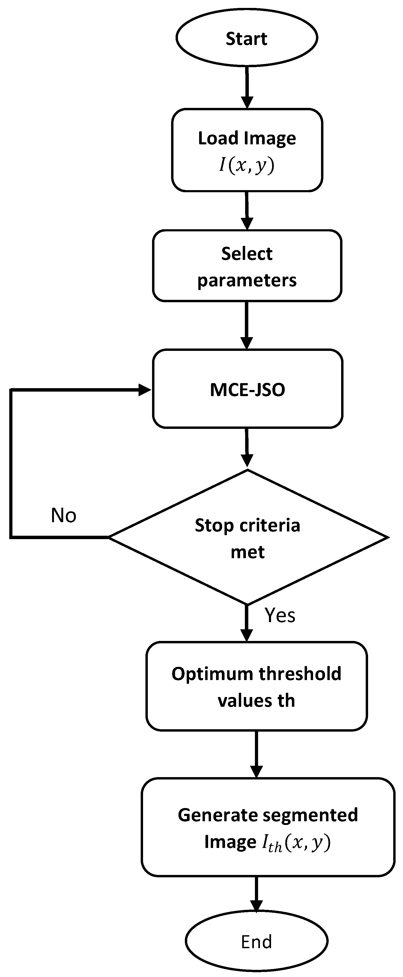
Our proposed approach focuses on the segmentation of X-ray digital images using two distinct datasets consisting of five images each, one representing healthy lungs and the other comprising X-ray digital images from lungs affected by pneumonia. In the subsequent subsections, we delve into the essential components and intricacies of our algorithm and elucidate its design and functionality in detail. A graphical description of our approach can be seen in Figure 1.

Figure 1.
MCE-JSO flow chart of proposed methodology.
- (a)
- Problem formulation
The method under consideration utilizes a multilevel thresholding technique to perform image segmentation on X-ray digital images. This method entails an analysis of pixel intensities within an image, ultimately resulting in the identification of a limited set of threshold values positioned along the energy curve. To accomplish this, we consider the capabilities of JSO algorithm to produce a variety of potential segmentation configurations. These configurations are subsequently assessed using the minimum cross-entropy (MCE) criteria to determine their effectiveness. Through a collaborative and iterative process, MCE and JSO work in tandem to pinpoint the optimal threshold values that deliver the most precise segmentation of the digital image. Essentially, the problem of minimum cross-entropy thresholding is formulated as an optimization problem, aiming to optimize the following expression:
where Equation (11), used as objective function, corresponds to the MCE formulation. The set of restrictions for the feasible space is given by the possible intensity values of a pixel encoded in an 8-bit (0–255) representation .
- (b)
- Encoding
In our methodology, we represent the threshold values by encoding them within a designated format. Each candidate solution within the population corresponds to a distinct set of these threshold values, which, in turn, dictate the division of pixel intensities in the image into various segments or categories. This encoding procedure guarantees that the thresholds are presented in a manner that allows for manipulation and optimization by the JSO algorithm.
Within the field of stochastic optimization algorithms, our approach initiates an optimization improvement process by creating an initial population of candidate solutions in a random manner. As the optimization progresses, the JSO method employs search strategies that explore positions likely to contain near-optimal or best-obtained solutions. The solutions within the population are continually updated based on information from the best solution identified during the optimization process. Once the JSO search process satisfies the predetermined termination criterion, it concludes, completing the iterative search for the optimal threshold values.
- (c)
- MCE-JSO implementation
The MCE-JSO algorithm was effectively designed to address thresholding challenges in X-ray lung digital images. The workflow is summarized as follows. Initially, the target image is loaded into memory, and its grayscale energy curve is computed. The iterative process of our approach begins with the introduction of a randomly generated population, and the solutions are progressively improved through JSO operators and a fitness function evaluation based on the MCE criteria. The procedure continues until a predefined stopping criterion is satisfied, which often involves a fixed number of generations. Finally, the optimal set of thresholds, , is employed to generate the segmented image, effectively delineating regions of interest within the X-ray image. A graphical representation of the MCE-JSO approach is shown in Figure 1.
- (d)
- Segmented image
Following the identification of an optimal set of threshold values by the JSO for a given image, , the process advances to performing multilevel thresholding, resulting in the construction of the segmented image, . The general rule governing this procedure is outlined in Equation (17). The entire methodology of our approach is effectively encapsulated in a clear and concise flowchart, as illustrated in Figure 2, providing a visual representation of the workflow of the algorithm and the sequential steps involved in the image-segmentation process.
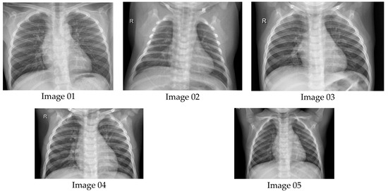
Figure 2.
Five X-rays of healthy lungs.
6. Experiments
In this section, we discuss the experiments used to assess the efficacy of our approach in segmenting pneumonia on lung radiographs. These experiments encompassed a comprehensive analysis of the mean fitness and standard deviation results, utilizing an experimental dataset comprising lung radiographs. The dataset consisted of five images representing healthy lungs and another set of images featuring pneumonia-affected lungs. The experimentation process involved two distinct phases: the initial implementation of algorithms based on histograms extracted from each digital image and, subsequently, the utilization of energy curves derived from each lung image. These experiments aimed to provide a thorough evaluation of the performance of the proposed approach in accurately segmenting pneumonia-affected regions within the radiographs.
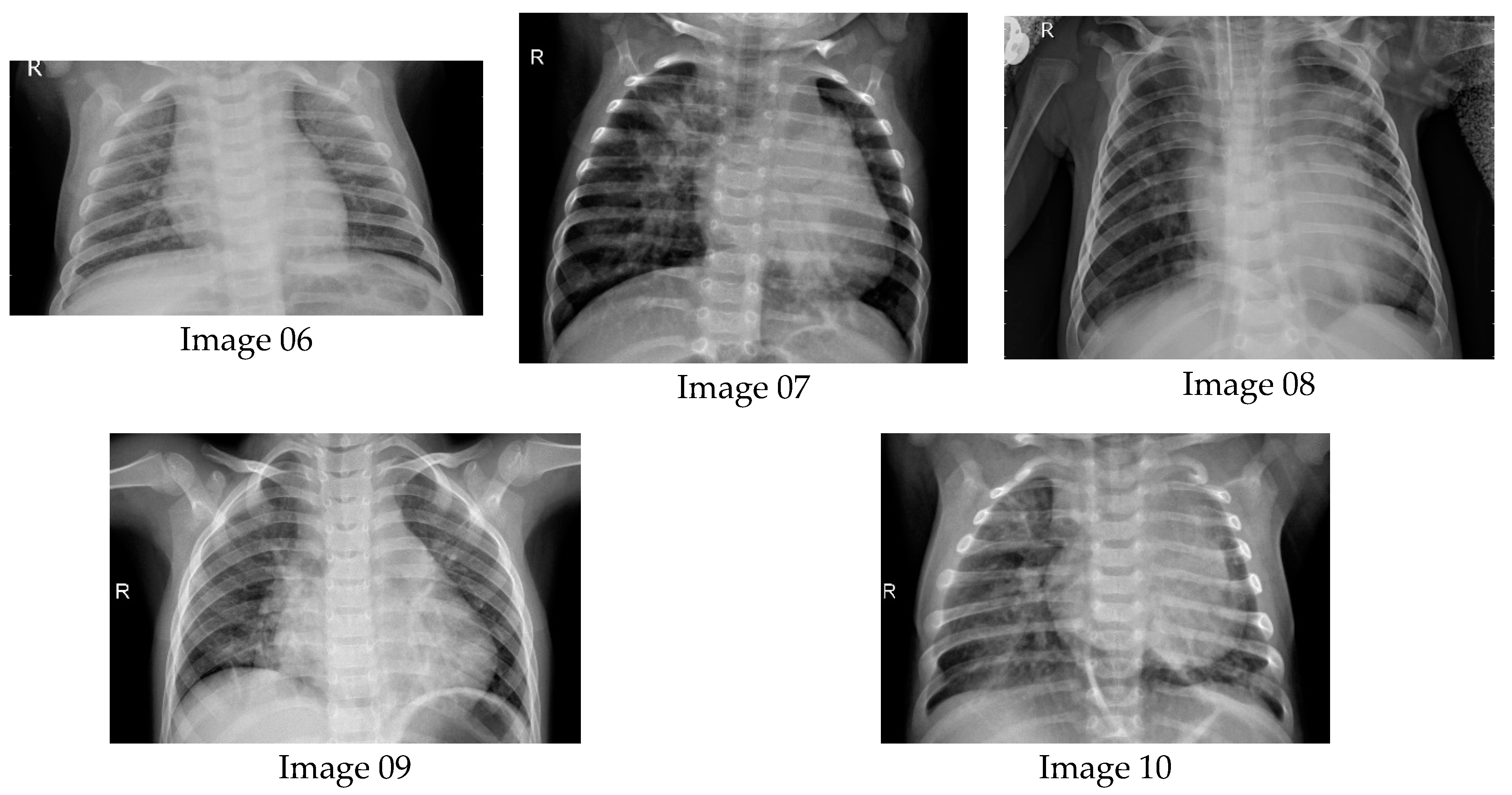
We conducted a comparative analysis of six alternative algorithms to evaluate the effectiveness of the proposed method. These experiments were performed using a dataset comprising ten digital lung images. X-ray images of healthy lungs and lungs with pneumonia are shown in Figure 2 and Figure 3, respectively.

Figure 3.
Five radiographs of lungs with pneumonia.
By systematically comparing the outcomes of our approach with those generated by existing algorithms, we aimed to provide a comprehensive assessment of the performance of the proposed method and its potential advantages in the context of segmenting lung images. The algorithms considered in the comparison were as follows:
- Levy flight distribution (LFD) [32];
- Particle swarm optimization (PSO) [33,34,35];
- Arithmetic optimization algorithm (AOA) [36,37];
- Sunflower optimization (SFO) [38,39];
- Jellyfish search optimizer (JSO) [40,41];
- Differential evolution (DE) [42,43].
In our experimental setup, all algorithms employed were configured using specific parameters, as detailed in Table 2. These parameters were selected based on the prior references of the respective algorithms, and the best performance was established. Each algorithm utilized these parameter settings to achieve optimal performance, ensuring a standardized and fair comparison of their effectiveness in the context of image segmentation. This methodology allowed us to assess the algorithms under conditions that aligned with their historically successful configurations, facilitating a meaningful evaluation of their performance against one another.

Table 2.
Parameter settings of the algorithms.
In our experimental setup, all the optimization algorithms utilized minimum cross-entropy (MCE) as the designated fitness function following the approach outlined in [26]. These metaheuristic (stochastic) algorithms employed the minimum cross-entropy criterion as their objective function while maintaining a consistent solution representation. The assessment of these methodologies relied on a range of image quality metrics including the peak signal-to-noise ratio (PSNR) [44], structural similarity index measure (SSIM) [45], and feature similarity index (FSIM) [46]. The experiments were conducted on MATLAB R2018a running on a 2.4 GHz Intel Core i5 CPU with 12 GB of RAM memory. For the experiments, we considered different threshold levels ( and values) using the minimum cross-entropy function [26] to segment digital X-Ray Images. These specific threshold values were chosen because we observed a substantial impact on algorithm performance as the number of thresholds increased, particularly for the 16 and 32 thresholds. This comprehensive evaluation aimed to provide valuable insights into the comparative performance of the algorithms across various threshold scenarios.
The experimental section of our study is divided into three distinct components, each serving a specific purpose. In the first part (Section 6.1), we present the outcomes of our proposed approach and compare its performance with those of six alternative methods. Additionally, we conducted a detailed analysis of the pivotal role of the energy curve in enhancing the performance of our algorithm. To achieve this, we draw comparisons between the results obtained using the energy curve and those obtained using a simpler histogram-based approach. The second part (Section 6.2) of our experimental analysis shifts the focus towards an in-depth assessment of the segmentation quality. Here, we employed a range of metric indices tailored to evaluate the quality of the segmented images. These metrics provide valuable insights into the precision and effectiveness of the proposed approach, offering a comprehensive evaluation of its image segmentation capabilities. Finally, the third part of our experimental section (Section 6.3) is dedicated to rigorous statistical analyses. This crucial component was designed to establish the validity and reliability of the experimental results. By subjecting our findings to statistical scrutiny, we aim to demonstrate that the observed outcomes were not the result of experimental error or chance but are indeed indicative of the inherent mechanisms and capabilities of the algorithms under examination. In essence, this multifaceted experimental approach ensures a thorough and well-rounded assessment of our proposed method for pneumonia segmentation in lung radiographs.
6.1. Results from Lung Radiographs
In this section, we evaluate the efficiency of the proposed approach using the MCE-jellyfish search algorithm. Our experiment involved a reference group of ten lung radiographs, as detailed in the dataset [47], consisting of five images from healthy lungs and five from lungs affected by pneumonia. To rigorously test the effectiveness of our approach, we employed digital images extracted from a chest X-ray images (pneumonia) dataset accessible on Kaggle, an online community of data scientists and machine learning professionals [47]. To assess and compare the performance of our method against five other optimizer algorithms, we performed digital image segmentation at seven different threshold levels: = 2, 3, 4, 5, 8, 16, and 32. This comprehensive analysis allowed us to gauge the robustness and accuracy of our proposed approach across a range of thresholding scenarios, offering valuable insights into its capabilities in the context of lung image segmentation.
The results obtained from our proposed algorithm in conjunction with the outcomes from the other six methods are presented in Table 3. The results were systematically organized considering the various thresholds employed in the segmentation process. These results unequivocally highlight the superior performance of the proposed algorithm in terms of both accuracy and robustness. In terms of accuracy, our approach consistently exhibited the lowest values of the average objective function across all threshold scenarios, surpassing the other six methods. Notably, Table 3 underscores the exceptional robustness of our algorithm, as evidenced by its minimal standard deviation values compared with the alternative methods. This lower standard deviation indicates that our algorithm consistently yielded highly consistent results, with minimal variability. By contrast, the other algorithms exhibited a broader range of values, indicating their inability to consistently deliver the same solution. These findings confirm that our algorithm consistently produced reliable results across all the threshold configurations considered in the experiments, underlining its robust and dependable performance. The competitive results achieved by the proposed approach can be attributed to two distinct and complementary elements. First, the outstanding search capabilities of the JSO algorithm play a pivotal role. This algorithm, with its capacity for systematic exploration and optimization within the solution space, effectively navigates the complex terrain of image segmentation. Second, our approach leverages an innovative energy curve, which is a crucial component. This energy curve, designed to precisely measure the elements, significantly contributes to the quality of segmentation. It not only considers pixel intensities but also incorporates spatial contextual information from the image. This comprehensive approach ensures that the elements critical for accurate segmentation are properly evaluated and utilized, ultimately leading to the robust and competitive results observed in our experiments.

Table 3.
Averaged fitness and standard deviation values for lung X-ray images using energy curve from LFD, PSO, AOA, SFO, JSO, and DE.
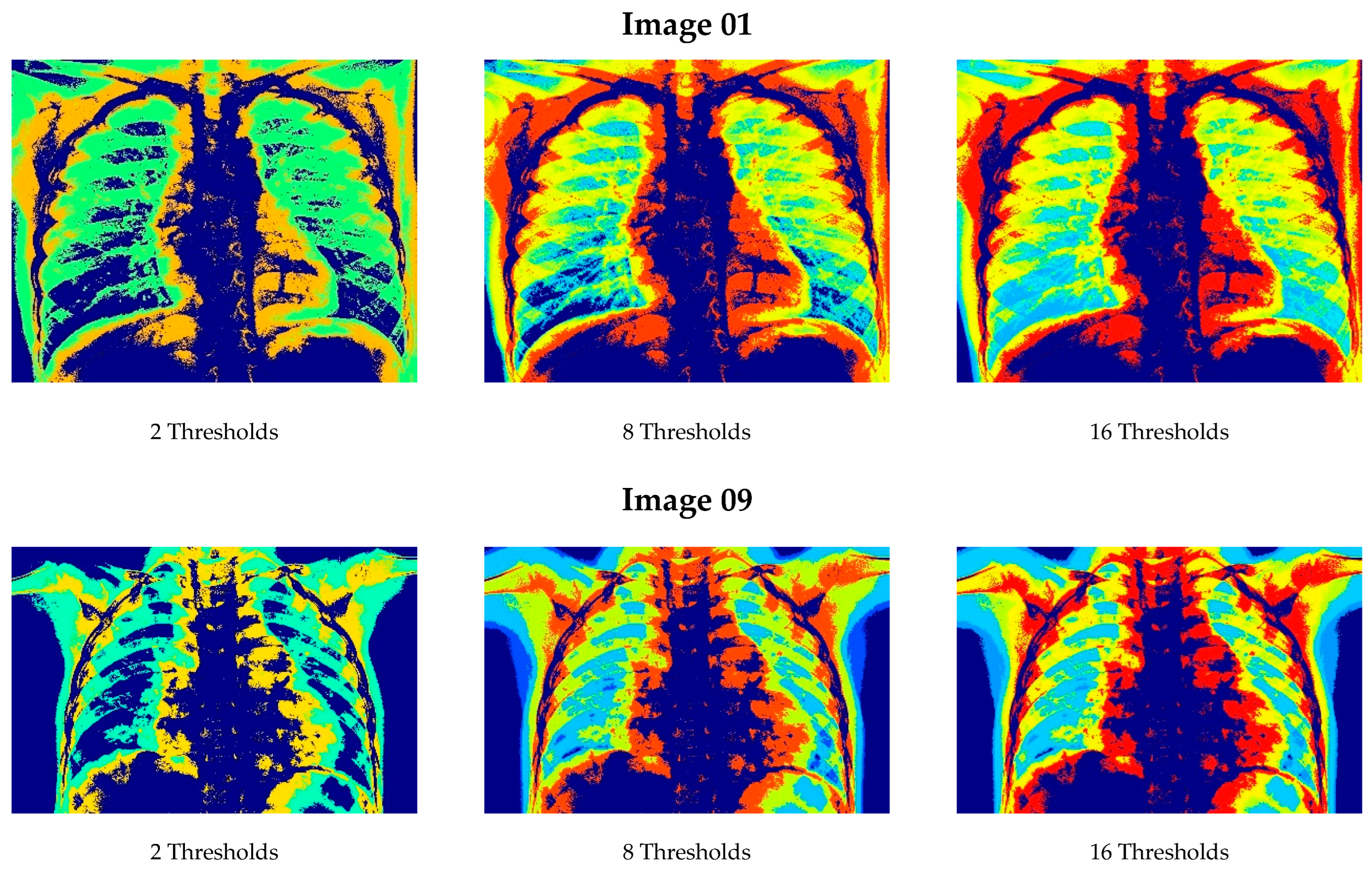
Figure 4 provides a visual representation of the segmentation outcomes achieved by the proposed approach, focusing on thresholds 2, 8, and 16 and featuring two representative images, namely, images 01 and 09. This visual showcase effectively demonstrates the performance of the algorithm in segmenting specific images. After a close examination of the images, it was evident that the proposed approach enhanced the crucial regions within the X-ray images. The segmentation results exhibited a detailed and refined delineation of the key areas, which is of paramount importance in assisting physicians with disease diagnosis. This visual evidence underscores the approach’s ability to provide precise and meaningful segmentation, contributing to more accurate medical assessments, and ultimately improving patient care.

Figure 4.
Visual results of the segmentation under the proposed method for two representative images.
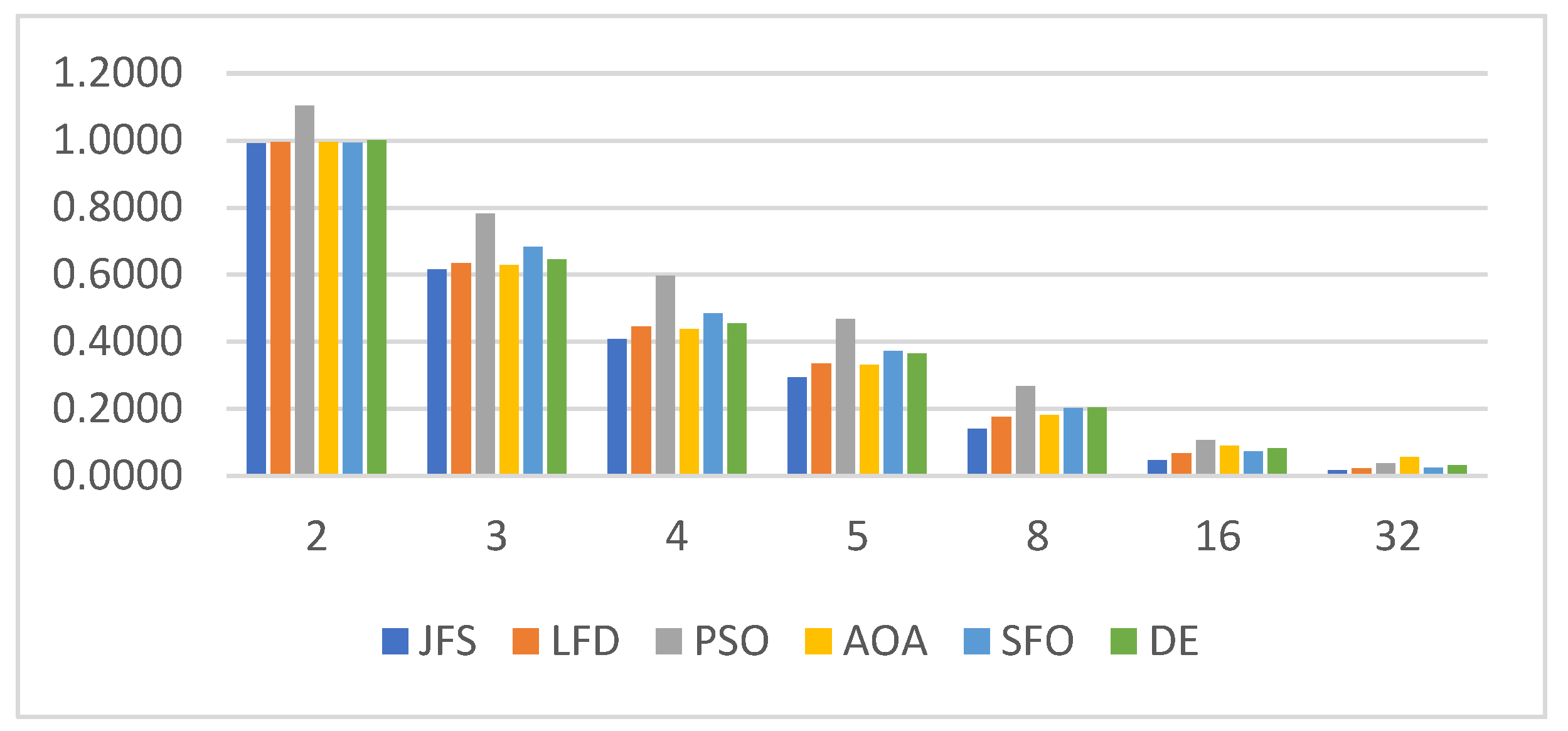
To gain a comprehensive understanding of how each algorithm performs, Figure 5 illustrates its behavior across a range of different thresholding levels. In this visualization, the performance of each algorithm was evaluated in terms of its objective function, and the results were aggregated by averaging across all the images considered in the experiments. The striking observation from this figure is the consistent superiority of the proposed algorithm, which consistently achieved the best results, as indicated by the lowest objective function values. Importantly, Figure 5 indicates that the most substantial disparities among the various methods manifested when they were tasked with segmenting images using a smaller number of thresholds, specifically, 3, 4, 5, and 8. These threshold levels are pivotal for numerous segmentation applications and clinical applications. The exceptional performance of the proposed algorithm in these critical scenarios underscores its effectiveness and reliability in accurately identifying regions of interest within the images. This visual representation provides a clear and compelling depiction of the algorithmic performance across the different thresholding levels, reinforcing the outstanding capabilities of the proposed approach in image segmentation tasks.
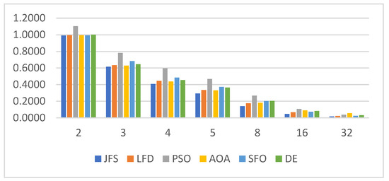
Figure 5.
Performance comparison among the methods considering energy curve.
To investigate the impact of the energy curve on the segmentation outcomes, we conducted an additional experiment in which the energy curve was replaced by a conventional histogram. The aim of this experiment was to demonstrate the superior performance achieved by using the energy curve. The results of this experiment are presented in Table 4, where it is evident that the values obtained by all the algorithms were generally higher than those reported in Table 3. This shift indicates that the utilization of the energy curve led to solutions that penalized less important elements, consequently highlighting the most critical areas within the X-ray image. As such, it can be deduced that the incorporation of the energy curve is a pivotal factor in achieving competitive results and, more importantly, in assisting physicians in the accurate detection of pneumonia. The ability of the energy curve to consider both the intensity and spatial information elevates its significance in image segmentation tasks, as evidenced by the contrasting results between the two experiments.

Table 4.
Averaged fitness and standard deviation values for lung X-ray images using histogram from LFD, PSO, AOA, SFO, JSO, and DE.
To compare the impact of utilizing the energy curve against the conventional histogram in the objective function, Figure 6 provides a comprehensive comparison. This figure highlights the outcomes of the cost function minimization for the proposed algorithm (JSO method), with the results averaged across the 10 images employed in the experiment. The key observation from this illustration is the discernible difference in the performance between the two approaches.
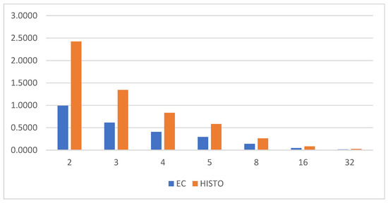
Figure 6.
Comparative results of the energy curve vs. histogram under the JSO.
As depicted in the image, the use of the energy curve consistently yielded superior results compared to the use of the histogram, particularly at thresholds 2, 3, 4, and 5. These specific threshold levels are critical in image segmentation tasks because they often correspond to essential regions of interest. The clear contrast in performance underscores the efficacy of incorporating the energy curve, as it led to more accurate and meaningful segmentation results. This visual representation provides compelling evidence of the advantages offered by the energy curve in enhancing the performance of the algorithm, particularly in scenarios in which precise segmentation is paramount.
6.2. Evaluating Segmentation Quality
The assessment of image segmentation results requires an evaluation of various quality indices to provide an objective measure of performance. In this study, we employed a set of well-established metrics to evaluate the quality of segmented images. These metrics included the peak signal-to-noise ratio (PSNR), structural similarity index method (SSIM), and feature similarity index method (FSIM). These indexes were chosen for their ability to objectively and quantitatively assess the quality of the segmentation outcomes. Using these metrics, we could effectively gauge the accuracy and fidelity of the segmented images, providing a robust and objective basis for evaluating the performance of segmentation algorithms.
- (A)
- Peak Signal-To-Noise Ratio (PSNR)
The peak signal-to-noise ratio (PSNR) [44] is a widely used metric for evaluating the quality of segmented images. It quantifies the level of noise or distortion present in a segmented image by comparing it to the original unsegmented image. A higher PSNR value indicates a lower level of distortion or error, which implies that the segmented image closely resembles the original image. In essence, the PSNR provides a quantitative measure of how faithfully the segmentation process preserves the details and information of the image. This metric is particularly valuable for assessing the accuracy and fidelity of segmentation results, making it an essential tool for image analysis and processing tasks. The PSNR is computed as follows:
Figure 7 provides a visual representation of the peak signal-to-noise ratio (PSNR) results, offering valuable insights into the quality of the segmented images. These PSNR values were obtained by averaging the index over the ten images utilized in the experiments, resulting in a comprehensive assessment of the performance. This figure shows several important observations. First, when considering the two thresholds, the results of all algorithms appeared similar, indicating comparable performance in this specific scenario. However, the most significant disparities became evident when examining the outcomes for the 8, 16, and 32 thresholds. In these cases, the proposed approach consistently outperformed its competitors, exhibiting markedly higher PSNR values. This observation underscores the effectiveness of our approach in preserving image quality and minimizing distortion during the segmentation process. The superior PSNR values for the higher threshold configurations reaffirm the capability of the algorithm to deliver accurate and high-quality segmented images, which is a critical factor in medical image analysis and diagnosis. From these results, it can be seen that our method obtained a better PSNR value for the case of the 32 levels, which on average was 15%.
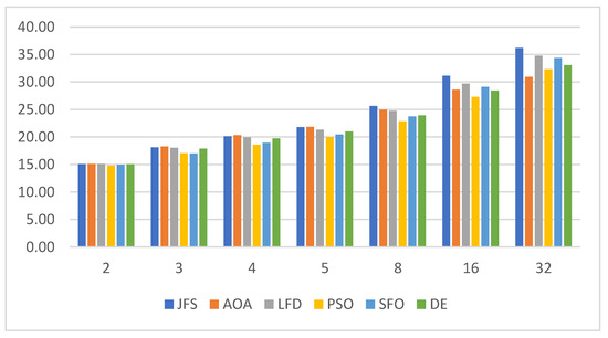
Figure 7.
Comparative analysis in terms of .
- (B)
- Structural Similarity Index Method (SSIM)
The structural similarity index method (SSIM) [45] is a robust metric used to assess the quality of segmented images. It measures the structural similarity between a segmented image and a reference image, often the original unsegmented image. The SSIM considers various factors, including luminance, contrast, and structure, to evaluate how well the segmented image preserves the important structural information present in the reference image. A higher SSIM score indicates a closer resemblance between the segmented and reference images, implying a better segmentation quality. The SSIM provides a holistic assessment of both local and global structural similarities, making it a valuable tool for objectively evaluating the accuracy and fidelity of segmented images. The SSIM is computed as follows:
where and are the mean values of the original and the segmented image, respectively, where for each image, the values of and correspond to the standard deviation. and are constants used to avoid instability when , both values of which in this experiment were
Figure 8 visually presents the results of the structural similarity index method (SSIM) index, providing an insightful assessment of the quality of the segmented images. These SSIM values represent the average index across the ten images involved in the experiments, offering a comprehensive evaluation of the performance. This figure presents several noteworthy observations.

Figure 8.
Comparative analysis in terms of
Initially, when considering scenarios with only two thresholds, the results of all the algorithms appeared uniform, indicating similar performance levels in this particular context. However, significant disparities emerged when evaluating the outcomes for the 8, 16, and 32 thresholds. In these cases, the proposed approach consistently outperformed its competitors and demonstrated substantially higher SSIM values. This underscores the proficiency of the algorithm in preserving both the local and global structural similarities between the segmented and reference images. The superior SSIM values for the higher-threshold configurations reaffirm the effectiveness of the proposed approach in delivering accurate and high-quality segmented images, which is crucial for applications in medical image analysis and diagnosis. From these results, it can be seen that our method obtained a better value of the SSIM for the case of the 32 levels, which on average was 8%.
- (C)
- Feature Similarity Index Method (FSIM)
The feature similarity index method (FSIM) [46] is employed to evaluate the quality of segmented images. The FSIM focuses on assessing the quality of structural and textural information in a segmented image by comparing it to a reference image, typically the original unsegmented image. Unlike traditional metrics that consider luminance and structural factors, the FSIM places strong emphasis on capturing the perceptual quality of a segmented image. It analyzes features, such as edges, textures, and patterns, to determine how faithfully these essential aspects are preserved during the segmentation process. A higher FSIM score signifies closer similarity between the segmented and reference images, reflecting better segmentation quality in terms of preserving critical visual features and textures. The FSIM is particularly valuable for evaluating the perceptual quality of segmented images, making it a crucial tool for various image analysis applications. The FSIM index is computed as follows:
where Ω denotes the domain of the image.
Figure 9 illustrates the outcomes of the feature similarity index method (FSIM) applied to segmented lung X-ray images generated by each of the six algorithms. This presentation offers valuable insights into the perceptual quality of the segmented images. In the case of the FSIM test, there was a notable consistency in the results produced by each optimization algorithm, particularly when considering the scenarios with lower threshold counts. However, a striking contrast emerged when the number of thresholds increased. In these instances, the proposed algorithm consistently exhibited superior results, with FSIM scores approaching the maximum value of 1. This observation emphasizes the effectiveness of the algorithm in preserving essential visual features, textures, and patterns within segmented images, even when faced with the challenges posed by higher-threshold configurations. The close proximity of the results of the proposed algorithm to the maximum FSIM value underscores its capacity to deliver perceptually high-quality segmented images, which is of paramount importance in medical image analysis and clinical diagnosis. From these results, it can be seen that our method obtained a better FSIM value for the case of the 32 levels, which on average was 6%.
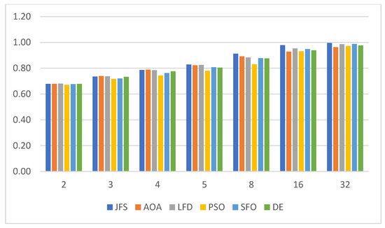
Figure 9.
Comparative analysis in terms of .
6.3. Statistical Analysis
The primary objective of the statistical analysis in this study was to establish that the superior results achieved by the proposed algorithm in comparison to the other methods were attributable to the algorithm’s inherent capabilities rather than random chance or experimental variability. To address this objective rigorously, we employed the Kruskal–Wallis test [48].
The Kruskal–Wallis test is a non-parametric statistical test used to assess whether there are significant differences between three or more independent groups. It is often employed when the data do not meet the assumptions of the normal distribution or homogeneity of variances required for parametric tests such as analysis of variance (ANOVA) [49].
In our comprehensive analysis, data were collected from a series of experiments, each comprising thirty independent runs for each of the six algorithms under evaluation. These experiments encompassed a wide range of threshold values, including 2, 3, 4, 5, 8, 16, and 32 thresholds, ensuring a thorough assessment of the algorithm performance across the various configurations. To determine the statistical significance of the observed results, we established a predefined significance level denoted as α. This value played a crucial role in the hypothesis testing process. The hypothesis under consideration was the null hypothesis (), which posits that there were no significant differences among the algorithms, implying that the observed variations were merely due to chance or randomness. To ascertain whether we can reject this null hypothesis, we conducted a Kruskal–Wallis test and compared its output with . If the test yielded a -value lower than , it signified that the algorithms exhibited statistically significant differences in their performances. This outcome empowered us to conclude that the variations in the results were not mere chance occurrences but rather reflect genuine distinctions in the capabilities of the evaluated algorithms. This rigorous statistical approach ensured the validity and reliability of the comparative analyses.
Based on the comprehensive statistical analysis, a robust conclusion was drawn regarding the performance of the proposed method in comparison with the other algorithms. These findings unequivocally established that the superior results achieved by the proposed method were not a consequence of experimental error or random variability. Instead, they were attributed to the inherent capabilities and efficacy of the proposed algorithm.
To gain a deeper understanding of the statistical results that elucidate the performance of the proposed approach, Figure 10 provides a comprehensive visual representation through a box plot. This graphical presentation offers an insightful depiction of each algorithm’s performance, featuring central tendencies (visualized as red lines) denoting the average results and the dispersion represented by the width of the box. After close examination of the figure, a compelling pattern emerged. The proposed algorithm conspicuously stands out as the method with the lowest average value compared with the other methods. This signifies that on average, the proposed method consistently outperformed its counterparts, offering superior solutions to the segmentation problem at hand. A noteworthy observation relates to the dispersion of the results among the methods. Although the other methods exhibited a considerable spread in their outcomes, indicating substantial variability in terms of performance, the proposed method distinguished itself by consistently yielding results with minimal dispersion. In other words, the proposed algorithm consistently provided results that were closely clustered, underscoring its remarkable stability and reliability. In summary, Figure 10 provides a compelling visual testament to the exceptional performance and robustness of the proposed approach, highlighting its capacity to consistently deliver superior solutions while maintaining a high degree of result consistency, which is a crucial attribute in the realms of optimization and image segmentation.
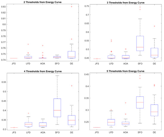

Figure 10.
Statistical results of averaged values and dispersion through a box plot.
7. Conclusions
In this study, we introduced a novel and highly effective segmentation method designed for the precise identification of pneumonia on lung radiographs. Our approach uses the JSO, a metaheuristic algorithm renowned for its exceptional global exploration capabilities and robust performance. The core of our methodology is the utilization of an energy curve as the cost function, which hinged upon the principles of cross-entropy. This energy curve plays a pivotal role in enhancing segmentation accuracy by imposing heavier penalties on misclassified pixels, thus directing the algorithm’s attention towards regions where segmentation errors are most likely to occur. The strategic application of this energy-based cross-entropy cost function is of paramount importance, as it ensures the precise delineation of objects or regions of interest within radiographs—a critical requirement for the accurate diagnosis and monitoring of pneumonia. Our approach not only demonstrates the capacities of JSO but also underscores the significance of advanced cost functions in the area of medical image segmentation.
To validate the proposed approach, a comprehensive assessment was conducted using a diverse dataset of X-ray images sourced from both healthy individuals and patients with pneumonia. In these experiments, our MCE-JSO method was subjected to a thorough comparative analysis of several alternative stochastic optimization techniques. The algorithms used in the comparison included levy flight distribution (LFD), particle swarm optimization (PSO), the arithmetic optimization algorithm (AOA), sunflower optimization (SFO), and differential evolution (DE). The evaluation process revolved around an in-depth examination of the quality of image segmentation achieved through these algorithms. To evaluate the performance objectively, we employed key image quality metrics, such as the peak signal-to-noise ratio (PSNR), structural similarity index measure (SSIM), and feature similarity index. These metrics provided a robust quantitative assessment of the segmentation results, allowing us to discern the nuances in algorithm performance. To ensure the robustness and reliability of our findings, the results were subjected to statistical scrutiny, encompassing multiple tests and analyses. This multifaceted approach to validation not only reaffirmed the effectiveness of our proposed method but also offered a comprehensive and data-driven evaluation of its performance in the context of pneumonia detection in X-ray images.
We conducted a dedicated experiment to expand our analysis and to elucidate the pivotal role of the energy curve in the segmentation process. This experiment served as a crucial means to highlight the significance of our chosen approach compared to a more straightforward method using a simple histogram.
The exceptional performance achieved by our proposed approach can be attributed to the synergy between the two distinct yet highly complementary elements. First, the JSO algorithm takes the spotlight owing to its remarkable search capabilities. With its systematic and exhaustive exploration of the solution space, JSO effectively navigates the intricate landscape of image segmentation and optimizes the process with precision. Second, our approach strategically incorporates an innovative energy curve, which is a critical component that significantly enhances segmentation quality. Unlike traditional methods that rely solely on pixel intensities, this energy curve goes a step further by incorporating the spatial contextual information of an image. Considering these spatial nuances, the curve ensures that elements crucial for accurate segmentation are meticulously evaluated and leveraged. This comprehensive and holistic approach, encompassing both advanced search capabilities and the energy curve, synergizes to produce the robust and competitive results observed in our experiments.
Author Contributions
Software, O.Z.; Validation, O.Z.; Formal analysis, D.Z.; Investigation, E.C. and M.P. All authors have read and agreed to the published version of the manuscript.
Funding
This research was funded by SICyT-Jalisco and COECYTJAL , FODECYTJAL 2022, DISEÑO DE NUEVOS VEHÍCULOS SUSTENTABLES E INTELIGENTES EN JALISCO grant number 10300.
 , FODECYTJAL 2022, DISEÑO DE NUEVOS VEHÍCULOS SUSTENTABLES E INTELIGENTES EN JALISCO grant number 10300.
Data Availability Statement
Not applicable.
Conflicts of Interest
The authors declare no conflict of interest.
References
- Gao, C.A.; Markov, N.S.; Stoeger, T.; Pawlowski, A.E.; Kang, M.; Nannapaneni, P.; Grant, R.A.; Pickens, C.; Walter, J.M.; Kruser, J.M.; et al. Machine learning links unresolving secondary pneumonia to mortality in patients with severe pneumonia, including COVID-19. J. Clin. Investig. 2023, 133, e170682. [Google Scholar] [CrossRef]
- Abdullah, S.H.; Abedi, W.M.S.; Hadi, R.M. Enhanced feature selection algorithm for pneumonia detection. Period. Eng. Nat. Sci. 2023, 10, 168–180. [Google Scholar] [CrossRef]
- Xie, P.; Zhao, X.; He, X. Improve the performance of CT-based pneumonia classification via source data reweighting. Sci. Rep. 2023, 13, 9401. [Google Scholar] [CrossRef] [PubMed]
- Yan, N.; Tao, Y. Pneumonia X-ray detection with anchor-free detection framework and data augmentation. Int. J. Imaging Syst. Technol. 2023, 33, 1235–1246. [Google Scholar] [CrossRef]
- Asswin, C.R.; KS, D.K.; Dora, A.; Ravi, V.; Sowmya, V.; Gopalakrishnan, E.A.; Soman, K.P. Transfer learning approach for pediatric pneumonia diagnosis using channel attention deep CNN architectures. Eng. Appl. Artif. Intell. 2023, 123, 106416. [Google Scholar]
- Kaya, Y.; Gürsoy, E. A MobileNet-based CNN model with a novel fine-tuning mechanism for COVID-19 infection detection. Soft Comput. 2023, 27, 5521–5535. [Google Scholar] [CrossRef] [PubMed]
- Chen, S.; Ren, S.; Wang, G.; Huang, M.; Xue, C. Interpretable CNN-Multilevel Attention Transformer for Rapid Recognition of Pneumonia from Chest X-ray Images. IEEE J. Biomed. Health Inform. 2023; online ahead of print. [Google Scholar]
- Sanghvi, H.A.; Patel, R.H.; Agarwal, A.; Gupta, S.; Sawhney, V.; Pandya, A.S. A deep learning approach for classification of COVID and pneumonia using DenseNet-201. Int. J. Imaging Syst. Technol. 2023, 33, 18–38. [Google Scholar] [CrossRef]
- AnbuDevi, M.K.A.; Suganthi, K. Review of Semantic Segmentation of Medical Images Using Modified Architectures of UNET. Diagnostics 2022, 12, 3064. [Google Scholar] [CrossRef]
- Zhou, Z.; Siddiquee, M.M.R.; Tajbakhsh, N.; Liang, J. Unet++: Redesigning skip connections to exploit multiscale features in image segmentation. IEEE Trans. Med. Imaging 2019, 39, 1856–1867. [Google Scholar] [CrossRef]
- Diakogiannis, F.I.; Waldner, F.; Caccetta, P.; Wu, C. ResUNet-a: A deep learning framework for semantic segmentation of remotely sensed data. ISPRS J. Photogramm. Remote Sens. 2020, 162, 94–114. [Google Scholar] [CrossRef]
- Li, X.; Chen, H.; Qi, X.; Dou, Q.; Fu, C.W.; Heng, P.A. H-DenseUNet: Hybrid densely connected UNet for liver and tumor segmentation from CT volumes. IEEE Trans. Med. Imaging 2018, 37, 2663–2674. [Google Scholar] [CrossRef] [PubMed]
- Aiadi, O.; Khaldi, B. A fast lightweight network for the discrimination of COVID-19 and pulmonary diseases. Biomed. Signal Process. Control 2022, 78, 103925. [Google Scholar] [CrossRef]
- Basu, A.; Sheikh, K.H.; Cuevas, E.; Sarkar, R. COVID-19 detection from CT scans using a two-stage framework. Expert Syst. Appl. 2022, 193, 116377. [Google Scholar] [CrossRef]
- Xue, X.; Chinnaperumal, S.; Abdulsahib, G.M.; Manyam, R.R.; Marappan, R.; Raju, S.K.; Khalaf, O.I. Design and Analysis of a Deep Learning Ensemble Framework Model for the Detection of COVID-19 and Pneumonia Using Large-Scale CT Scan and X-ray Image Datasets. Bioengineering 2023, 10, 363. [Google Scholar] [CrossRef] [PubMed]
- Issa, M.; Helmi, A.M.; Elsheikh, A.H.; Abd Elaziz, M. A biological sub-sequences detection using integrated BA-PSO based on infection propagation mechanism: Case study COVID-19. Expert Syst. Appl. 2022, 189, 116063. [Google Scholar] [CrossRef] [PubMed]
- Abualigah, L.; Diabat, A.; Sumari, P.; Gandomi, A.H. A novel evolutionary arithmetic optimization algorithm for multilevel thresholding segmentation of COVID-19 ct images. Processes 2021, 9, 1155. [Google Scholar] [CrossRef]
- Kumar, N.M.; Premalatha, K.; Suvitha, S. Lung disease detection using Self-Attention Generative Adversarial Capsule network optimized with sun flower Optimization Algorithm. Biomed. Signal Process. Control 2023, 79, 104241. [Google Scholar]
- Singh, D.; Kumar, V.; Vaishali; Kaur, M. Classification of COVID-19 patients from chest CT images using multi-objective differential evolution–based convolutional neural networks. Eur. J. Clin. Microbiol. Infect. Dis. 2020, 39, 1379–1389. [Google Scholar] [CrossRef]
- Chou, J.-S.; Ngo, N.-T. Modified firefly algorithm for multidimensional optimization in structural design problems. Struct. Multidiscip. Optim. 2017, 55, 2013–2028. [Google Scholar] [CrossRef]
- Shaheen, A.M.; El-Sehiemy, R.A.; Alharthi, M.M.; Ghoneim, S.S.; Ginidi, A.R. Multi-objective jellyfish search optimizer for efficient power system operation based on multi-dimensional OPF framework. Energy 2021, 237, 121478. [Google Scholar] [CrossRef]
- Kaveh, A.; Biabani Hamedani, K.; Kamalinejad, M.; Joudaki, A. Quantum-based jellyfish search optimizer for structural optimization. Int. J. Optim. Civil. Eng. 2021, 11, 329–356. [Google Scholar]
- Farhat, M.; Kamel, S.; Atallah, A.M.; Khan, B. Optimal power flow solution based on jellyfish search optimization considering uncertainty of renewable energy sources. IEEE Access 2021, 9, 100911–100933. [Google Scholar] [CrossRef]
- Oliva, D.; Hinojosa, S.; Osuna-Enciso, V.; Cuevas, E.; Pérez-Cisneros, M.; Sanchez-Ante, G. Image segmentation by minimum cross entropy using evolutionary methods. Soft Comput. 2019, 23, 431–450. [Google Scholar] [CrossRef]
- Kullback, S. Information Theory and Statistics; Courier Corporation: Chelmsford, MA, USA, 1997. [Google Scholar]
- Li, C.H.; Lee, C.K. Minimum cross entropy thresholding. Pattern Recognit. 1993, 26, 617–625. [Google Scholar] [CrossRef]
- Hammouche, K.; Diaf, M.; Siarry, P. A comparative study of various meta-heuristic techniques applied to the multilevel thresholding problem. Eng. Appl. Artif. Intell. 2010, 23, 676–688. [Google Scholar] [CrossRef]
- Sankur, B.; Sezgin, M. Survey over image thresholding techniques and quantitative performance evaluation. J. Electron. Imaging 2004, 13, 146–168. [Google Scholar] [CrossRef]
- Ghosh, S.; Bruzzone, L.; Patra, S.; Bovolo, F.; Ghosh, A. A contextsensitive technique for unsupervised change detection based on hopfield hopfieldtype neural networks. IEEE Trans. Geosci. Remote. Sens. 2007, 45, 778–789. [Google Scholar] [CrossRef]
- Patra, S.; Gautam, R.; Singla, A. A novel context sensitive multilevel thresholding for image segmentation. Appl. Soft Comput. 2014, 23, 122–127. [Google Scholar] [CrossRef]
- Oliva, D.; Hinojosa, S.; Abd Elaziz, M.; Ortega-Sánchez, N. Context based image segmentation using antlion optimization and sine cosine algorithm. Multimed. Tools Appl. 2018, 77, 25761–25797. [Google Scholar] [CrossRef]
- Houssein, E.H.; Saad, M.R.; Hashim, F.A.; Shaban, H.; Hassaballah, M. L′evy flight distribution: A new metaheuristic algorithm for solving engineering optimization problems. Eng. Appl. Artif. Intell. 2020, 94, 103731. [Google Scholar] [CrossRef]
- Kennedy, J.; Eberhart, R. Particle swarm optimization. In Proceedings of the ICNN’95-International Conference on Neural Networks, Perth, WA, Australia, 27 November–1 December 1995; IEEE: Piscataway, NJ, USA, 1995; Volume 4, pp. 1942–1948. [Google Scholar]
- Maitra, M.; Chatterjee, A. A hybrid cooperative–comprehensive learning based pso algorithm for image segmentation using multilevel thresholding. Expert Syst. Appl. 2008, 34, 1341–1350. [Google Scholar] [CrossRef]
- Xiang, T.; Liao, X.; Wong, K.-W. An improved particle swarm optimization algorithm combined with piecewise linear chaotic map. Appl. Math. Comput. 2007, 190, 1637–1645. [Google Scholar] [CrossRef]
- Abualigah, L.; Diabat, A.; Mirjalili, S.; Abd Elaziz, M.; Gandomi, A.H. The arithmetic optimization algorithm. Comput. Methods Appl. Mech. Eng. 2021, 376, 113609. [Google Scholar] [CrossRef]
- Khatir, S.; Tiachacht, S.; Le Thanh, C.; Ghandourah, E.; Mirjalili, S.; Wahab, M.A. An improved artificial neural network using arithmetic optimization algorithm for damage assessment in fgm composite plates. Compos. Struct. 2021, 273, 114287. [Google Scholar] [CrossRef]
- Gomes, G.F.; da Cunha, S.S., Jr.; Ancelotti, A.C. A sunflower optimization (sfo) algorithm applied to damage identification on laminated composite plates. Eng. Comput. 2019, 35, 619–626. [Google Scholar] [CrossRef]
- Yuan, Z.; Wang, W.; Wang, H.; Razmjooy, N. A new technique for optimal estimation of the circuit-based pemfcs using developed sunflower optimization algorithm. Energy Rep. 2020, 6, 662–671. [Google Scholar] [CrossRef]
- Chou, J.-S.; Truong, D.-N. A novel metaheuristic optimizer inspired by behavior of jellyfish in ocean. Appl. Math. Comput. 2021, 389, 125535. [Google Scholar] [CrossRef]
- Fossette, S.; Gleiss, A.C.; Chalumeau, J.; Bastian, T.; Armstrong, C.D.; Vandenabeele, S.; Karpytchev, M.; Hays, G.C. Current-oriented swimming by jellyfish and its role in bloom maintenance. Curr. Biol. 2015, 25, 342–347. [Google Scholar] [CrossRef]
- Storn, R.; Price, K. Differential evolution—A simple and efficient heuristic for global optimization over continuous spaces. J. Glob. Optim. 1997, 11, 341–359. [Google Scholar] [CrossRef]
- Cuevas, E.; Zaldivar, D.; Pérez-Cisneros, M. A novel multi-threshold segmentation approach based on differential evolution optimization. Expert Syst. Appl. 2010, 37, 5265–5271. [Google Scholar] [CrossRef]
- Avcibas, I.; Sankur, B.; Sayood, K. Statistical evaluation of image quality measures. J. Electron. Imaging 2002, 11, 206–223. [Google Scholar]
- Wang, Z.; Bovik, A.C.; Sheikh, H.R.; Simoncelli, E.P. Image quality assessment: From error visibility to structural similarity. IEEE Trans. Image Process. 2004, 13, 600–612. [Google Scholar] [CrossRef]
- Zhang, L.; Zhang, L.; Mou, X.; Zhang, D. FSIM: A feature similarity index for image quality assessment. IEEE Trans. Image Process. 2011, 20, 2378–2386. [Google Scholar] [CrossRef] [PubMed]
- Kaggle. Chest X-ray Images (Pneumonia). 10 February 2018. Available online: https://www.kaggle.com/datasets/paultimothymooney/chest-xray-pneumonia (accessed on 24 August 2023).
- Theodorsson-Norheim, E. Kruskal-wallis test: Basic computer program to perform nonparametric one-way analysis of variance and multiple comparisons on ranks of several independent samples. Comput. Methods Programs Biomed. 1986, 23, 57–62. [Google Scholar] [CrossRef] [PubMed]
- Scheffe, H. The Analysis of Variance; John Wiley & Sons: Hoboken, NJ, USA, 1999; Volume 72. [Google Scholar]
Disclaimer/Publisher’s Note: The statements, opinions and data contained in all publications are solely those of the individual author(s) and contributor(s) and not of MDPI and/or the editor(s). MDPI and/or the editor(s) disclaim responsibility for any injury to people or property resulting from any ideas, methods, instructions or products referred to in the content. |
© 2023 by the authors. Licensee MDPI, Basel, Switzerland. This article is an open access article distributed under the terms and conditions of the Creative Commons Attribution (CC BY) license (https://creativecommons.org/licenses/by/4.0/).

