
Enhancing Pneumonia Segmentation in Lung Radiographs: A Jellyfish Search Optimizer Approach

Abstract
:1. Introduction
2. Jellyfish Search Optimizer (JSO)
3. Image Segmentation with Minimum Cross-Entropy
4. Energy Curve
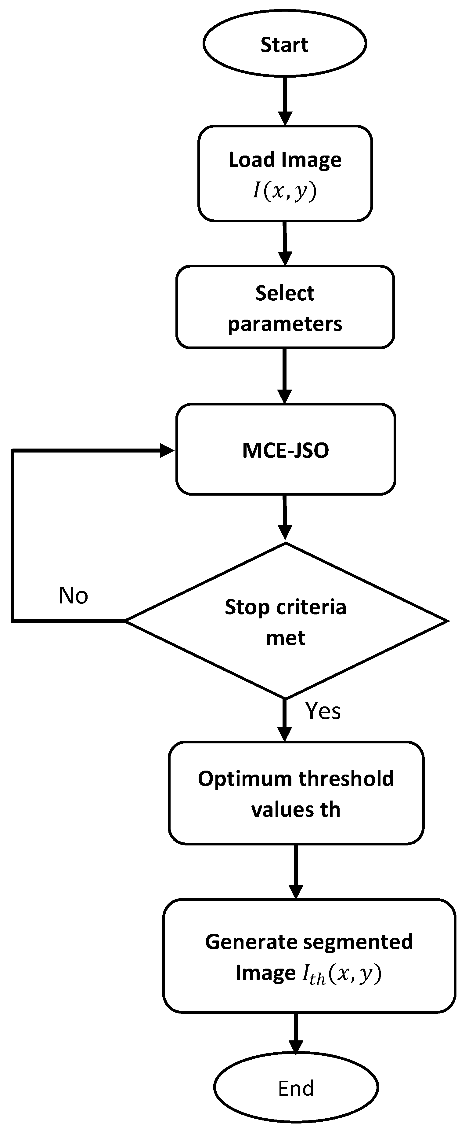
5. Proposed Method
- (a)
- Problem formulation
- (b)
- Encoding
- (c)
- MCE-JSO implementation
- (d)
- Segmented image
6. Experiments
- Levy flight distribution (LFD) [32];
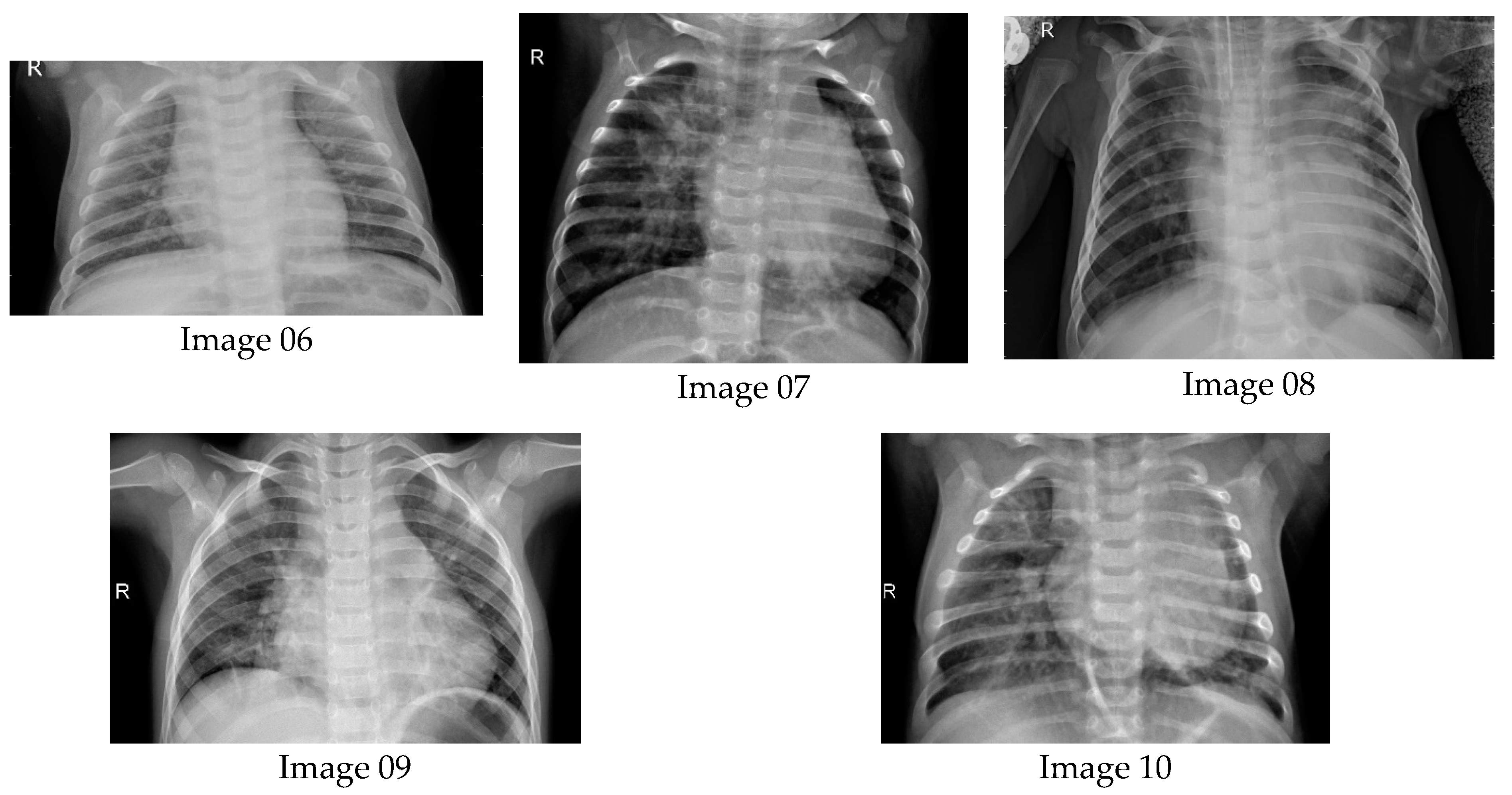
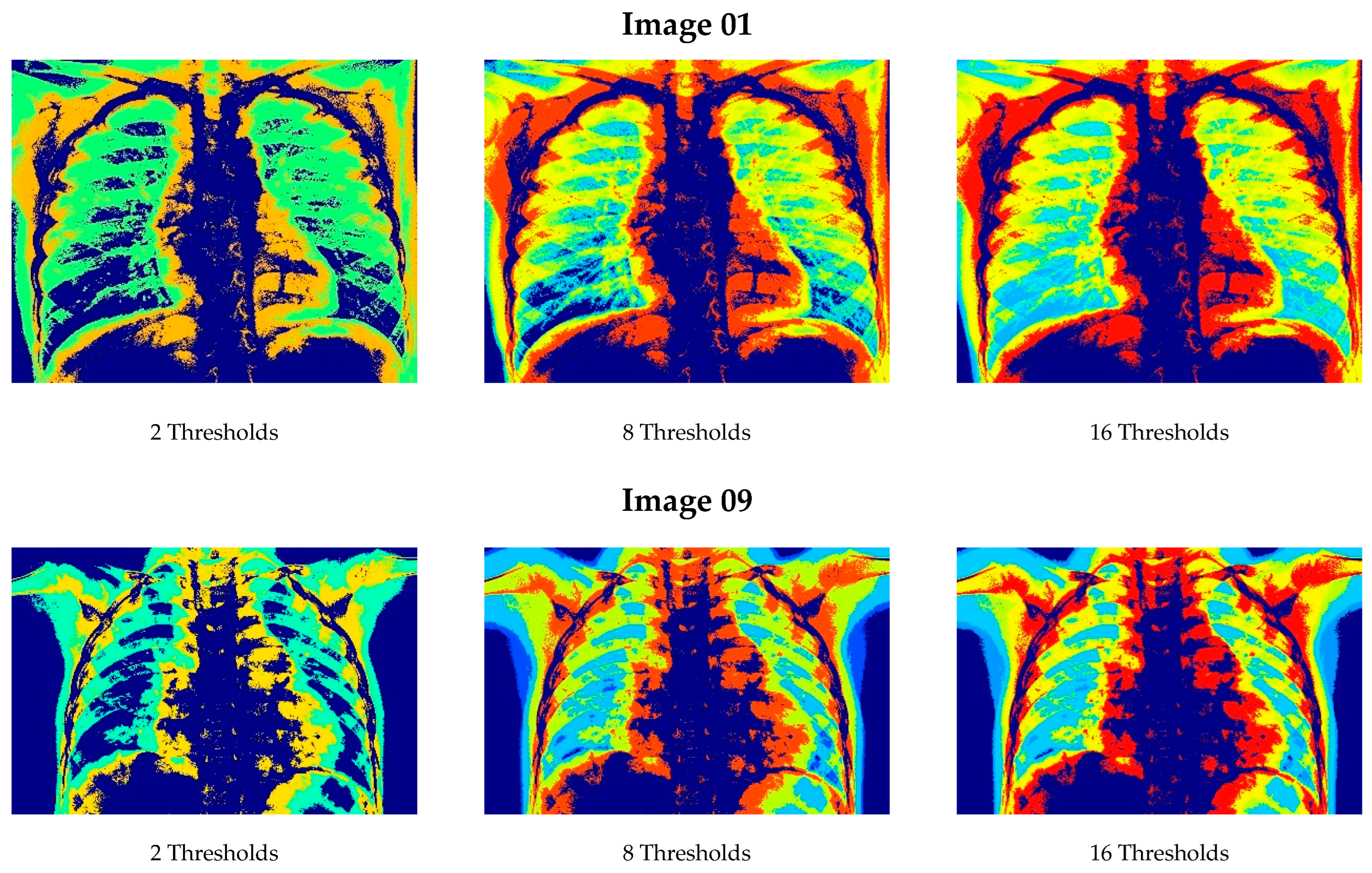
6.1. Results from Lung Radiographs
6.2. Evaluating Segmentation Quality
- (A)
- Peak Signal-To-Noise Ratio (PSNR)
- (B)
- Structural Similarity Index Method (SSIM)
- (C)
- Feature Similarity Index Method (FSIM)
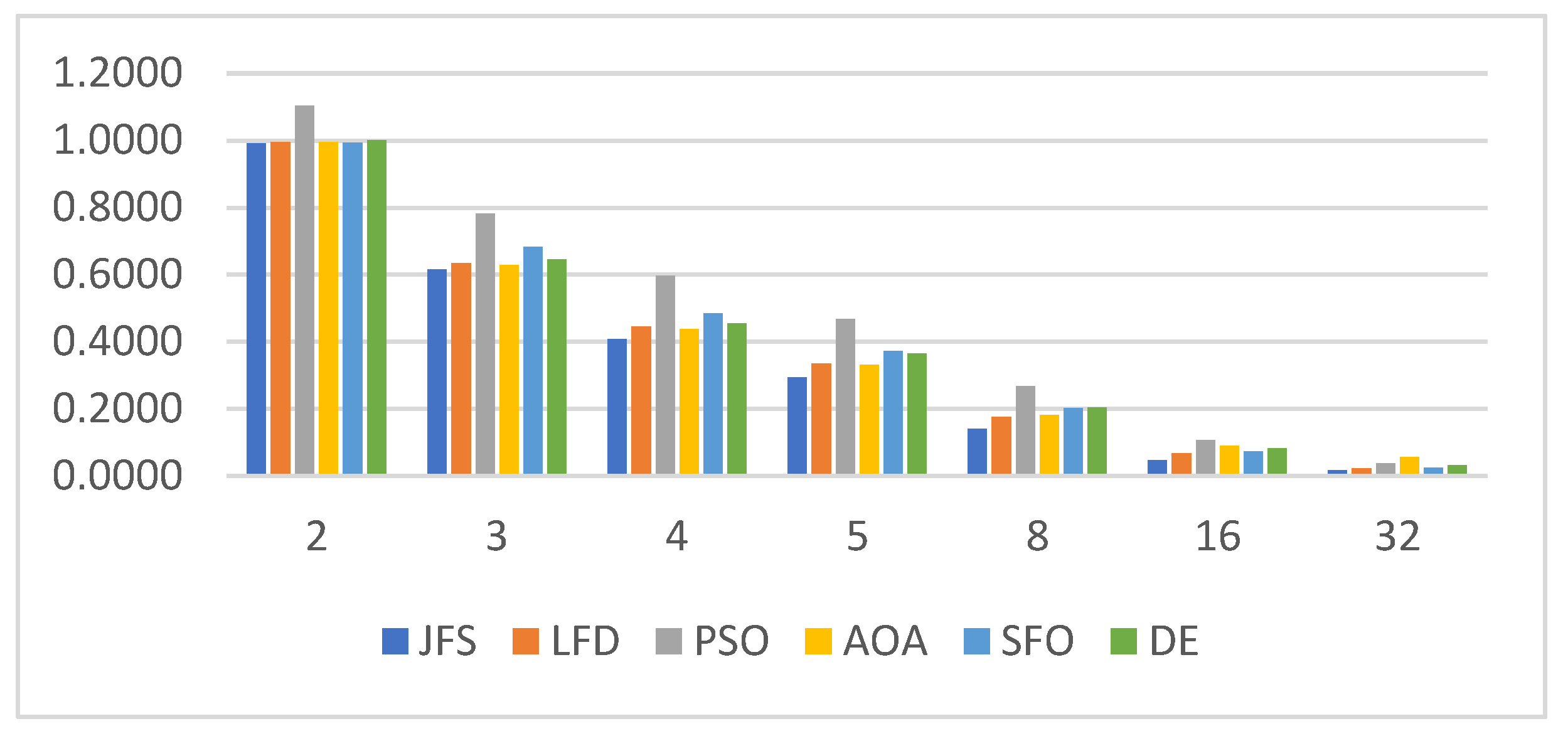
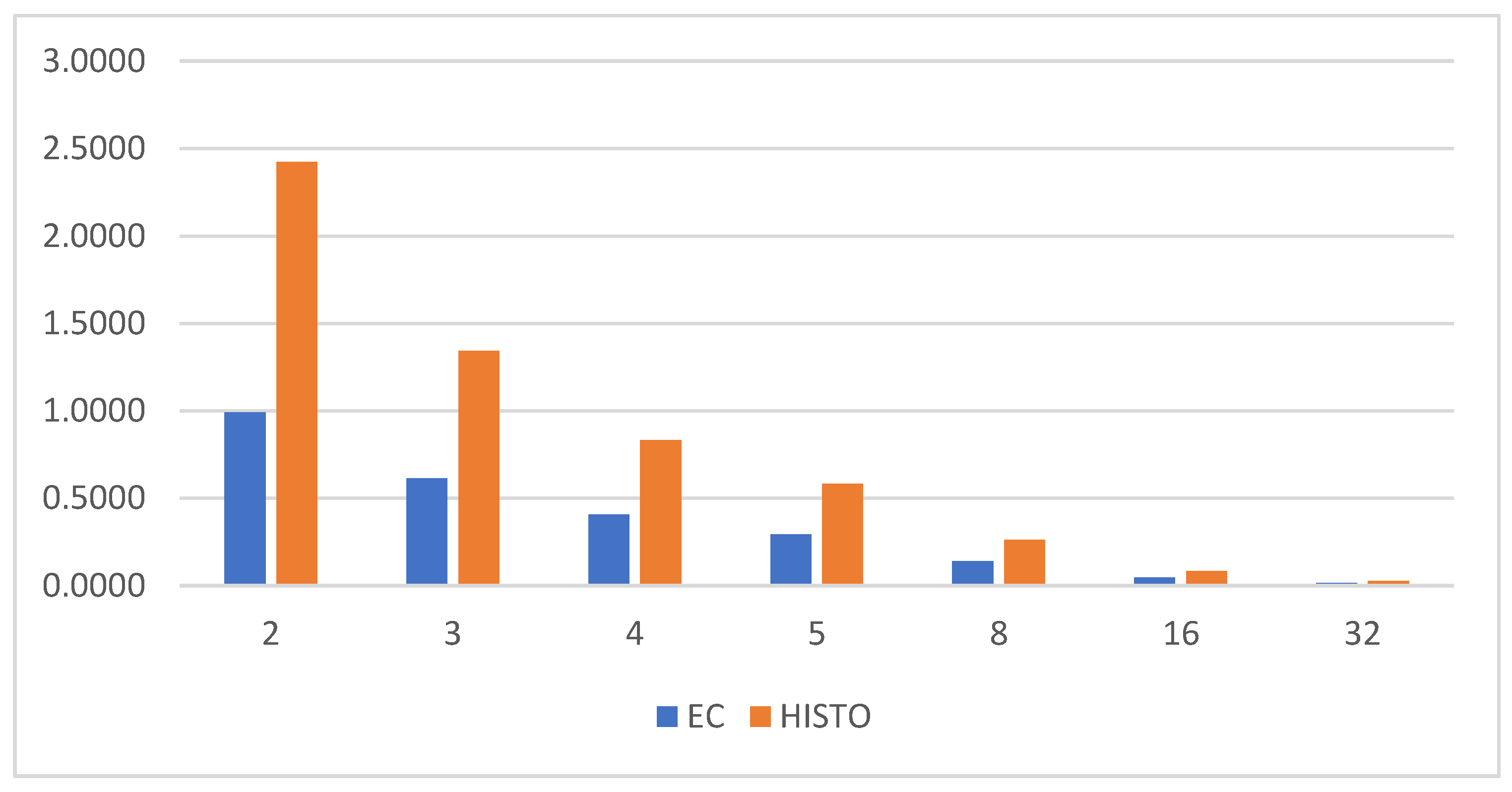
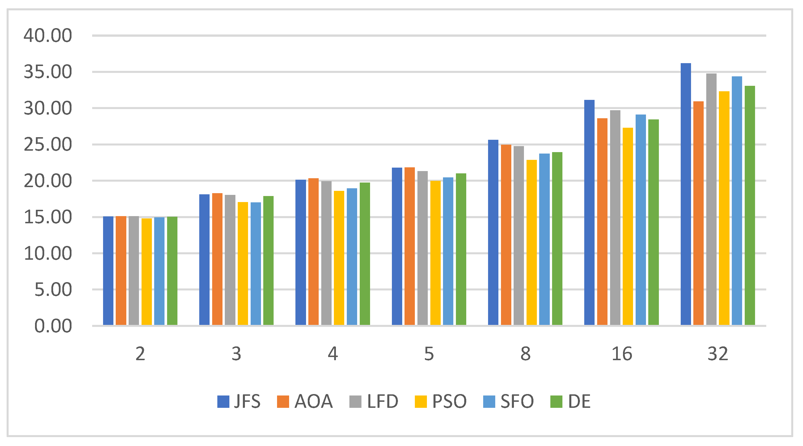
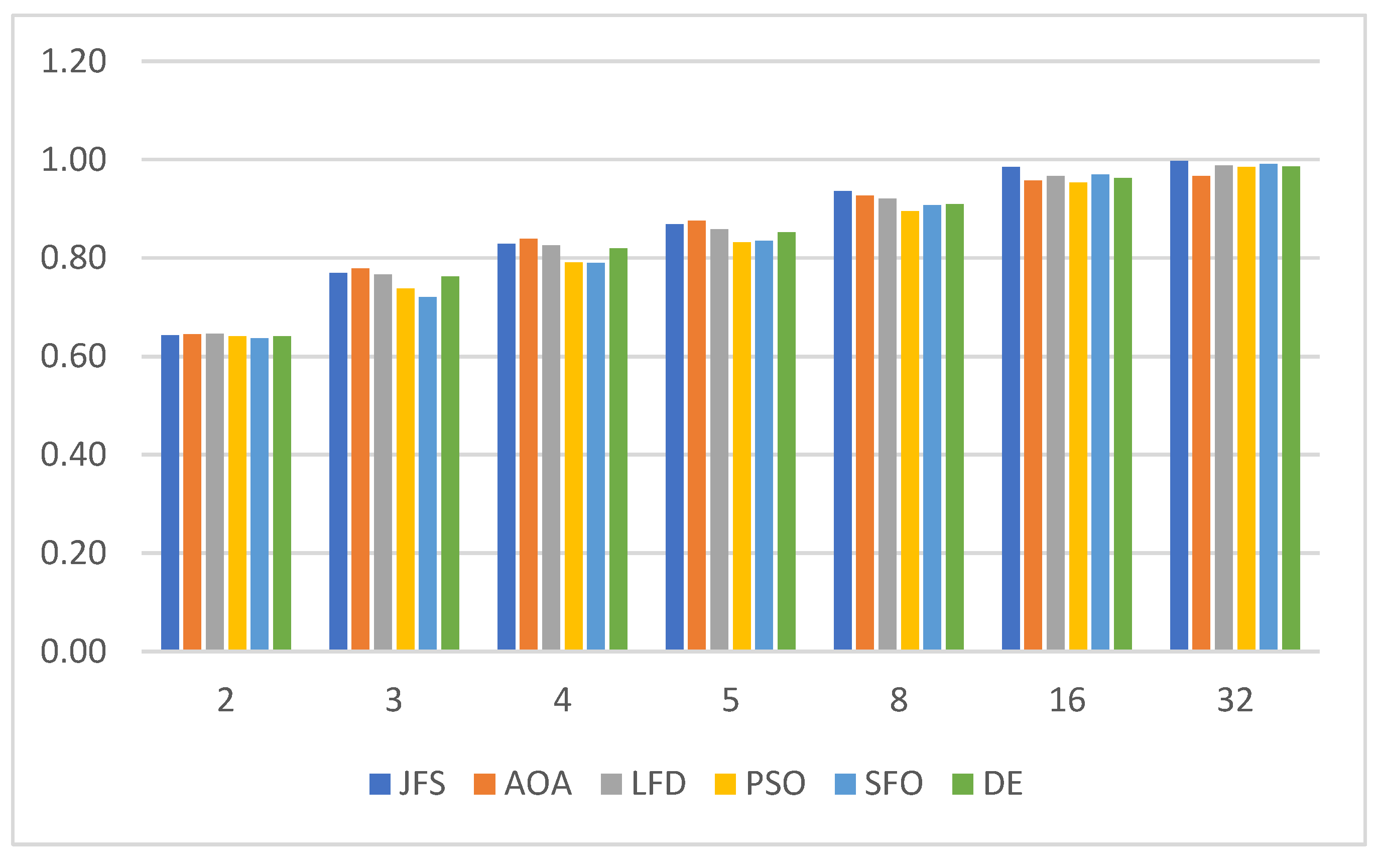
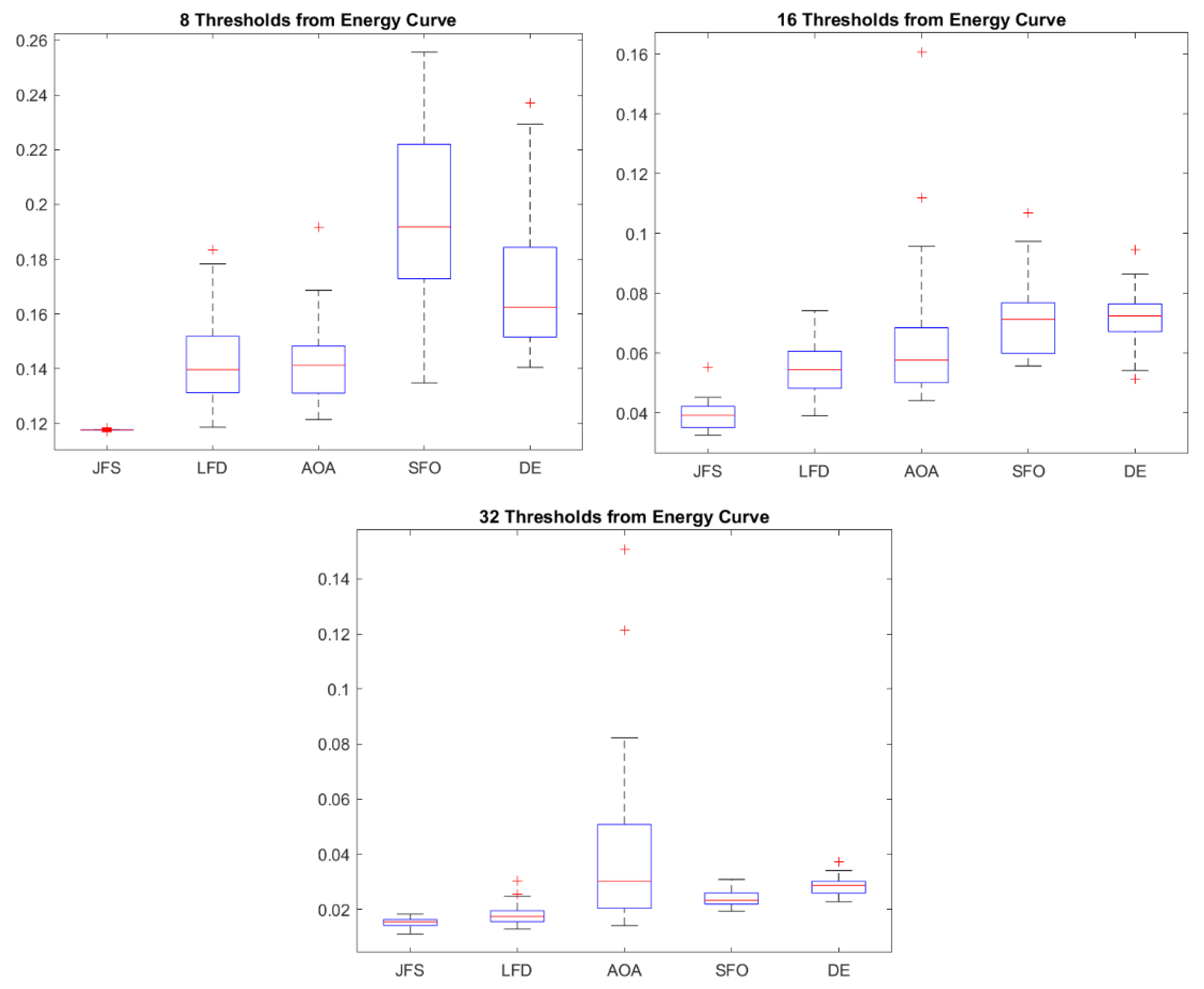
6.3. Statistical Analysis
7. Conclusions
Author Contributions
Funding
 , FODECYTJAL 2022, DISEÑO DE NUEVOS VEHÍCULOS SUSTENTABLES E INTELIGENTES EN JALISCO grant number 10300.
Data Availability Statement
Conflicts of Interest
References
- Gao, C.A.; Markov, N.S.; Stoeger, T.; Pawlowski, A.E.; Kang, M.; Nannapaneni, P.; Grant, R.A.; Pickens, C.; Walter, J.M.; Kruser, J.M.; et al. Machine learning links unresolving secondary pneumonia to mortality in patients with severe pneumonia, including COVID-19. J. Clin. Investig. 2023, 133, e170682. [Google Scholar] [CrossRef]
- Abdullah, S.H.; Abedi, W.M.S.; Hadi, R.M. Enhanced feature selection algorithm for pneumonia detection. Period. Eng. Nat. Sci. 2023, 10, 168–180. [Google Scholar] [CrossRef]
- Xie, P.; Zhao, X.; He, X. Improve the performance of CT-based pneumonia classification via source data reweighting. Sci. Rep. 2023, 13, 9401. [Google Scholar] [CrossRef] [PubMed]
- Yan, N.; Tao, Y. Pneumonia X-ray detection with anchor-free detection framework and data augmentation. Int. J. Imaging Syst. Technol. 2023, 33, 1235–1246. [Google Scholar] [CrossRef]
- Asswin, C.R.; KS, D.K.; Dora, A.; Ravi, V.; Sowmya, V.; Gopalakrishnan, E.A.; Soman, K.P. Transfer learning approach for pediatric pneumonia diagnosis using channel attention deep CNN architectures. Eng. Appl. Artif. Intell. 2023, 123, 106416. [Google Scholar]
- Kaya, Y.; Gürsoy, E. A MobileNet-based CNN model with a novel fine-tuning mechanism for COVID-19 infection detection. Soft Comput. 2023, 27, 5521–5535. [Google Scholar] [CrossRef] [PubMed]
- Chen, S.; Ren, S.; Wang, G.; Huang, M.; Xue, C. Interpretable CNN-Multilevel Attention Transformer for Rapid Recognition of Pneumonia from Chest X-ray Images. IEEE J. Biomed. Health Inform. 2023; online ahead of print. [Google Scholar]
- Sanghvi, H.A.; Patel, R.H.; Agarwal, A.; Gupta, S.; Sawhney, V.; Pandya, A.S. A deep learning approach for classification of COVID and pneumonia using DenseNet-201. Int. J. Imaging Syst. Technol. 2023, 33, 18–38. [Google Scholar] [CrossRef]
- AnbuDevi, M.K.A.; Suganthi, K. Review of Semantic Segmentation of Medical Images Using Modified Architectures of UNET. Diagnostics 2022, 12, 3064. [Google Scholar] [CrossRef]
- Zhou, Z.; Siddiquee, M.M.R.; Tajbakhsh, N.; Liang, J. Unet++: Redesigning skip connections to exploit multiscale features in image segmentation. IEEE Trans. Med. Imaging 2019, 39, 1856–1867. [Google Scholar] [CrossRef]
- Diakogiannis, F.I.; Waldner, F.; Caccetta, P.; Wu, C. ResUNet-a: A deep learning framework for semantic segmentation of remotely sensed data. ISPRS J. Photogramm. Remote Sens. 2020, 162, 94–114. [Google Scholar] [CrossRef]
- Li, X.; Chen, H.; Qi, X.; Dou, Q.; Fu, C.W.; Heng, P.A. H-DenseUNet: Hybrid densely connected UNet for liver and tumor segmentation from CT volumes. IEEE Trans. Med. Imaging 2018, 37, 2663–2674. [Google Scholar] [CrossRef] [PubMed]
- Aiadi, O.; Khaldi, B. A fast lightweight network for the discrimination of COVID-19 and pulmonary diseases. Biomed. Signal Process. Control 2022, 78, 103925. [Google Scholar] [CrossRef]
- Basu, A.; Sheikh, K.H.; Cuevas, E.; Sarkar, R. COVID-19 detection from CT scans using a two-stage framework. Expert Syst. Appl. 2022, 193, 116377. [Google Scholar] [CrossRef]
- Xue, X.; Chinnaperumal, S.; Abdulsahib, G.M.; Manyam, R.R.; Marappan, R.; Raju, S.K.; Khalaf, O.I. Design and Analysis of a Deep Learning Ensemble Framework Model for the Detection of COVID-19 and Pneumonia Using Large-Scale CT Scan and X-ray Image Datasets. Bioengineering 2023, 10, 363. [Google Scholar] [CrossRef] [PubMed]
- Issa, M.; Helmi, A.M.; Elsheikh, A.H.; Abd Elaziz, M. A biological sub-sequences detection using integrated BA-PSO based on infection propagation mechanism: Case study COVID-19. Expert Syst. Appl. 2022, 189, 116063. [Google Scholar] [CrossRef] [PubMed]
- Abualigah, L.; Diabat, A.; Sumari, P.; Gandomi, A.H. A novel evolutionary arithmetic optimization algorithm for multilevel thresholding segmentation of COVID-19 ct images. Processes 2021, 9, 1155. [Google Scholar] [CrossRef]
- Kumar, N.M.; Premalatha, K.; Suvitha, S. Lung disease detection using Self-Attention Generative Adversarial Capsule network optimized with sun flower Optimization Algorithm. Biomed. Signal Process. Control 2023, 79, 104241. [Google Scholar]
- Singh, D.; Kumar, V.; Vaishali; Kaur, M. Classification of COVID-19 patients from chest CT images using multi-objective differential evolution–based convolutional neural networks. Eur. J. Clin. Microbiol. Infect. Dis. 2020, 39, 1379–1389. [Google Scholar] [CrossRef]
- Chou, J.-S.; Ngo, N.-T. Modified firefly algorithm for multidimensional optimization in structural design problems. Struct. Multidiscip. Optim. 2017, 55, 2013–2028. [Google Scholar] [CrossRef]
- Shaheen, A.M.; El-Sehiemy, R.A.; Alharthi, M.M.; Ghoneim, S.S.; Ginidi, A.R. Multi-objective jellyfish search optimizer for efficient power system operation based on multi-dimensional OPF framework. Energy 2021, 237, 121478. [Google Scholar] [CrossRef]
- Kaveh, A.; Biabani Hamedani, K.; Kamalinejad, M.; Joudaki, A. Quantum-based jellyfish search optimizer for structural optimization. Int. J. Optim. Civil. Eng. 2021, 11, 329–356. [Google Scholar]
- Farhat, M.; Kamel, S.; Atallah, A.M.; Khan, B. Optimal power flow solution based on jellyfish search optimization considering uncertainty of renewable energy sources. IEEE Access 2021, 9, 100911–100933. [Google Scholar] [CrossRef]
- Oliva, D.; Hinojosa, S.; Osuna-Enciso, V.; Cuevas, E.; Pérez-Cisneros, M.; Sanchez-Ante, G. Image segmentation by minimum cross entropy using evolutionary methods. Soft Comput. 2019, 23, 431–450. [Google Scholar] [CrossRef]
- Kullback, S. Information Theory and Statistics; Courier Corporation: Chelmsford, MA, USA, 1997. [Google Scholar]
- Li, C.H.; Lee, C.K. Minimum cross entropy thresholding. Pattern Recognit. 1993, 26, 617–625. [Google Scholar] [CrossRef]
- Hammouche, K.; Diaf, M.; Siarry, P. A comparative study of various meta-heuristic techniques applied to the multilevel thresholding problem. Eng. Appl. Artif. Intell. 2010, 23, 676–688. [Google Scholar] [CrossRef]
- Sankur, B.; Sezgin, M. Survey over image thresholding techniques and quantitative performance evaluation. J. Electron. Imaging 2004, 13, 146–168. [Google Scholar] [CrossRef]
- Ghosh, S.; Bruzzone, L.; Patra, S.; Bovolo, F.; Ghosh, A. A contextsensitive technique for unsupervised change detection based on hopfield hopfieldtype neural networks. IEEE Trans. Geosci. Remote. Sens. 2007, 45, 778–789. [Google Scholar] [CrossRef]
- Patra, S.; Gautam, R.; Singla, A. A novel context sensitive multilevel thresholding for image segmentation. Appl. Soft Comput. 2014, 23, 122–127. [Google Scholar] [CrossRef]
- Oliva, D.; Hinojosa, S.; Abd Elaziz, M.; Ortega-Sánchez, N. Context based image segmentation using antlion optimization and sine cosine algorithm. Multimed. Tools Appl. 2018, 77, 25761–25797. [Google Scholar] [CrossRef]
- Houssein, E.H.; Saad, M.R.; Hashim, F.A.; Shaban, H.; Hassaballah, M. L′evy flight distribution: A new metaheuristic algorithm for solving engineering optimization problems. Eng. Appl. Artif. Intell. 2020, 94, 103731. [Google Scholar] [CrossRef]
- Kennedy, J.; Eberhart, R. Particle swarm optimization. In Proceedings of the ICNN’95-International Conference on Neural Networks, Perth, WA, Australia, 27 November–1 December 1995; IEEE: Piscataway, NJ, USA, 1995; Volume 4, pp. 1942–1948. [Google Scholar]
- Maitra, M.; Chatterjee, A. A hybrid cooperative–comprehensive learning based pso algorithm for image segmentation using multilevel thresholding. Expert Syst. Appl. 2008, 34, 1341–1350. [Google Scholar] [CrossRef]
- Xiang, T.; Liao, X.; Wong, K.-W. An improved particle swarm optimization algorithm combined with piecewise linear chaotic map. Appl. Math. Comput. 2007, 190, 1637–1645. [Google Scholar] [CrossRef]
- Abualigah, L.; Diabat, A.; Mirjalili, S.; Abd Elaziz, M.; Gandomi, A.H. The arithmetic optimization algorithm. Comput. Methods Appl. Mech. Eng. 2021, 376, 113609. [Google Scholar] [CrossRef]
- Khatir, S.; Tiachacht, S.; Le Thanh, C.; Ghandourah, E.; Mirjalili, S.; Wahab, M.A. An improved artificial neural network using arithmetic optimization algorithm for damage assessment in fgm composite plates. Compos. Struct. 2021, 273, 114287. [Google Scholar] [CrossRef]
- Gomes, G.F.; da Cunha, S.S., Jr.; Ancelotti, A.C. A sunflower optimization (sfo) algorithm applied to damage identification on laminated composite plates. Eng. Comput. 2019, 35, 619–626. [Google Scholar] [CrossRef]
- Yuan, Z.; Wang, W.; Wang, H.; Razmjooy, N. A new technique for optimal estimation of the circuit-based pemfcs using developed sunflower optimization algorithm. Energy Rep. 2020, 6, 662–671. [Google Scholar] [CrossRef]
- Chou, J.-S.; Truong, D.-N. A novel metaheuristic optimizer inspired by behavior of jellyfish in ocean. Appl. Math. Comput. 2021, 389, 125535. [Google Scholar] [CrossRef]
- Fossette, S.; Gleiss, A.C.; Chalumeau, J.; Bastian, T.; Armstrong, C.D.; Vandenabeele, S.; Karpytchev, M.; Hays, G.C. Current-oriented swimming by jellyfish and its role in bloom maintenance. Curr. Biol. 2015, 25, 342–347. [Google Scholar] [CrossRef]
- Storn, R.; Price, K. Differential evolution—A simple and efficient heuristic for global optimization over continuous spaces. J. Glob. Optim. 1997, 11, 341–359. [Google Scholar] [CrossRef]
- Cuevas, E.; Zaldivar, D.; Pérez-Cisneros, M. A novel multi-threshold segmentation approach based on differential evolution optimization. Expert Syst. Appl. 2010, 37, 5265–5271. [Google Scholar] [CrossRef]
- Avcibas, I.; Sankur, B.; Sayood, K. Statistical evaluation of image quality measures. J. Electron. Imaging 2002, 11, 206–223. [Google Scholar]
- Wang, Z.; Bovik, A.C.; Sheikh, H.R.; Simoncelli, E.P. Image quality assessment: From error visibility to structural similarity. IEEE Trans. Image Process. 2004, 13, 600–612. [Google Scholar] [CrossRef]
- Zhang, L.; Zhang, L.; Mou, X.; Zhang, D. FSIM: A feature similarity index for image quality assessment. IEEE Trans. Image Process. 2011, 20, 2378–2386. [Google Scholar] [CrossRef] [PubMed]
- Kaggle. Chest X-ray Images (Pneumonia). 10 February 2018. Available online: https://www.kaggle.com/datasets/paultimothymooney/chest-xray-pneumonia (accessed on 24 August 2023).
- Theodorsson-Norheim, E. Kruskal-wallis test: Basic computer program to perform nonparametric one-way analysis of variance and multiple comparisons on ranks of several independent samples. Comput. Methods Programs Biomed. 1986, 23, 57–62. [Google Scholar] [CrossRef] [PubMed]
- Scheffe, H. The Analysis of Variance; John Wiley & Sons: Hoboken, NJ, USA, 1999; Volume 72. [Google Scholar]


| Algorithm | Parameters | Value |
|---|---|---|
| Levy flight distribution (LFD) | Search agents no | 30 |
| Max iterations | 1000 | |
| Particle swarm optimization (PSO) | Social coefficient | 2 |
| Cognitive coefficient | 2 | |
| Velocity clamp | 2 | |
| Maximum inertia value | 0.2 | |
| Minimum inertia value | 0.9 | |
| Arithmetic optimization algorithm (AOA) | Materials number | 30 |
| Max iterations | 1000 | |
| Optimization functions | 2, 6 | |
| Sunflower optimization (SFO) | Number of sunflowers | 60 |
| Number of experiments | 30 | |
| Pollination values | 0.05 | |
| Mortality rate, best values | 0.1 | |
| Survival rate | 1-(p + m) | |
| Iterations/generations | 1000 | |
| Jellyfish search optimizer (JSO) | Number of decisions | 30 |
| Maximum number of iterations | 1000 | |
| Population size | 30 | |
| Differential evolution (DE) | Crossover rate | 0.5 |
| Number of experiments | 30 | |
| Scale factor | 0.2 |
| Image | LFD | PSO | AOA | SFO | JSO | DE | |||||||
|---|---|---|---|---|---|---|---|---|---|---|---|---|---|
| nt | Mean | Std | Mean | Std | Mean | Std | Mean | Std | Mean | Std | Mean | Std | |
| 2 | 0.745 | 0.005 | 0.854 | 0.072 | 0.744 | 0.004 | 0.744 | 0.001 | 0.743 | 0.000 | 0.752 | 0.017 | |
| 3 | 0.462 | 0.027 | 0.687 | 0.112 | 0.457 | 0.015 | 0.542 | 0.074 | 0.445 | 0.000 | 0.486 | 0.044 | |
| Image 01 | 4 | 0.329 | 0.018 | 0.471 | 0.076 | 0.324 | 0.012 | 0.418 | 0.074 | 0.309 | 0.000 | 0.357 | 0.044 |
| 5 | 0.251 | 0.019 | 0.401 | 0.086 | 0.247 | 0.019 | 0.334 | 0.046 | 0.226 | 0.000 | 0.302 | 0.040 | |
| 8 | 0.142 | 0.016 | 0.243 | 0.034 | 0.142 | 0.015 | 0.192 | 0.029 | 0.118 | 0.000 | 0.171 | 0.024 | |
| 16 | 0.055 | 0.010 | 0.092 | 0.017 | 0.065 | 0.024 | 0.072 | 0.012 | 0.039 | 0.005 | 0.072 | 0.009 | |
| 32 | 0.018 | 0.004 | 0.035 | 0.006 | 0.042 | 0.032 | 0.024 | 0.003 | 0.015 | 0.002 | 0.029 | 0.004 | |
| nt | Mean | Std | Mean | Std | Mean | Std | Mean | Std | Mean | Std | Mean | Std | |
| 2 | 0.926 | 0.004 | 0.985 | 0.025 | 0.926 | 0.006 | 0.926 | 0.002 | 0.924 | 0.000 | 0.930 | 0.009 | |
| 3 | 0.593 | 0.018 | 0.728 | 0.105 | 0.589 | 0.019 | 0.658 | 0.078 | 0.576 | 0.000 | 0.607 | 0.038 | |
| Image 02 | 4 | 0.421 | 0.028 | 0.567 | 0.086 | 0.409 | 0.013 | 0.488 | 0.070 | 0.394 | 0.000 | 0.428 | 0.024 |
| 5 | 0.312 | 0.023 | 0.475 | 0.092 | 0.315 | 0.043 | 0.375 | 0.064 | 0.277 | 0.000 | 0.337 | 0.033 | |
| 8 | 0.169 | 0.015 | 0.259 | 0.034 | 0.181 | 0.054 | 0.209 | 0.031 | 0.135 | 0.000 | 0.199 | 0.028 | |
| 16 | 0.065 | 0.011 | 0.103 | 0.016 | 0.082 | 0.036 | 0.072 | 0.012 | 0.050 | 0.004 | 0.080 | 0.011 | |
| 32 | 0.023 | 0.003 | 0.038 | 0.005 | 0.043 | 0.021 | 0.024 | 0.004 | 0.018 | 0.003 | 0.032 | 0.004 | |
| nt | Mean | Std | Mean | Std | Mean | Std | Mean | Std | Mean | Std | Mean | Std | |
| 2 | 1.508 | 0.016 | 1.653 | 0.099 | 1.516 | 0.028 | 1.506 | 0.003 | 1.504 | 0.000 | 1.519 | 0.020 | |
| 3 | 0.962 | 0.024 | 0.996 | 0.012 | 0.960 | 0.028 | 0.985 | 0.044 | 0.932 | 0.000 | 0.963 | 0.032 | |
| Image 03 | 4 | 0.653 | 0.065 | 0.796 | 0.112 | 0.651 | 0.060 | 0.638 | 0.046 | 0.574 | 0.000 | 0.630 | 0.056 |
| 5 | 0.469 | 0.048 | 0.614 | 0.089 | 0.465 | 0.045 | 0.469 | 0.062 | 0.395 | 0.000 | 0.482 | 0.035 | |
| 8 | 0.232 | 0.034 | 0.327 | 0.028 | 0.237 | 0.059 | 0.242 | 0.039 | 0.176 | 0.000 | 0.256 | 0.026 | |
| 16 | 0.086 | 0.013 | 0.130 | 0.023 | 0.121 | 0.049 | 0.090 | 0.015 | 0.060 | 0.005 | 0.103 | 0.010 | |
| 32 | 0.032 | 0.005 | 0.043 | 0.007 | 0.096 | 0.060 | 0.028 | 0.006 | 0.021 | 0.002 | 0.038 | 0.004 | |
| nt | Mean | Std | Mean | Std | Mean | Std | Mean | Std | Mean | Std | Mean | Std | |
| 2 | 1.129 | 0.007 | 1.294 | 0.159 | 1.127 | 0.006 | 1.127 | 0.001 | 1.125 | 0.000 | 1.135 | 0.014 | |
| 3 | 0.717 | 0.026 | 0.882 | 0.090 | 0.718 | 0.020 | 0.788 | 0.106 | 0.700 | 0.000 | 0.741 | 0.050 | |
| Image 04 | 4 | 0.502 | 0.038 | 0.707 | 0.089 | 0.492 | 0.021 | 0.558 | 0.075 | 0.465 | 0.000 | 0.520 | 0.038 |
| 5 | 0.395 | 0.037 | 0.536 | 0.077 | 0.371 | 0.028 | 0.428 | 0.058 | 0.335 | 0.000 | 0.419 | 0.047 | |
| 8 | 0.208 | 0.028 | 0.312 | 0.055 | 0.209 | 0.053 | 0.238 | 0.031 | 0.162 | 0.000 | 0.233 | 0.027 | |
| 16 | 0.078 | 0.010 | 0.122 | 0.014 | 0.104 | 0.043 | 0.085 | 0.014 | 0.056 | 0.005 | 0.096 | 0.012 | |
| 32 | 0.027 | 0.004 | 0.040 | 0.005 | 0.057 | 0.042 | 0.027 | 0.004 | 0.019 | 0.002 | 0.035 | 0.004 | |
| nt | Mean | Std | Mean | Std | Mean | Std | Mean | Std | Mean | Std | Mean | Std | |
| 2 | 1.007 | 0.005 | 1.141 | 0.115 | 1.009 | 0.025 | 1.007 | 0.002 | 1.004 | 0.000 | 1.016 | 0.028 | |
| 3 | 0.673 | 0.020 | 0.792 | 0.093 | 0.666 | 0.014 | 0.711 | 0.056 | 0.655 | 0.000 | 0.685 | 0.028 | |
| Image 05 | 4 | 0.470 | 0.034 | 0.614 | 0.080 | 0.464 | 0.025 | 0.500 | 0.070 | 0.432 | 0.000 | 0.467 | 0.029 |
| 5 | 0.362 | 0.029 | 0.491 | 0.071 | 0.355 | 0.023 | 0.396 | 0.047 | 0.325 | 0.000 | 0.387 | 0.035 | |
| 8 | 0.189 | 0.019 | 0.279 | 0.037 | 0.203 | 0.047 | 0.211 | 0.030 | 0.155 | 0.000 | 0.226 | 0.029 | |
| 16 | 0.073 | 0.012 | 0.111 | 0.015 | 0.097 | 0.034 | 0.070 | 0.009 | 0.048 | 0.004 | 0.087 | 0.009 | |
| 32 | 0.025 | 0.005 | 0.039 | 0.006 | 0.071 | 0.032 | 0.024 | 0.003 | 0.017 | 0.002 | 0.033 | 0.004 | |
| nt | Mean | Std | Mean | Std | Mean | Std | Mean | Std | Mean | Std | Mean | Std | |
| 2 | 0.767 | 0.005 | 0.840 | 0.057 | 0.765 | 0.001 | 0.765 | 0.001 | 0.764 | 0.000 | 0.768 | 0.005 | |
| 3 | 0.448 | 0.029 | 0.595 | 0.107 | 0.436 | 0.017 | 0.481 | 0.054 | 0.422 | 0.000 | 0.445 | 0.026 | |
| Image 06 | 4 | 0.316 | 0.024 | 0.452 | 0.065 | 0.303 | 0.015 | 0.358 | 0.053 | 0.285 | 0.000 | 0.329 | 0.035 |
| 5 | 0.237 | 0.027 | 0.333 | 0.055 | 0.242 | 0.031 | 0.280 | 0.035 | 0.205 | 0.000 | 0.266 | 0.036 | |
| 8 | 0.132 | 0.012 | 0.194 | 0.038 | 0.156 | 0.050 | 0.149 | 0.025 | 0.106 | 0.003 | 0.150 | 0.017 | |
| 16 | 0.050 | 0.008 | 0.078 | 0.013 | 0.067 | 0.017 | 0.055 | 0.008 | 0.034 | 0.003 | 0.062 | 0.011 | |
| 32 | 0.017 | 0.003 | 0.030 | 0.004 | 0.039 | 0.015 | 0.019 | 0.003 | 0.014 | 0.002 | 0.023 | 0.002 | |
| nt | Mean | Std | Mean | Std | Mean | Std | Mean | Std | Mean | Std | Mean | Std | |
| 2 | 0.839 | 0.008 | 0.933 | 0.064 | 0.835 | 0.002 | 0.836 | 0.002 | 0.834 | 0.000 | 0.842 | 0.013 | |
| 3 | 0.554 | 0.017 | 0.703 | 0.087 | 0.548 | 0.010 | 0.599 | 0.056 | 0.541 | 0.000 | 0.569 | 0.032 | |
| Image 07 | 4 | 0.412 | 0.022 | 0.545 | 0.054 | 0.398 | 0.014 | 0.430 | 0.033 | 0.382 | 0.000 | 0.430 | 0.030 |
| 5 | 0.313 | 0.020 | 0.436 | 0.054 | 0.307 | 0.025 | 0.329 | 0.033 | 0.281 | 0.000 | 0.339 | 0.035 | |
| 8 | 0.161 | 0.018 | 0.238 | 0.033 | 0.162 | 0.031 | 0.176 | 0.027 | 0.130 | 0.001 | 0.189 | 0.025 | |
| 16 | 0.058 | 0.008 | 0.096 | 0.013 | 0.081 | 0.034 | 0.062 | 0.010 | 0.042 | 0.002 | 0.075 | 0.008 | |
| 32 | 0.021 | 0.004 | 0.033 | 0.004 | 0.044 | 0.022 | 0.023 | 0.004 | 0.014 | 0.001 | 0.027 | 0.003 | |
| nt | Mean | Std | Mean | Std | Mean | Std | Mean | Std | Mean | Std | Mean | Std | |
| 2 | 1.039 | 0.004 | 1.187 | 0.144 | 1.036 | 0.000 | 1.038 | 0.003 | 1.036 | 0.000 | 1.046 | 0.021 | |
| 3 | 0.666 | 0.024 | 0.819 | 0.099 | 0.652 | 0.011 | 0.695 | 0.056 | 0.643 | 0.000 | 0.665 | 0.021 | |
| Image 08 | 4 | 0.451 | 0.023 | 0.634 | 0.091 | 0.449 | 0.020 | 0.482 | 0.051 | 0.421 | 0.000 | 0.477 | 0.049 |
| 5 | 0.339 | 0.040 | 0.490 | 0.064 | 0.320 | 0.030 | 0.358 | 0.045 | 0.292 | 0.000 | 0.381 | 0.059 | |
| 8 | 0.171 | 0.026 | 0.285 | 0.042 | 0.171 | 0.031 | 0.184 | 0.023 | 0.137 | 0.004 | 0.207 | 0.028 | |
| 16 | 0.064 | 0.010 | 0.112 | 0.019 | 0.073 | 0.019 | 0.075 | 0.011 | 0.047 | 0.003 | 0.083 | 0.011 | |
| 32 | 0.022 | 0.004 | 0.039 | 0.006 | 0.054 | 0.039 | 0.026 | 0.005 | 0.016 | 0.001 | 0.032 | 0.004 | |
| nt | Mean | Std | Mean | Std | Mean | Std | Mean | Std | Mean | Std | Mean | Std | |
| 2 | 1.028 | 0.004 | 1.153 | 0.121 | 1.029 | 0.007 | 1.028 | 0.002 | 1.026 | 0.000 | 1.033 | 0.011 | |
| 3 | 0.666 | 0.020 | 0.830 | 0.092 | 0.659 | 0.017 | 0.719 | 0.075 | 0.646 | 0.000 | 0.673 | 0.036 | |
| Image 09 | 4 | 0.476 | 0.032 | 0.615 | 0.091 | 0.463 | 0.022 | 0.509 | 0.076 | 0.430 | 0.000 | 0.469 | 0.026 |
| 5 | 0.344 | 0.024 | 0.470 | 0.064 | 0.360 | 0.039 | 0.394 | 0.067 | 0.307 | 0.000 | 0.372 | 0.039 | |
| 8 | 0.183 | 0.021 | 0.275 | 0.034 | 0.186 | 0.029 | 0.209 | 0.033 | 0.148 | 0.000 | 0.213 | 0.024 | |
| 16 | 0.073 | 0.013 | 0.110 | 0.016 | 0.114 | 0.064 | 0.072 | 0.010 | 0.051 | 0.003 | 0.086 | 0.011 | |
| 32 | 0.025 | 0.005 | 0.038 | 0.005 | 0.058 | 0.027 | 0.023 | 0.003 | 0.018 | 0.002 | 0.034 | 0.003 | |
| nt | Mean | Std | Mean | Std | Mean | Std | Mean | Std | Mean | Std | Mean | Std | |
| 2 | 0.964 | 0.003 | 0.996 | 0.010 | 0.962 | 0.000 | 0.963 | 0.001 | 0.962 | 0.000 | 0.968 | 0.009 | |
| 3 | 0.603 | 0.016 | 0.795 | 0.103 | 0.598 | 0.010 | 0.651 | 0.057 | 0.588 | 0.000 | 0.617 | 0.026 | |
| Image 10 | 4 | 0.418 | 0.026 | 0.564 | 0.117 | 0.419 | 0.015 | 0.467 | 0.049 | 0.395 | 0.000 | 0.439 | 0.041 |
| 5 | 0.322 | 0.024 | 0.437 | 0.045 | 0.322 | 0.020 | 0.350 | 0.031 | 0.293 | 0.000 | 0.356 | 0.037 | |
| 8 | 0.177 | 0.015 | 0.264 | 0.041 | 0.172 | 0.028 | 0.203 | 0.038 | 0.138 | 0.000 | 0.199 | 0.023 | |
| 16 | 0.066 | 0.013 | 0.107 | 0.021 | 0.094 | 0.045 | 0.067 | 0.009 | 0.046 | 0.004 | 0.079 | 0.009 | |
| 32 | 0.021 | 0.004 | 0.036 | 0.005 | 0.048 | 0.037 | 0.024 | 0.004 | 0.016 | 0.002 | 0.030 | 0.003 | |
| Image | LFD | PSO | AOA | SFO | JSO | DE | |||||||
|---|---|---|---|---|---|---|---|---|---|---|---|---|---|
| nt | Mean | Std | Mean | Std | Mean | Std | Mean | Std | Mean | Std | Mean | Std | |
| 2 | 1.1776 | 0.0064 | 1.3242 | 0.1246 | 1.1759 | 0.0033 | 1.1766 | 0.0018 | 1.1748 | 0.0000 | 1.1887 | 0.0246 | |
| 3 | 0.8071 | 0.0266 | 0.8920 | 0.0615 | 0.8176 | 0.0228 | 0.8236 | 0.0443 | 0.7741 | 0.0000 | 0.8036 | 0.0332 | |
| Image 01 | 4 | 0.5395 | 0.0657 | 0.6869 | 0.0913 | 0.5298 | 0.0396 | 0.5262 | 0.0628 | 0.4704 | 0.0000 | 0.5163 | 0.0395 |
| 5 | 0.3713 | 0.0540 | 0.5286 | 0.0770 | 0.3731 | 0.0511 | 0.3758 | 0.0481 | 0.3183 | 0.0000 | 0.4015 | 0.0541 | |
| 8 | 0.1894 | 0.0324 | 0.2956 | 0.0439 | 0.1993 | 0.0338 | 0.2141 | 0.0458 | 0.1441 | 0.0002 | 0.2144 | 0.0317 | |
| 16 | 0.0690 | 0.0093 | 0.1186 | 0.0163 | 0.1111 | 0.0824 | 0.0787 | 0.0131 | 0.0527 | 0.0045 | 0.0948 | 0.0116 | |
| 32 | 0.0283 | 0.0045 | 0.0404 | 0.0050 | 0.0695 | 0.0357 | 0.0264 | 0.0040 | 0.0200 | 0.0019 | 0.0351 | 0.0045 | |
| nt | Mean | Std | Mean | Std | Mean | Std | Mean | Std | Mean | Std | Mean | Std | |
| 2 | 2.3187 | 0.0417 | 2.5176 | 0.2269 | 2.3022 | 0.0387 | 2.2925 | 0.0032 | 2.2896 | 0.0000 | 2.3127 | 0.0428 | |
| 3 | 1.2947 | 0.0794 | 1.5137 | 0.1800 | 1.3436 | 0.1210 | 1.3396 | 0.0889 | 1.2642 | 0.0000 | 1.3318 | 0.0932 | |
| Image 02 | 4 | 0.8603 | 0.0801 | 0.9726 | 0.0510 | 0.9114 | 0.1640 | 0.8097 | 0.0417 | 0.7645 | 0.0001 | 0.8431 | 0.0525 |
| 5 | 0.6201 | 0.0890 | 0.8095 | 0.1272 | 0.6301 | 0.1201 | 0.5829 | 0.0601 | 0.5110 | 0.0000 | 0.6096 | 0.0681 | |
| 8 | 0.3142 | 0.0516 | 0.4328 | 0.0714 | 0.3624 | 0.1678 | 0.2821 | 0.0385 | 0.2314 | 0.0002 | 0.3676 | 0.0459 | |
| 16 | 0.1076 | 0.0182 | 0.1687 | 0.0278 | 0.1750 | 0.0601 | 0.0997 | 0.0121 | 0.0785 | 0.0045 | 0.1366 | 0.0197 | |
| 32 | 0.0370 | 0.0053 | 0.0593 | 0.0077 | 0.1239 | 0.0545 | 0.0331 | 0.0058 | 0.0251 | 0.0023 | 0.0497 | 0.0063 | |
| nt | Mean | Std | Mean | Std | Mean | Std | Mean | Std | Mean | Std | Mean | Std | |
| 2 | 2.4743 | 0.0579 | 2.6656 | 0.2290 | 2.4645 | 0.0472 | 2.4494 | 0.0038 | 2.4457 | 0.0000 | 2.4564 | 0.0244 | |
| 3 | 1.3733 | 0.0635 | 1.7253 | 0.2550 | 1.4008 | 0.1516 | 1.3780 | 0.0495 | 1.3219 | 0.0000 | 1.3950 | 0.0830 | |
| Image 03 | 4 | 0.9710 | 0.0651 | 0.9953 | 0.0169 | 0.9723 | 0.1114 | 0.9545 | 0.0452 | 0.8893 | 0.0000 | 0.9889 | 0.0697 |
| 5 | 0.7469 | 0.0637 | 0.9300 | 0.0915 | 0.7401 | 0.1024 | 0.7204 | 0.0420 | 0.6595 | 0.0001 | 0.7568 | 0.0645 | |
| 8 | 0.4304 | 0.0422 | 0.5392 | 0.0722 | 0.4940 | 0.1470 | 0.3816 | 0.0474 | 0.3107 | 0.0007 | 0.4630 | 0.0361 | |
| 16 | 0.1633 | 0.0231 | 0.2189 | 0.0302 | 0.3118 | 0.1492 | 0.1420 | 0.0207 | 0.0999 | 0.0043 | 0.1817 | 0.0237 | |
| 32 | 0.0555 | 0.0081 | 0.0841 | 0.0105 | 0.2387 | 0.1231 | 0.0486 | 0.0086 | 0.0323 | 0.0022 | 0.0705 | 0.0091 | |
| nt | Mean | Std | Mean | Std | Mean | Std | Mean | Std | Mean | Std | Mean | Std | |
| 2 | 2.9575 | 0.0265 | 3.1800 | 0.1497 | 2.9484 | 0.0177 | 2.9448 | 0.0031 | 2.9424 | 0.0000 | 2.9695 | 0.0484 | |
| 3 | 1.6539 | 0.1259 | 1.8682 | 0.2265 | 1.6062 | 0.0484 | 1.6274 | 0.0790 | 1.5613 | 0.0001 | 1.6252 | 0.0827 | |
| Image 04 | 4 | 1.0546 | 0.0718 | 1.0976 | 0.2086 | 1.1092 | 0.1502 | 1.0562 | 0.0672 | 0.9777 | 0.0000 | 1.1278 | 0.1465 |
| 5 | 0.7976 | 0.0831 | 0.9739 | 0.0546 | 0.8455 | 0.1374 | 0.7401 | 0.0548 | 0.6769 | 0.0001 | 0.7977 | 0.0947 | |
| 8 | 0.3875 | 0.0555 | 0.5586 | 0.0961 | 0.4342 | 0.1049 | 0.3553 | 0.0493 | 0.2886 | 0.0004 | 0.4239 | 0.0519 | |
| 16 | 0.1316 | 0.0242 | 0.2116 | 0.0321 | 0.2572 | 0.1239 | 0.1125 | 0.0106 | 0.0845 | 0.0033 | 0.1607 | 0.0183 | |
| 32 | 0.0430 | 0.0066 | 0.0665 | 0.0088 | 0.1977 | 0.1859 | 0.0366 | 0.0062 | 0.0268 | 0.0016 | 0.0573 | 0.0074 | |
| nt | Mean | Std | Mean | Std | Mean | Std | Mean | Std | Mean | Std | Mean | Std | |
| 2 | 2.6902 | 0.0433 | 2.9984 | 0.4064 | 2.6679 | 0.0037 | 2.6676 | 0.0031 | 2.6652 | 0.0000 | 2.6840 | 0.0382 | |
| 3 | 1.5643 | 0.0891 | 1.9372 | 0.2832 | 1.5931 | 0.1841 | 1.5654 | 0.0830 | 1.4956 | 0.0000 | 1.5672 | 0.0839 | |
| Image 05 | 4 | 1.0150 | 0.0890 | 1.0000 | 0.0000 | 1.0314 | 0.1375 | 0.9610 | 0.0637 | 0.8911 | 0.0000 | 1.0470 | 0.1239 |
| 5 | 0.7420 | 0.0495 | 0.9475 | 0.0771 | 0.7330 | 0.1328 | 0.7226 | 0.0730 | 0.6633 | 0.0004 | 0.8292 | 0.0900 | |
| 8 | 0.4242 | 0.0554 | 0.5849 | 0.0931 | 0.4735 | 0.2178 | 0.3879 | 0.0507 | 0.2961 | 0.0018 | 0.4588 | 0.0525 | |
| 16 | 0.1489 | 0.0343 | 0.2428 | 0.0402 | 0.2525 | 0.0501 | 0.1280 | 0.0252 | 0.0932 | 0.0055 | 0.1824 | 0.0292 | |
| 32 | 0.0514 | 0.0091 | 0.0802 | 0.0096 | 0.1680 | 0.0898 | 0.0428 | 0.0079 | 0.0307 | 0.0020 | 0.0665 | 0.0083 | |
| nt | Mean | Std | Mean | Std | Mean | Std | Mean | Std | Mean | Std | Mean | Std | |
| 2 | 2.3123 | 0.0279 | 2.5947 | 0.2414 | 2.2991 | 0.0041 | 2.3001 | 0.0037 | 2.2968 | 0.0000 | 2.3144 | 0.0275 | |
| 3 | 1.2900 | 0.0972 | 1.7208 | 0.2684 | 1.2855 | 0.0642 | 1.3007 | 0.1017 | 1.2079 | 0.0001 | 1.2994 | 0.0759 | |
| Image 06 | 4 | 0.8801 | 0.1110 | 0.9972 | 0.0152 | 0.8824 | 0.1116 | 0.8218 | 0.0779 | 0.7305 | 0.0000 | 0.8545 | 0.1110 |
| 5 | 0.6220 | 0.1001 | 0.8507 | 0.1469 | 0.6455 | 0.1103 | 0.6107 | 0.0940 | 0.5029 | 0.0000 | 0.6501 | 0.1031 | |
| 8 | 0.3101 | 0.0477 | 0.4769 | 0.0964 | 0.3402 | 0.0855 | 0.2965 | 0.0459 | 0.2172 | 0.0078 | 0.3439 | 0.0674 | |
| 16 | 0.1106 | 0.0200 | 0.1872 | 0.0358 | 0.1979 | 0.1120 | 0.1058 | 0.0155 | 0.0686 | 0.0037 | 0.1460 | 0.0185 | |
| 32 | 0.0363 | 0.0072 | 0.0655 | 0.0110 | 0.1284 | 0.0593 | 0.0361 | 0.0053 | 0.0223 | 0.0016 | 0.0513 | 0.0069 | |
| nt | Mean | Std | Mean | Std | Mean | Std | Mean | Std | Mean | Std | Mean | Std | |
| 2 | 2.9113 | 0.0252 | 3.3521 | 0.3679 | 2.9029 | 0.0029 | 2.9067 | 0.0085 | 2.9015 | 0.0000 | 2.9546 | 0.0767 | |
| 3 | 1.5846 | 0.0734 | 2.1718 | 0.4024 | 1.6081 | 0.0860 | 1.6325 | 0.0894 | 1.5407 | 0.0001 | 1.6051 | 0.0685 | |
| Image 07 | 4 | 1.0540 | 0.0973 | 1.3216 | 0.4585 | 1.0361 | 0.0753 | 1.1058 | 0.1222 | 0.9607 | 0.0001 | 1.1419 | 0.1740 |
| 5 | 0.7592 | 0.0917 | 0.9908 | 0.0253 | 0.7746 | 0.0775 | 0.7749 | 0.0817 | 0.6492 | 0.0001 | 0.8810 | 0.1170 | |
| 8 | 0.3907 | 0.0544 | 0.6640 | 0.1495 | 0.4343 | 0.1039 | 0.3873 | 0.0493 | 0.3034 | 0.0005 | 0.4777 | 0.0788 | |
| 16 | 0.1495 | 0.0281 | 0.2403 | 0.0456 | 0.2108 | 0.0751 | 0.1446 | 0.0193 | 0.0898 | 0.0037 | 0.1819 | 0.0254 | |
| 32 | 0.0489 | 0.0114 | 0.0875 | 0.0180 | 0.1337 | 0.0762 | 0.0505 | 0.0114 | 0.0291 | 0.0017 | 0.0692 | 0.0093 | |
| nt | Mean | Std | Mean | Std | Mean | Std | Mean | Std | Mean | Std | Mean | Std | |
| 2 | 2.0988 | 0.0172 | 2.4682 | 0.4061 | 2.0896 | 0.0011 | 2.0929 | 0.0036 | 2.0890 | 0.0000 | 2.1075 | 0.0382 | |
| 3 | 1.2293 | 0.0812 | 1.6543 | 0.3332 | 1.1898 | 0.0495 | 1.2408 | 0.0999 | 1.1590 | 0.0000 | 1.2053 | 0.0645 | |
| Image 08 | 4 | 0.8540 | 0.0813 | 0.9994 | 0.0031 | 0.8480 | 0.0792 | 0.9161 | 0.1234 | 0.7731 | 0.0001 | 0.8908 | 0.1053 |
| 5 | 0.6197 | 0.0220 | 0.9118 | 0.0995 | 0.6314 | 0.0356 | 0.7229 | 0.1384 | 0.5832 | 0.0001 | 0.7515 | 0.0984 | |
| 8 | 0.3752 | 0.0390 | 0.5784 | 0.0900 | 0.3579 | 0.0460 | 0.4212 | 0.0407 | 0.2841 | 0.0003 | 0.4322 | 0.0418 | |
| 16 | 0.1438 | 0.0230 | 0.2408 | 0.0416 | 0.2034 | 0.0772 | 0.1670 | 0.0305 | 0.0948 | 0.0046 | 0.1863 | 0.0253 | |
| 32 | 0.0521 | 0.0092 | 0.0910 | 0.0147 | 0.1301 | 0.0721 | 0.0580 | 0.0084 | 0.0309 | 0.0024 | 0.0757 | 0.0108 | |
| nt | Mean | Std | Mean | Std | Mean | Std | Mean | Std | Mean | Std | Mean | Std | |
| 2 | 2.8558 | 0.0611 | 3.1297 | 0.3625 | 2.8293 | 0.0299 | 2.8211 | 0.0028 | 2.8185 | 0.0000 | 2.8489 | 0.0414 | |
| 3 | 1.6839 | 0.0901 | 1.9900 | 0.2170 | 1.7462 | 0.1912 | 1.6826 | 0.0625 | 1.6280 | 0.0000 | 1.6725 | 0.0401 | |
| Image 09 | 4 | 1.0999 | 0.1216 | 1.0000 | 0.0000 | 1.1148 | 0.1660 | 0.9950 | 0.0582 | 0.9394 | 0.0000 | 1.0522 | 0.1032 |
| 5 | 0.7789 | 0.1009 | 0.9393 | 0.0869 | 0.8177 | 0.2085 | 0.7065 | 0.0634 | 0.6319 | 0.0001 | 0.7969 | 0.0994 | |
| 8 | 0.3694 | 0.0612 | 0.5488 | 0.0796 | 0.4150 | 0.1176 | 0.3434 | 0.0440 | 0.2731 | 0.0007 | 0.4114 | 0.0566 | |
| 16 | 0.1298 | 0.0185 | 0.1996 | 0.0296 | 0.1876 | 0.0671 | 0.1083 | 0.0131 | 0.0843 | 0.0053 | 0.1652 | 0.0173 | |
| 32 | 0.0436 | 0.0091 | 0.0641 | 0.0085 | 0.1971 | 0.1078 | 0.0356 | 0.0052 | 0.0270 | 0.0016 | 0.0561 | 0.0071 | |
| nt | Mean | Std | Mean | Std | Mean | Std | Mean | Std | Mean | Std | Mean | Std | |
| 2 | 2.6470 | 0.0332 | 2.8925 | 0.2618 | 2.6332 | 0.0019 | 2.6349 | 0.0030 | 2.6319 | 0.0000 | 2.6606 | 0.0425 | |
| 3 | 1.5502 | 0.0888 | 1.9824 | 0.3786 | 1.5326 | 0.0624 | 1.5780 | 0.1018 | 1.4794 | 0.0000 | 1.5685 | 0.0842 | |
| Image 10 | 4 | 1.0529 | 0.1155 | 1.0253 | 0.1387 | 1.0201 | 0.0602 | 1.0055 | 0.0740 | 0.9257 | 0.0000 | 1.0823 | 0.1358 |
| 5 | 0.7528 | 0.0909 | 0.9525 | 0.0698 | 0.7338 | 0.0921 | 0.7027 | 0.0491 | 0.6327 | 0.0000 | 0.7883 | 0.0925 | |
| 8 | 0.3933 | 0.0775 | 0.5720 | 0.1159 | 0.4557 | 0.2239 | 0.3352 | 0.0301 | 0.2788 | 0.0008 | 0.4419 | 0.0620 | |
| 16 | 0.1342 | 0.0199 | 0.2135 | 0.0321 | 0.2130 | 0.0746 | 0.1174 | 0.0148 | 0.0845 | 0.0032 | 0.1614 | 0.0199 | |
| 32 | 0.0426 | 0.0082 | 0.0700 | 0.0084 | 0.1639 | 0.1411 | 0.0413 | 0.0088 | 0.0281 | 0.0021 | 0.0576 | 0.0084 | |
Disclaimer/Publisher’s Note: The statements, opinions and data contained in all publications are solely those of the individual author(s) and contributor(s) and not of MDPI and/or the editor(s). MDPI and/or the editor(s) disclaim responsibility for any injury to people or property resulting from any ideas, methods, instructions or products referred to in the content. |
© 2023 by the authors. Licensee MDPI, Basel, Switzerland. This article is an open access article distributed under the terms and conditions of the Creative Commons Attribution (CC BY) license (https://creativecommons.org/licenses/by/4.0/).
Share and Cite
Zarate, O.; Zaldívar, D.; Cuevas, E.; Perez, M. Enhancing Pneumonia Segmentation in Lung Radiographs: A Jellyfish Search Optimizer Approach. Mathematics 2023, 11, 4363. https://doi.org/10.3390/math11204363
Zarate O, Zaldívar D, Cuevas E, Perez M. Enhancing Pneumonia Segmentation in Lung Radiographs: A Jellyfish Search Optimizer Approach. Mathematics. 2023; 11(20):4363. https://doi.org/10.3390/math11204363
Chicago/Turabian StyleZarate, Omar, Daniel Zaldívar, Erik Cuevas, and Marco Perez. 2023. "Enhancing Pneumonia Segmentation in Lung Radiographs: A Jellyfish Search Optimizer Approach" Mathematics 11, no. 20: 4363. https://doi.org/10.3390/math11204363
APA StyleZarate, O., Zaldívar, D., Cuevas, E., & Perez, M. (2023). Enhancing Pneumonia Segmentation in Lung Radiographs: A Jellyfish Search Optimizer Approach. Mathematics, 11(20), 4363. https://doi.org/10.3390/math11204363