Statistical Modeling of Shadows in SAR Imagery

Abstract

Shadows are a special distortion in synthetic aperture radar (SAR) imaging. They often hamper proper image understanding and target recognition but also offer useful information, and therefore, the statistical modeling of SAR image shadows is imperative. In this endeavor, we systematically deduced the statistical models of shadows in multimodal SAR images, including single-look intensity and amplitude images and multilook intensity and amplitude images in a real domain and complex domain, respectively. In particular, for the filtered SAR image shadow, we introduced the generalized extreme value (GEV) distribution to characterize its statistics. We carried out an experiment on shadows in a real SAR image and conducted chi-square goodness-of-fit tests on the deduced models. Furthermore, we compared the deduced statistical models of shadows with state-of-the-art statistical models of SAR imagery. Finally, suggestions are given for selecting the optimal statistical model of shadows in multimodal SAR images.

1. Introduction

Synthetic aperture radar (SAR) is an active remote sensing system that uses backscattered echoes to image targets. SAR can monitor targets during the day and at night in any climate environment, and it has been widely used in the monitoring and mapping of the Earth’s surface. SAR image shadows are a special distortion in SAR imaging. They are generated when electromagnetic waves are blocked by the terrain and ground objects, and they have both positive and negative effects on the applications of SAR imagery. The positive effect is that shadows can provide image relief, which is helpful for the understanding of SAR imagery. Additionally, shadows can embody the shapes and positions of targets, which makes the shadows applicable to target recognition [1,2,3], moving target detection [4,5,6,7], impervious surface extraction [8,9], and deforestation detection [10]. The negative effect is that shadows often cause a lack of echoes from ground targets within the shadow areas. Consequently, the ground targets in shadow areas will be omitted in the process of target recognition. For instance, landslides usually develop on steep slopes, where shadows are prone to generate. Therefore, when using SAR images to identify landslides, the landslides in shadows will inevitably be omitted [11,12]. No matter the positive or negative effects, the accurate recognition of SAR image shadows is a priority task. For this purpose, an appropriate statistical model of shadows is necessary.

Up to now, there has been no proprietary research on the statistical modeling of SAR image shadows. Almost all attention has been paid to the statistical modeling of SAR imagery, and dozens of state-of-the-art statistical models have been presented [13,14]. From a methodological point of view, these statistical models of SAR imagery can be classified into three categories: physical mechanism models, data-driven models, and technical models.

Physical mechanism models are deduced from the composition mechanism of backscattered SAR echoes of a resolution cell. According to SAR imaging theory, the complex backscattered SAR echoes of a resolution cell can be regarded as the product of speckle and terrain backscatter [15,16]. Note that terrain backscatter is a signal free of speckle noise [15]. Thus, a complex SAR image, namely, Z, can be modeled as

$$Z=X·Y$$

(1)

where X denotes the terrain backscatter, and Y denotes speckle noise. These are two independent random variables. X is usually considered positive real, while Y could be complex (if the considered image is in a complex format) or positive real (intensity or amplitude) [15]. According to [17], if speckle is fully developed in a SAR image, statistical models of the speckle can be obtained under the assumption that the real and imaginary parts of a complex SAR echo signal are independently Gaussian-distributed with a zero mean and identical variance. In this case, negative exponential [16], Rayleigh [16], Gamma [18], and Nakagami [19] distributions have been proposed to characterize single-look intensity speckle, single-look amplitude speckle, multilook intensity speckle, and multilook amplitude speckle, respectively [20].

However, for SAR images of complex scenes, e.g., high-resolution SAR images and heterogeneous images, the above models are no longer applicable. Under such circumstances, many statistical models have been created from the multiplicative formulation (1) based on various statistical assumptions for speckle and terrain backscatter. Common distribution models include the κ distribution [21,22], g distribution [15], generalized Gaussian–Rayleigh (GGR) distribution [23], generalized Gamma–Rayleigh (GΓR) distribution [20], and generalized Gamma distribution (GΓD) [24]. Among these models, the GΓR distribution includes the GGR distribution. The κ distribution is a special case of a g distribution, which is appropriate for modeling homogeneous and heterogeneous SAR images. Another special case, namely, the g⁰ distribution, is suitable for modeling heterogeneous and extremely heterogeneous SAR images.

Data-driven models are obtained by analyzing real SAR image data, without taking into account the physical nature and mechanisms of SAR. A few data-driven models have been used to characterize the statistics of SAR amplitude or intensity data, such as log-normal (LN) [25], Weibull [26], and Fisher distributions [27]. Theoretical analysis shows that LN, Weibull, Rayleigh, negative exponential, Nakagami, and Gamma distributions are special cases of the GΓD [24], while the Fisher distribution is equivalent to a g⁰ distribution [27].

The technical model here is the general name for non-parametric models and mixture models in the literature [14,20]. Usually, this kind of model is based on the weighted sum of different kernel functions. Therefore, the technical model is also called a mixture model. The well-known techniques used to establish the technical model involve the Parzen window [28], k-nearest neighbor [29], artificial neural network [30], support vector machine [31], and relevance vector machine [32]. Some notable mixture models are reported in [33,34]. The technical model is suitable for estimating a complex or unknown distribution. However, because of the huge computational load and numerous sample datasets involved, technical models are seldom used in practice.

For a clear and concise summary, we briefly summarize the relationships between the state-of-the-art SAR image statistical models and their applications (see

Table 1. The relationships and applications of state-of-the-art models.

Model Families	Model	Relationship	Application Cases
Physical mechanism models	g	Including κ, g0 (or Fisher)	Homogeneous, heterogeneous, or extremely heterogeneous region; multi- or single-look; intensity or amplitude
	GΓD	Including LN, Weibull, Rayleigh, negative exponential, Nakagami, Gamma	Homogeneous region; moderately high resolution or high resolution; multi- or single-look; intensity or amplitude
	GΓR	Including Rayleigh, GGR	Moderately high resolution or high resolution; homogeneous or heterogeneous region; multi- or single-look amplitude
Data-driven models	LN	—	Moderately high resolution; amplitude
	Weibull	Including Rayleigh, negative exponential	High resolution; amplitude or intensity; single-look
	Fisher	Equivalent to g0	Homogeneous, heterogeneous, or extremely heterogeneous region; multi- or single-look; intensity or amplitude

). The technical model is not listed in Table 1 due to its rare application. Although many statistical models for characterizing SAR imagery have been proposed, there is a lack of research on statistical models specifically targeting shadows in multimodal SAR images. In this paper, multimodal SAR images refer to single-look intensity and amplitude images and multilook intensity and amplitude images in a real domain and complex domain, respectively, and filtered SAR images.

Inspired by the statistical modeling of SAR imagery, we systematically deduced statistical models for shadows in multimodal SAR images from the perspective of a physical mechanism. For filtered shadows, we suggest involving the generalized extreme value (GEV) distribution in modeling the filtered SAR image shadows. A chi-square test was used to validate these derived models. Furthermore, the deduced statistical models of shadows were compared with the state-of-the-art statistical models for characterizing SAR imagery. Our significant contributions include systematically deducing and establishing the statistical models of shadows in multimodal SAR images and providing suggestions for the selection of the optimal statistical model of shadows for multimodal SAR images.

This paper is organized as follows. Section 2 introduces the formation and mathematical expression of SAR image shadows. Section 3 and Section 4 describe the deduction of statistical models of shadows in multimodal SAR images. The modeling of filtered SAR image shadows is presented in Section 5. Experimental results and comparisons are reported in Section 6. Finally, we draw conclusions in Section 7.

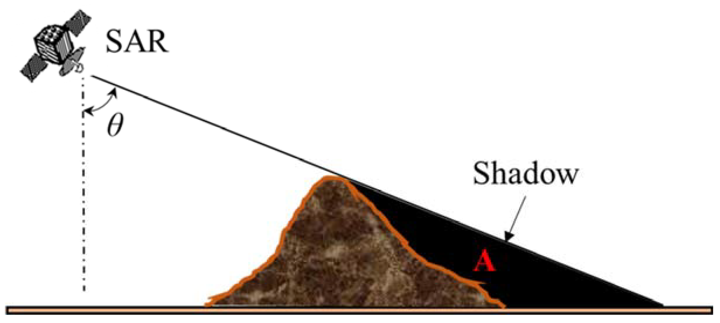
2. Shadow Formation and Expression

Shadows in SAR imagery are formed because a steep terrain or high artificial targets block electromagnetic waves from SAR to the ground surface. As shown in Figure 1, the shadow field, indicated by A, cannot be illuminated by a SAR sensor. Consequently, SAR cannot receive any backscattered echoes from the shadow field, except for system noise [35]. The shadow can be expressed as

$$Z_s=k·\eta$$

(2)

in which

$$\eta =x+i·y$$

(3)

Here, $Z_s$ denotes the values of shadows. It is usually expressed in complex form. $k$ represents the backscatter of objects in the shadow area, which is zero theoretically [35]. To avoid a zero $Z_s$ value, $k$ can be assumed to be a minimal constant close to zero. Although the shadow constant may vary with different image regions or observation conditions, each shadow formation principle is the same, and the shadow signal mainly comes from system noise. For simplicity, the constants $k$ for all shadows can be considered the same. These assumptions are reasonable because the actual values of shadows are generally not zero. Furthermore, the statistical characteristics of shadows will not be affected by the constant, in essence. η denotes the systematic noise of SAR. It is the main component of $Z_s$ and usually expressed in complex form, namely, complex speckle noise. $x,y$ are the real and imaginary components of the complex speckle noise, respectively. $i$ is the imaginary unit, $i=\sqrt{-1}$.

As mentioned above, the value $Z_s$ of the shadow is not zero because of the systematic noise of SAR. Generally speaking, in a normal SAR system, the noise level is lower than the terrain backscatter. Consequently, the value $Z_s$ of the shadow is significantly lower than that of the surroundings, and it is mainly confined to an interval close to zero. Therefore, most state-of-the-art statistical models developed for characterizing SAR images are not suitable for shadows in SAR images.

3. Statistical Modeling of Single-Look SAR Image Shadow

In this section, the objective is to deduce the statistical models of the single-look shadow intensity and single-look shadow amplitude based on the shadow expression. According to Equation (1), the value of the shadow is scaled SAR systematic noise, i.e., scaled speckle noise. As the value of the shadow is significantly lower than that of the environment, the SAR image shadow can be reasonably regarded as a homogeneous region. In other words, it can be assumed that the speckle is fully developed in the shadow. Moreover, according to the coherent SAR imaging theory [35,36], the complex speckle noise of a shadow resolution cell is synthesized by summing a series of complex systematic noise vectors in the resolution cell. Hence, the expression of the complex speckle noise of the shadow, i.e., η (in Equation (2)), can be given as

$$x+i·y={\displaystyle {\sum }_{j=1}^n(x_j+i·y_j)}$$

(4)

By combining Equations (2)–(4), the complete expression for shadows can be given as

$$Z_s=k{\displaystyle {\sum }_{j=1}^n(x_j+i·y_j)}$$

(5)

where n is the number of complex systematic noises in a resolution cell. As [16] introduced, for a large number of independent and identically distributed noises, $x$ and $y$ are independently Gaussian-distributed with a zero mean and equal variance, and the variance is ${\delta }^2$. In order to express the statistical model of the intensity and amplitude SAR image speckle noise as a standardized mathematical model, the variance is denoted by ${\sigma }^2/2$ [16], where $\sigma =\sqrt{2}\delta$. Then, the statistical models presented in [16] for characterizing the intensity and amplitude SAR image speckle noise can be directly introduced to describe the statistical characteristics of the intensity and amplitude speckle noise of SAR image shadows, respectively. Therefore, the intensity of the complex speckle noise of shadow $I_{\eta }$, defined as $I_{\eta }=x^2+y^2$, has a negative exponential distribution (NED),

$$f_{I_{\eta 1}}(I_{\eta })=\frac{1}{{\sigma }^2}·exp\left(-\frac{I_{\eta }}{{\sigma }^2}\right),I_{\eta }\ge 0$$

(6)

where the subscript “1” denotes single-look or 1-look. $f_{I_{\eta 1}}(I_{\eta })$ is the probability density function (PDF) of $I_{\eta }$. The mean of $I_{\eta }$ is $M_1(I_{\eta })={\sigma }^2$, and the variance is $Va{r}_1(I_{\eta })={\sigma }^4$.

The amplitude of the complex speckle noise of the shadow, $A_{\eta }$, defined as $\sqrt{I_{\eta }}$, has a Rayleigh distribution,

$$f_{A_{\eta 1}}\left(A_{\eta }\right)=\frac{2A_{\eta }}{{\sigma }^2}exp\left(-\frac{A_{\eta }^2}{{\sigma }^2}\right),A_{\eta }\ge 0$$

(7)

The mean is $\sigma \sqrt{\pi }/2$, and the variance is $\left(4-\pi \right){\sigma }^2/4$.

Based on Equation (5), the single-look intensity of shadow $I_s$ is $k^2$ times that of the complex speckle noise of shadow $I_{\eta }$,

$$I_s=k^2·I_{\eta }$$

(8)

Therefore, the PDF of the single-look shadow intensity, $f_{I_{S1}}\left(I_s\right)$, can be converted from Equations (6) and (8) as follows:

$$f_{I_{S1}}\left(I_s\right)=\frac{1}{k^2}·f_{I_{\eta 1}}\left(\frac{1}{k^2}{I}_s\right)$$

(9)

Then, the analytic distribution model of the single-look shadow intensity is derived as

$$f_{I_{S1}}\left(I_s\right)=\frac{1}{{\sigma }^2·k^2}·exp\left(-\frac{I_s}{{\sigma }^2·k^2}\right),I_s\ge 0$$

(10)

It can be seen that Equation (10) is a NED model with two parameters. For given SAR image shadows, $\sigma$ and $k$ are constant. Accordingly, let $\alpha =\sigma ·k$. The PDF of the single-look shadow intensity can be simplified as

$$f_{I_{S1}}\left(I_s\right)=\frac{1}{{\alpha }^2}·exp\left(-\frac{I_s}{{\alpha }^2}\right),I_s\ge 0$$

(11)

with the mean $M_1(I_s)={\alpha }^2$ and variance $Va{r}_1(I_s)={\alpha }^4$. Equations (6) and (11) are identical in form, but their parameters, $\sigma$ and $\alpha$, are not the same.

The amplitude value of the shadow, $A_s$, is the square root of the intensity value of the shadow, $A_s=\sqrt{I_s}$. According to Equation (8), $A_s$ is $k$ times that of the complex speckle noise of the shadow, $A_{\eta }$, $A_s=k{A}_{\eta }$. Therefore, the PDF of the single-look shadow amplitude, $f_{A_{S1}}\left(A_s\right)$, can be derived from Equation (7) as follows:

$$\begin{array}{ll}{f}_{A_{S1}}\left(A_s\right)& =\frac{1}{k}{f}_{A_{\eta 1}}\left(\frac{1}{k}{A}_S\right)\\ & =\frac{2A_S}{k^2·{\sigma }^2}·exp\left(-\frac{A_S^2}{k^2·{\sigma }^2}\right)\end{array}$$

(12)

Let $\alpha =\sigma ·k$. The PDF of the single-look shadow amplitude can be simplified as

$$f_{A_{S1}}\left(A_s\right)=\frac{2A_s}{{\alpha }^2}·exp\left(-\frac{A_s^2}{{\alpha }^2}\right),A_s\ge 0$$

(13)

Obviously, the single-look shadow amplitude follows a Rayleigh distribution with the mean $M_1(A_s)=\alpha \sqrt{\pi }/2$ and variance $Va{r}_1(A_s)=(4-\pi ){\alpha }^2/4$.

The form of the deduced NED and Rayleigh models for single-look SAR image shadows looks similar to the corresponding models for SAR images in [16]. This is because the deduced statistical models for shadows and the statistical models of SAR images both originate from the same speckle noise expression in Equation (4). The significant difference is that the parameter $\alpha$ of shadow models is $k$ times the parameter $\sigma$ of SAR image models.

4. Statistical Modeling of Multilook SAR Image Shadow

Multilooking is a common procedure for correcting the distortion of the azimuth and range resolution of single-look SAR images, and it also has the ability to suppress speckle noise. According to the theory of statistics, multilooking changes the statistical characteristics of the SAR image shadow. Since the SAR image is commonly expressed in complex form, multilooking can be implemented in the real domain on amplitude and intensity individually or on both real and imaginary components in the complex domain. Accordingly, the statistical characteristics of SAR image shadows multilooked in the real domain and complex domain will be different. The purpose of this section is to deduce the statistical models of SAR image shadows multilooked in the real domain and complex domain.

4.1. Modeling of SAR Image Shadow Multilooked in Real Domain

According to [19], the set of samples obtained within the full synthetic aperture can be split into several adjacent subsets. Each subset forms a separate image, namely, a 1-look image. Multilooking is to average adjacent 1-look images. It can be performed in the real domain or complex domain. For the former, the 1-look image is first converted to intensity or amplitude, and multilooking is then performed on the intensity or amplitude. Multilooking in the real domain can not only correct image distortion but also improve the radiometric accuracy of measurements, and thus, it is popular in SAR image applications.

Given an intensity SAR image multilooked in the real domain, and assuming that the shadow constants k in all 1-look images are equal, the multilook shadow intensity can be calculated with Equation (5) and expressed as

$$I_{MLR}=\frac{1}{N}{\displaystyle {\sum }_{j=1}^N{I}_s(j)=\frac{k^2}{N}{\displaystyle {\sum }_{j=1}^N\left(x{(j)}^2+y{(j)}^2\right)}}$$

(14)

where $I_{MLR}$ is the shadow intensity multilooked in the real domain. N is the multilook number. $I_s(j)$ is the intensity of the jth look. $x(j)$ and $y(j)$ are the real and imaginary parts of the $j$th look, respectively, and they are independently Gaussian-distributed with a zero mean and equal variance, i.e., $x\left(j\right),y\left(j\right)~N\left(0,\frac{{\sigma }^2}{2}\right)$. According to probability theory, $\frac{x\left(j\right)}{\sigma /\sqrt{2}}$ and $\frac{y\left(j\right)}{\sigma /\sqrt{2}}$ follow the standard normal distribution, i.e., $\frac{x\left(j\right)}{\sigma /\sqrt{2}}~N\left(0,1\right)$ and $\frac{y\left(j\right)}{\sigma /\sqrt{2}}~N\left(0,1\right)$. Therefore, the sum ${\displaystyle {\sum }_{j=1}^N\left({\left(\frac{x\left(j\right)}{\sigma /\sqrt{2}}\right)}^2+{\left(\frac{y\left(j\right)}{\sigma /\sqrt{2}}\right)}^2\right)}$ obeys a chi-square distribution with 2N degrees of freedom, i.e., ${\displaystyle {\sum }_{j=1}^N\left({\left(\frac{x\left(j\right)}{\sigma /\sqrt{2}}\right)}^2+{\left(\frac{y\left(j\right)}{\sigma /\sqrt{2}}\right)}^2\right)}~{\chi }^2\left(2N\right)$. ${\displaystyle {\sum }_{j=1}^N\left({\left(\frac{x\left(j\right)}{\sigma /\sqrt{2}}\right)}^2+{\left(\frac{y\left(j\right)}{\sigma /\sqrt{2}}\right)}^2\right)}$ can be converted to

$${\displaystyle {\sum }_{j=1}^N\left({\left(\frac{x\left(j\right)}{\sigma /\sqrt{2}}\right)}^2+{\left(\frac{y\left(j\right)}{\sigma /\sqrt{2}}\right)}^2\right)}=\frac{{\displaystyle {\sum }_{j=1}^N\left(x{\left(j\right)}^2+y{\left(j\right)}^2\right)}}{{\sigma }^2/2}$$

(15)

Let $I^{\prime }={\displaystyle {\sum }_{j=1}^N\left(x{\left(j\right)}^2+y{\left(j\right)}^2\right)}$; then, $\frac{I^{\prime }}{{\sigma }^2/2}~{\chi }^2\left(2N\right)$, and Equation (14) can be transformed into

$$I_{MLR}=\frac{k^2}{N}{I}^{\prime }$$

(16)

Therefore, the PDF of the multilook shadow intensity $I_{MLR}$ can be derived as

$$f_N(I_{MLR})={(\frac{N}{{\sigma }^2·k^2})}^N·\frac{I_{MLR}{}^{N-1}}{\mathsf{\Gamma }(N)}·exp\left(-\frac{N}{{\sigma }^2·k^2}·I_{MLR}\right),I_{MLR}\ge 0$$

(17)

with the mean $M_N(I_{MLR})={\sigma }^2·k^2$ and variance $Va{r}_N(I_{MLR})={\sigma }^4·k^4/N$. Here, $\mathsf{\Gamma }()$ is the Gamma function. By substituting $\alpha =\sigma ·k$, the PDF of the shadow intensity multilooked in the real domain is simplified as

$$f_N(I_{MLR})=\frac{N^N·I_{MLR}{}^{N-1}}{{\alpha }^{2N}·\mathsf{\Gamma }(N)}·exp\left(-\frac{N}{{\alpha }^2}·I_{MLR}\right),I_{MLR}\ge 0$$

(18)

with the mean $M_N(I_{MLR})={\alpha }^2$ and variance $Va{r}_N(I_{MLR})={\alpha }^4/N$. Obviously, the shadow intensity multilooked in the real domain follows a Gamma distribution with 2N degrees of freedom. A comparison with [16] indicates that Equation (18) and the PDF proposed in [16] for multilook intensity speckle are in the same form. The significant difference lies in the parameters $\alpha$ and $\sigma$.

The multilook shadow amplitude can be obtained in two ways. One way is to obtain it directly from the multilook amplitude SAR image. The other way is to use the square root of the multilook shadow intensity. In the former way, the analytic form of the PDF of the multilook shadow amplitude is hardly obtained. In the latter way, the multilook shadow amplitude, $A_{MLR}$ is $A_{MLR}=\sqrt{I_{MLR}}$. Accordingly, the PDF of the multilook shadow amplitude can be derived from Equation (18).

$$f_N(A_{MLR})=\frac{2N^N}{{\alpha }^{2N}·\mathsf{\Gamma }(N)}·A_{MLR}{}^{2N-1}·exp\left(-\frac{N}{{\alpha }^2}·A_{MLR}{}^2\right),A_{MLR}\ge 0$$

(19)

The mean of $A_{MLR}$ is $M_N(A_{MLR})=\alpha ·\mathsf{\Gamma }(N+\frac{1}{2})/(\mathsf{\Gamma }(N)·\sqrt{N})$, and the variance is $Va{r}_N(A_{MLR})={\alpha }^2-{\alpha }^2·{\mathsf{\Gamma }}^2(N+\frac{1}{2})/(N·{\mathsf{\Gamma }}^2(N))$. Obviously, the shadow amplitude multilooked in the real domain follows a Nakagami distribution. Similarly, the comparison with [16] indicates that Equation (19) and the PDF proposed in [16] for multilook intensity speckle are in the same form. The significant difference lies in the parameters $\alpha$ and $\sigma$. The reason is the same as described in Section 3.

4.2. Modeling of SAR Image Shadow Multilooked in Complex Domain

In addition to multilooking the SAR image in the real domain, the SAR image is sometimes multilooked in the complex domain by averaging its real and imaginary components, respectively. In this way, the multilook shadow is also complex. Its calculation formula can be derived from Equation (5) and expressed as

$$\overline{Z_s}=k\left(\frac{1}{N}{\displaystyle {\sum }_{j=1}^{N}x(j)+i·\frac{1}{N}{\displaystyle {\sum }_{j=1}^{N}y(j)}}\right)$$

(20)

where $\overline{Z_s}$ denotes the shadow multilooked in the complex domain. $x(j)$ and $y(j)$ are the real and imaginary parts of the jth look, respectively. Then, the multilook shadow intensity is given as

$$I_{MLC}=k^2\left({\left(\frac{1}{N}{\displaystyle {\sum }_{j=1}^{N}x(j)}\right)}^2+{\left(\frac{1}{N}{\displaystyle {\sum }_{j=1}^{N}y(j)}\right)}^2\right)$$

(21)

where $I_{MLC}$ is the shadow intensity multilooked in the complex domain.

Let $X\prime =\frac{1}{N}{\displaystyle {\sum }_{j=1}^{N}x(j)}$ and $Y\prime =\frac{1}{N}{\displaystyle {\sum }_{j=1}^{N}y(j)}$. We obtain

$$I_{MLC}=k^2(X{\prime }^2+Y{\prime }^2)$$

(22)

On the basis of the same assumption as Equation (14) for $x(j)$ and $y(j)$, it is easy to know that ${(\frac{X\prime }{\sigma /\sqrt{2N}})}^2+{(\frac{Y\prime }{\sigma /\sqrt{2N}})}^2$ obeys the chi-square distribution with 2 degrees of freedom, i.e., $\frac{X{\prime }^2}{{\sigma }^2/2N}+\frac{Y{\prime }^2}{{\sigma }^2/2N}~{\chi }^2\left(2\right)$. According to Equation (22), the PDF of $I_{MLC}$ can be derived as

$$f_N(I_{MLC})=\frac{N}{{\alpha }^2}·exp\left(-\frac{N}{{\alpha }^2}·I_{MLC}\right),I_{MLC}\ge 0$$

(23)

where $\alpha =\sigma ·k$. Equation (23) shows that the shadow intensity multilooked in the complex domain has a negative exponential distribution modulated by the multilook number (M-NED) with the mean $M_N(I_{MLC})={\alpha }^2/N$ and variance $Va{r}_N(I_{MLC})={\alpha }^4/N^2$.

The shadow amplitude multilooked in the complex domain, $A_{MLC}$, is the square root of the shadow intensity, i.e., $A_{MLC}=\sqrt{I_{MLC}}$. Accordingly, the PDF of the shadow amplitude multilooked in the complex domain can be easily deduced from Equation (23) as follows.

$$f_N(A_{MLC})=\frac{2N·A_{MLC}}{{\alpha }^2}·exp\left(-\frac{N·A_{MLC}^2}{{\alpha }^2}\right),A_{MLC}\ge 0$$

(24)

As shown in Equation (24), the shadow amplitude multilooked in the complex domain obeys a Rayleigh distribution modulated by the multilook number (M-Rayleigh). The mean and variance are $M_N(A_{MLC})=\sqrt{\pi /N}·\alpha /2$ and $Va{r}_N(A_{MLC})=(4-\pi )/4N{\alpha }^2$, respectively. It is obvious that there is a significant difference between the statistical models of shadows multilooked in the real domain and complex domain.

5. Modeling of Filtered SAR Image Shadow

Filtering is a common procedure for suppressing SAR image noise. It will change the statistical characteristics of the SAR image and shadow. Since each filter has its own specific algorithm, theoretically, the image filtered by a given filter has its own specific statistical model. Next, taking the classic Lee filter [37] as an example, we will demonstrate the derivation of the statistical characteristics of SAR images filtered by the Lee filter. According to [37], the formula for the Lee filter is

$${\hat{Z}}_p={\overline{Z}}_p+C(Z_p-{\overline{Z}}_p)=C·Z_p+(1-V){\overline{Z}}_p$$

(25)

where $Z_p$ and ${\hat{Z}}_p$ are the observation, i.e., intensity, and filtered output of pixel $p$, respectively. ${\overline{Z}}_p$ is the mean value of pixels within a window centered on pixel $p$. $C$ is the filtering coefficient, and it is a constant. $C·Z_p$ and $(1-C){\overline{Z}}_p$ can be regarded as two independent random variables. Let $X_1=C·Z_p$ and $X_2=(1-C){\overline{Z}}_p$; the formula for the Lee filter can be simplified as

$${\hat{Z}}_p=X_1+X_2$$

(26)

Therefore, the random variable ${\hat{Z}}_p$, i.e., the filtered output, is the sum of two independent random variables.

Since $Z_p$ follows the distribution of the single-look shadow intensity, i.e., Equation (11), the PDF of the random variable $X_1$ can be derived as

$$f_{X_1}(x_1)=\frac{1}{C{\alpha }^2}·exp\left(-\frac{x_1}{C{\alpha }^2}\right),x_1\ge 0$$

(27)

Furthermore, ${\overline{Z}}_p$ is identical to the multilook result of the filtering window centered on pixel $p$, and its distribution characteristics can be represented by the distribution of the multilook shadow intensity.

$$f({\overline{Z}}_P)=\frac{N^N·{\overline{Z}}_P{}^{N-1}}{{\alpha }^{2N}·\mathsf{\Gamma }(N)}·exp\left(-\frac{N}{{\alpha }^2}·{\overline{Z}}_P\right),{\overline{Z}}_P\ge 0$$

(28)

where $N$ is the scale of the Lee filtering window $N\times N$. Based on Equation (28), the PDF of the random variable $X_2$ can be derived as

$$f_{X_2}(x_2)={\left(\frac{N}{\left(1-C\right){\alpha }^2}\right)}^N\frac{x_2{}^{N-1}}{\mathsf{\Gamma }(N)}·exp\left(-\frac{N}{\left(1-C\right){\alpha }^2}{x}_2\right),x_2\ge 0$$

(29)

According to Equations (26), (27), and (29), the PDF of the filtered output ${\hat{Z}}_p$ can be derived as

$$\begin{array}{ll}{f}_{{\hat{Z}}_p}({\hat{z}}_p)& ={\displaystyle {\int }_0^{+\infty }{f}_{X_1}\left({\hat{z}}_p-x_2\right)}·f_{X_2}\left(x_2\right)d{x}_2\\ & ={\displaystyle {\int }_0^{+\infty }\frac{1}{C{\alpha }^2}}exp\left(-\frac{{\hat{z}}_p-x_2}{C{\alpha }^2}\right)·\left[{\left(\frac{N}{\left(1-C\right){\alpha }^2}\right)}^N\frac{x_2{}^{N-1}}{\mathsf{\Gamma }(N)}·exp\left(-\frac{N}{\left(1-C\right){\alpha }^2}{x}_2\right)\right]d{x}_2\\ & =\frac{1}{\mathsf{\Gamma }(N)C{\alpha }^2}·{\left(\frac{N}{\left(1-C\right){\alpha }^2}\right)}^N{\displaystyle {\int }_0^{+\infty }{x}_2{}^{N-1}·}exp\left(-\frac{{\hat{z}}_p-x_2}{C{\alpha }^2}-\frac{N{x}_2}{\left(1-C\right){\alpha }^2}\right)d{x}_2\end{array}$$

(30)

Obviously, it is difficult to obtain the integral of $f_{{\hat{Z}}_p}({\hat{z}}_p)$. In other words, it is difficult to obtain an analytic distribution model for the filtered SAR image shadow from the physical mechanism perspective. The same problem also exists in images filtered by other filters.

As described in Section 2, speckle noise is the main component of the shadow, and its value (intensity or amplitude) is extremely small. Correspondingly, the filtered shadow value is also extremely small. Since the generalized extreme value (GEV) distribution [37] has excellent performance in characterizing the smallest or largest values among a large set of independent and identically distributed random variables, the GEV is introduced into the modeling of the filtered SAR image shadow in this paper. For both single-look and multilook filtered shadows, the statistical model of their intensity or amplitude can be uniformly expressed as follows [38]:

$$f(\mathbb{Z})=\frac{1}{a}{\left(1+\xi ·\frac{(\mathbb{Z}-b)}{a}\right)}^{-\frac{\xi +1}{\xi }}·exp\left(-{\left(1+\xi ·\frac{(\mathbb{Z}-b)}{a}\right)}^{-\frac{1}{\xi }}\right),1+\xi ·\frac{(\mathbb{Z}-b)}{a}>0$$

(31)

where $\mathbb{Z}$ denotes the intensity or amplitude of the filtered SAR image shadow, and $f(\mathbb{Z})$ is its PDF with the scale parameter a, location parameter b, and shape parameter $\xi$. The mean is $M(\mathbb{Z})=b-a/\xi +a/\left(\xi ·\mathsf{\Gamma }(1-\xi )\right)$, and the variance is $Var(\mathbb{Z})=a^2/{\xi }^2·\left(\mathsf{\Gamma }(1-2\xi )-{\mathsf{\Gamma }}^2(1-\xi )\right)$. The unknown parameters, i.e., a, b, and $\xi$, can be estimated using a maximum likelihood estimator [39].

6. Experimental Results and Discussion

In this section, we report experiments conducted on real SAR images to validate the series of deduced models of SAR image shadows. Firstly, these deduced models were tested using the chi-square goodness-of-fit tests. Then, qualitative and quantitative comparisons were made between the deduced models of shadows and the state-of-the-art statistical models of SAR imagery. This comparison was made to evaluate the performance of these deduced models and provide suggestions for the selection of the optimal statistical model of shadows for multimodal SAR images.

6.1. Experimental Data and Scheme

Our experiments utilized a SAR image of the Nyingchi region in Tibet, acquired by TanDEM-X in December 2013 (see Figure 2). Due to the steep topography, a large number of shadows are observed in the SAR image example (e.g., outlined in green in Figure 2). Filtering and multilooking of the SAR image were implemented with the Sentinel Application Platform (SNAP) ver. 9.0.0 software. From the single-look SAR image and correspondingly filtered SAR image, 523,177 shadow pixels were automatically extracted. After the single-look SAR image was multilooked at a ratio of 2:2, 131,651 shadow pixels were obtained from the multilook SAR image in the real domain, the multilook SAR image in the complex domain, and the correspondingly filtered SAR images.

The performance of the series of deduced models was evaluated by qualitative and quantitative comparisons with state-of-the-art statistical models. It is known that SAR image shadows are almost homogeneous, and their values are extremely small. Therefore, κ, g⁰, GΓD, and GΓR distributions that can characterize the statistical characteristics of homogeneous regions (see Table 1) were chosen as references for comparison. Also, the GEV distribution was involved. The qualitative comparison is depicted by the normalized histograms of shadow samples, deduced models, and reference distributions. The quantitative comparison is illustrated by the symmetrical Kullback–Leibler (KL) distance [40] between the normalized histogram of shadow samples and the estimated PDFs of the deduced and reference distributions.

$$D_{KL}(F,P)=\frac{1}{2}{\displaystyle {\sum }_{i=0}^N(f(x_i)In\frac{f(x_i)}{p_i}+p(i)In\frac{p(i)}{f(x_i)})}$$

(32)

where $D_{KL}(F‖P)$ is the symmetrical KL distance between a statistical distribution model F and a set of samples P. $f(x_i)$ represents the probability density of the statistical distribution model F at $x_i$. $p(i)$ is the height of bin I, and N is the total number of bins in the frequency histogram of the sample. The smaller symmetric KL distance indicates better consistency between the estimated PDF and the sample data.

The validation of the GEV distribution was performed on a series of filtered multimodal SAR images. At the same time, the performance of the GEV distribution on filtered SAR image shadows was evaluated by performing qualitative and quantitative comparisons with κ, g⁰, GΓD, and GΓR distributions.

In the experiment, the parameters of the derived statistical models and GEV distribution were estimated using a maximum likelihood estimator. The parameters of GΓD and GΓR distributions were estimated with the logarithmic cumulant method [20], and the parameters of κ and g⁰ distributions were estimated using a moment estimator.

6.2. Chi-Square Goodness-of-Fit Tests of Deduced Models

In order to validate the derived models for multimodal SAR image shadows, we conducted chi-square goodness-of-fit tests on all deduced models and the GEV distribution. The test statistic values for all distributions are presented in

Table 2. Results of chi-square goodness-of-fit tests on GEV, NED, Rayleigh, Gamma, M-NED, Nakagami, and M-Rayleigh distributions. r is the number of degrees of freedom. The symbol / indicates that the statistical test was not passed.

Samples	n = 10,000		n = 20,000		n = 50,000		n = 100,000
	Chi-Square Stat	p-Value	Chi-Square Stat	p-Value	Chi-Square Stat	p-Value	Chi-Square Stat	p-Value
NED	5.7573	0.9278 (r = 12)	10.9234	0.6172 (r = 13)	17.6603	0.2809 (r = 15)	20.6354	0.1922 (r = 16)
Rayleigh	9.2035	0.6855 (r = 12)	14.8233	0.3185 (r = 13)	19.9137	0.1753 (r = 15)	21.0974	0.1748 (r = 16)
M-NED	7.7898	0.8013 (r = 12)	13.5467	0.4065 (r = 13)	16.3543	0.3589 (r = 15)	22.1802	0.1375 (r = 16)
M-Rayleigh	8.3445	0.7577 (r = 12)	10.6023	0.6441 (r = 13)	19.9641	0.1733 (r = 15)	21.3512	0.1654 (r = 16)
GEV	7.2102	0.7055 (r = 10)	9.3685	0.5879 (r = 11)	16.0199	0.2481 (r = 13)	21.0521	0.1003 (r = 14)
Gamma		/		/		/		/
Nakagami		/		/		/		/

. These tests were conducted on four groups of samples with different sizes (n = 10,000, 20,000, 50,000, 100,000), and the four groups of test samples were randomly selected from the corresponding shadow pixels, i.e., the shadow population. The number of histogram classes that were subject to the goodness-of-fit tests was determined by the Sturges rule. The number of degrees of freedom was determined by the number of histogram classes and the number of unknown parameters of the models.

As shown in Table 2, all models, except for the Gamma and Nakagami models, passed the tests with a significance level of 0.05 (α = 0.05). The test results indicate that the deduced Gamma and Nakagami distributions cannot effectively characterize the statistics of SAR image shadows multilooked in the real domain. The main reason is probably that the assumption that the summation part in Equation (14) is chi-square-distributed with 2N degrees of freedom is not completely true. A more accurate assumption is needed to deduce the physical mechanism model of this kind of SAR image shadow.

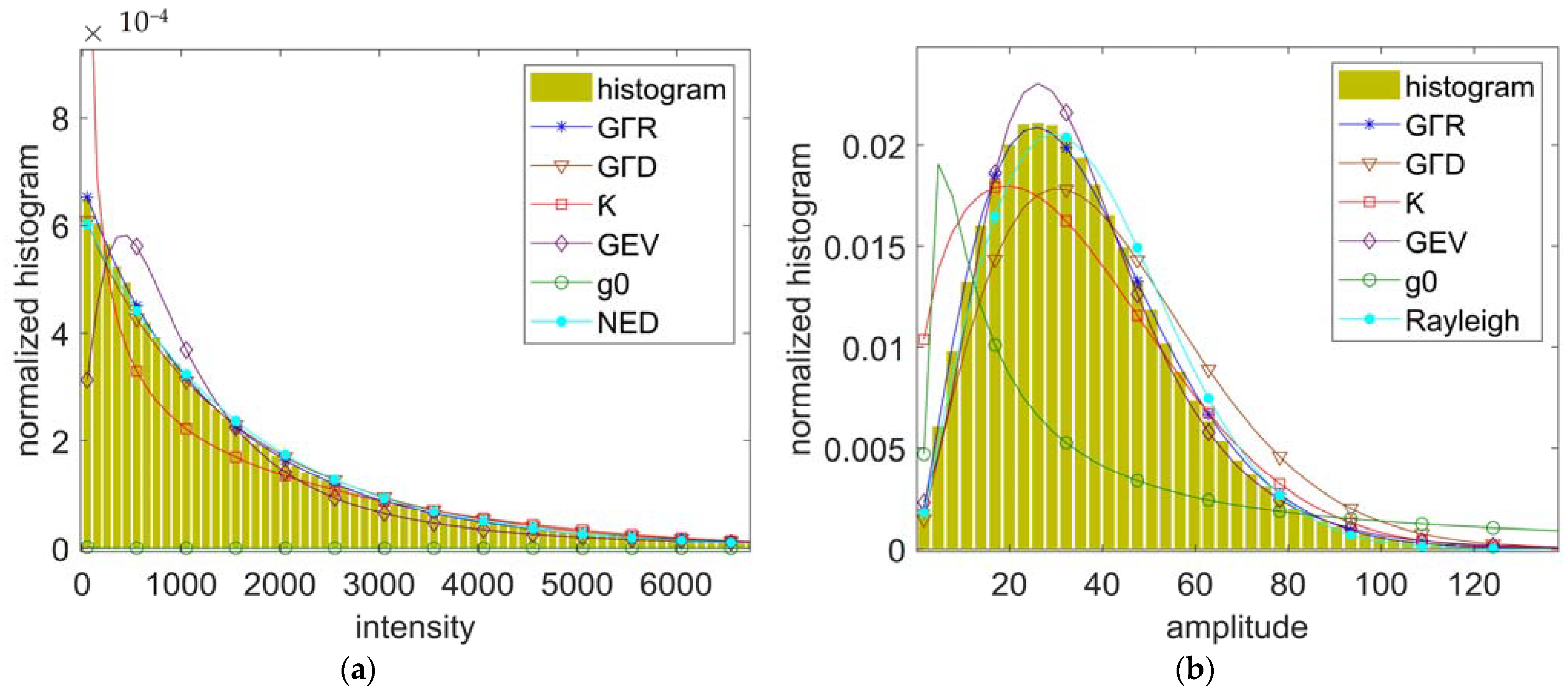
6.3. Experiment on Single-Look SAR Image Shadow

The purpose of this experiment is to evaluate the performance of Equation (11) and Equation (13), i.e., the NED distribution and Rayleigh distribution, respectively. A total of 523,177 shadow samples were used in this experiment. The estimated PDFs of the NED, Rayleigh, GΓR, GΓD, κ, g⁰, and GEV distributions are depicted in Figure 3, as well as the corresponding normalized histograms of the samples. The quantitative comparison results of all the models are shown in

Table 3. Values of symmetrical KL distance obtained by GΓR, GΓD, κ, g⁰, GEV, NED, and Rayleigh distributions. Best values are displayed in bold font.

Distribution	Intensity	Amplitude
NED	0.0000316	—
Rayleigh	—	0.0037223
GΓR	0.0000074	0.0006900
GΓD	0.0000204	0.0101596
κ	0.0004125	0.0142517
g0	0.0326374	0.1551140
GEV	0.0002549	0.0010526

.

As shown in Figure 3a, the derived NED distribution has almost the same performance as the GΓR and GΓD distributions in characterizing shadow intensity statistics, though the symmetrical KL distance value of the deduced NED model is slightly smaller than those of the GΓR and GΓD distributions (see Table 3). In Figure 3b, it can be seen that the deduced Rayleigh distribution has good performance in modeling the statistics of the shadow amplitude, though the symmetrical KL distance value of the deduced Rayleigh model is slightly smaller than that of the GΓR distribution. However, in both cases, the performance of the κ and GEV distributions is inferior to that of the deduced NED and Rayleigh distributions. And the g⁰ distribution is offset by a significant distance from the histogram. The same conclusion can also be confirmed from the visual point of view (see Figure 3).

The experimental results show that the shadow Intensity and amplitude in single-look SAR images follow the deduced NED distribution and Rayleigh distribution, respectively. In addition, the GΓR distribution can also effectively characterize the statistical characteristics of the shadow intensity and amplitude in single-look SAR images.

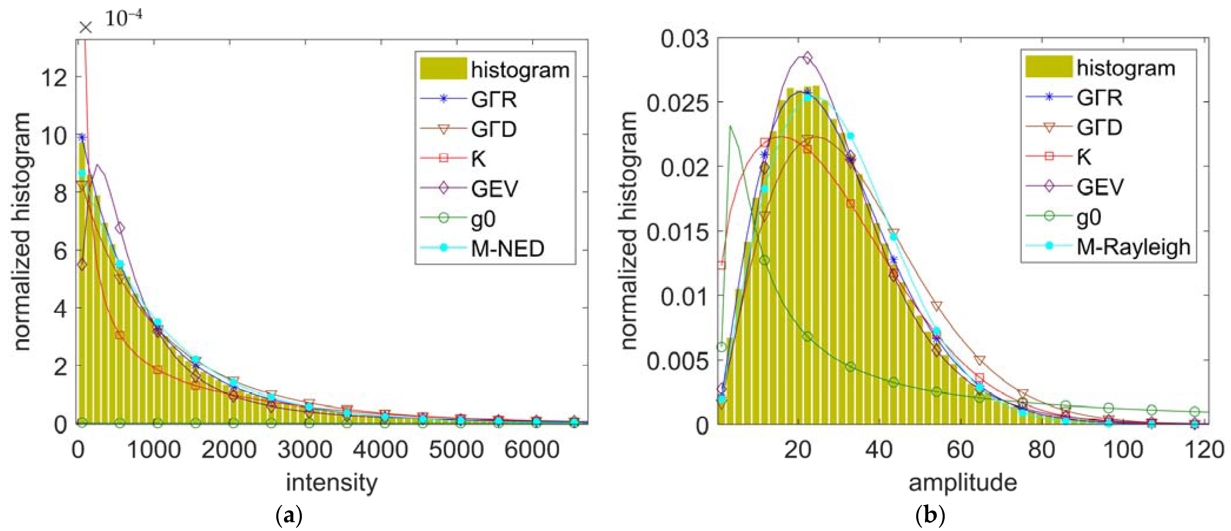
6.4. Experiment on SAR Image Shadow Multilooked in Real Domain

The goal of this experiment was to evaluate the performance of deduced Equations (18) and (19), i.e., the Gamma distribution and Nakagami distribution. The SAR image was multilooked in the real domain at a ratio of 2:2, i.e., four multilook numbers, and 131,651 shadow samples were obtained from the multilook image. The estimated PDFs of the Gamma, Nakagami, GΓR, GΓD, κ, g⁰, and GEV distributions are illustrated in Figure 4, as well as the corresponding normalized histograms of samples. The quantitative comparison results of all the models are shown in

Table 4. Values of symmetrical KL distance obtained by GΓR, GΓD, κ, g⁰, GEV, Gamma, and Nakagami distributions for 2:2 multilooked shadows. Best values are displayed in bold font. The mark “F” means the failure of the estimation of the symmetrical KL distance.

Distribution	Intensity	Amplitude
Gamma	0.000242	—
Nakagami	—	0.016177
GΓR	0.000009	0.000934
GΓD	0.562952	F
κ	0.002410	0.046220
g0	0.000610	0.009446
GEV	0.000035	0.000246

. In the table, Gamma and Nakagami denote Equations (18) and (19), respectively.

In Figure 4, it can be seen that there is a significant deviation between the probability density function curves of the deduced Gamma and Nakagami distributions and the histograms of the samples. This phenomenon coincides with the statistical test results of these two distributions, as shown in Table 2. The values of the symmetrical KL distance listed in Table 4 also indicate that the performance of the deduced Gamma and Nakagami distributions in characterizing shadow statistics is significantly inferior to that of the GΓR and GEV distributions.

Furthermore, both Figure 4 and the values of the symmetrical KL distance listed in Table 4 show that the GΓR distribution is the best model to characterize the shadow intensity of the multilook SAR image, followed by the GEV distribution. The g⁰ and κ distributions have the worst performance. The GΓD distribution has the maximum symmetrical KL distance value. For the multilook shadow amplitude, the GΓR and GEV distributions also yield a good performance in characterizing its statistics, and the g⁰ and κ distributions supply a poor performance. The maximum symmetrical KL distance of the GΓD distribution indicates that the GΓD distribution hardly fits the histogram of the multilook shadow amplitude. Therefore, in the case of the terrible performance of the deduced Gamma and Nakagami distributions in characterizing the statistics of SAR image shadows multilooked in the real domain, the GΓR and GEV distributions can be used to characterize both the intensity and amplitude SAR image shadows multilooked in the real domain.

6.5. Experiment on SAR Image Shadow Multilooked in Complex Domain

The purpose of this experiment was to evaluate the performance of Equations (23) and (24), i.e., the M-NED distribution and M-Rayleigh distribution. Like the operation in Section 6.4, the SAR image was multilooked in the complex domain at a ratio of 2:2, i.e., four multilook numbers. Also, 131,651 shadow samples were used in this experiment. The values of the symmetrical KL distance obtained by the M-NED, M-Rayleigh, GΓR, GΓD, κ, g⁰, and GEV distributions are listed in

Table 5. Values of symmetrical KL distance obtained by GΓR, GΓD, κ, g⁰, GEV, M-NED, and M-Rayleigh distributions for shadows multilooked in complex domain. Best values are displayed in bold font.

Distribution	Intensity	Amplitude
M-NED	0.000066	—
M-Rayleigh	—	0.005537
GΓR	0.000010	0.001119
GΓD	0.000127	0.014428
κ	0.000826	0.020225
g0	0.000484	0.225945
GEV	0.000234	0.000288

. The normalized histograms and the estimated PDFs for the shadow intensity and amplitude are illustrated in Figure 5. In Table 5, M-NED and M-Rayleigh represent deduced Equations (23) and (24), respectively.

We found that, in Table 5, the symmetrical KL distance value of the deduced M-NED distribution is slightly larger than that of the GΓR distribution and slightly smaller than that of the GΓD distribution, while the κ, g⁰, and GEV distributions are offset by a significant distance from the histogram. In Figure 5a, it can be seen that the deduced M-NED distribution can characterize the statistical characteristics of the shadow intensity of the SAR image multilooked in the complex domain. As for the multilook shadow amplitude, the performance of M-Rayleigh is slightly inferior to that of the GEV and GΓR distributions. As shown in Figure 5, the probability density curves of the deduced M-NED and M-Rayleigh distributions are in good agreement with the shadow histograms. Therefore, the M-NED and M-Rayleigh distributions can be used separately for the statistical modeling of the intensity and amplitude of shadows multilooked in the complex domain. Of course, the GΓR distribution can be applied to the statistical modeling of the shadow intensity and amplitude.

6.6. Experiment on Filtered SAR Image Shadow

The goal of this experiment was to validate the GEV distribution on the filtered SAR image shadow. Meanwhile, its performance was evaluated by qualitative and quantitative comparisons with GΓR, GΓD, κ, and g⁰ distributions. It has been proved in Section 6.4 that the GEV distribution can characterize the statistics of shadows multilooked in the real domain. Therefore, only the single-look SAR image and the SAR image multilooked with a ratio of 2:2 in the complex domain were used in this experiment. These images were filtered by a Lee filter with a window size of 3 × 3. The values of the symmetrical KL distance obtained by the GΓR, GΓD, κ, g⁰, and GEV distributions are listed in

Table 6. Values of symmetrical KL distance obtained by GΓR, GΓD, κ, g⁰, and GEV distributions for filtered shadow intensity and amplitude. The mark “F” means the failure of the estimation of the symmetrical KL distance of the GΓD distribution. The best values are displayed in bold font.

Image		GEV	GΓR	GΓD	κ	g0
Intensity	Single-look	0.000012	0.000054	1.682804	0.003711	0.000186
	Multilook	0.000004	0.000131	F	0.003649	0.000101
Amplitude	Single-look	0.000135	0.004880	0.202100	0.067226	0.001377
	Multilook	0.000690	0.016712	F	0.062596	0.002651

. The normalized histograms and the estimated PDFs, excluding GΓD, are illustrated in Figure 6.

As shown in Figure 6 and Table 6, all of the symmetrical KL distance values of the GEV distribution are the smallest. It is obvious that the GEV distribution is the best generic model to characterize the filtered SAR image shadow, whether for amplitude or intensity, single-look or multilook images. The probability values obtained by the GΓD distribution for filtered single-look and multilook shadow intensities are extremely small, and the estimated symmetric KL distance values are invalid. However, the symmetric KL distance in the filtered shadow amplitude is too large. Therefore, the filtered SAR image shadows do not conform to the GΓD distribution. Meanwhile, the κ distribution has the largest symmetrical KL distance values in all filtered SAR image shadows, which means that the κ distribution is not suitable for the statistical modeling of the filtered SAR image shadow. Moreover, the GΓR distribution performs poorly on the filtered shadows, except for the filtered single-look shadow intensity. The performance of the g⁰ distribution is inferior to that of the GΓR distribution. The same conclusion can be drawn by visual comparison in Figure 6.

7. Conclusions

In this study, a series of statistical models of shadows for multimodal SAR images were systematically deduced from the physical mechanism perspective. Based on a real SAR image, chi-square tests were conducted on these models. Moreover, the performance of these models in characterizing the statistical characteristics of shadows was evaluated on the real SAR image and compared qualitatively and quantitatively with GΓR, GΓD, κ, and g⁰ distributions. Based on this study, it can be concluded that the intensity and amplitude of shadows in single-look SAR images follow the derived NED distribution and Rayleigh distribution, respectively. The intensity and amplitude of shadows multilooked in the complex domain conform to the deduced M-NED distribution and M-Rayleigh distribution, respectively. The deduced Gamma distribution and Nakagami distribution for shadows multilooked in the real domain perform poorly in characterizing the statistical characteristics of such shadows. The filtered shadow intensity and amplitude obey the GEV distribution. Furthermore, the GΓR distribution performs well in characterizing the statistical characteristics of shadow intensity and amplitude in multimodal SAR images, except for filtered shadows. The research results of this article can provide a reference for the selection of the optimal statistical model for shadows in multimodal SAR images in applications.

Although statistical models for shadows in multimodal SAR images have been derived, the deduced Gamma and Nakagami distributions cannot effectively characterize the statistics of SAR image shadows multilooked in the real domain. Fortunately, the GΓR and GEV distributions can be used for this situation. In addition, there is still no unified statistical shadow model applicable to all types of SAR images. A generalized statistical shadow model suitable for all SAR images is worthy of future research. Furthermore, these models are derived based on the principle of coherent SAR imaging. Due to the completely different imaging principles and shadow signal compositions between SAR images and optical images, theoretically, the shadow statistical model derived in this paper is not applicable to optical images. Of course, further experiments are needed to verify this. Moreover, the derivation of statistical models for SAR image shadows in this article can provide inspiration for studying statistical models of optical image shadows and distortions in SAR images, such as layover and foreshortening. These will be our next research interests.

References

1. Papson, S.; Narayanan, R.M. Classification via the shadow region in SAR imagery. IEEE Trans. Aero. Elec. Syst. 2012, 48, 969–980. [Google Scholar] [CrossRef]
2. Gao, F.; You, J.; Wang, J.; Sun, J.; Yang, E.; Zhou, H. A novel target detection method for SAR images based on shadow proposal and saliency analysis. Neurocomputing 2017, 267, 220–231. [Google Scholar] [CrossRef]
3. Li, H.; Yu, X.; Tang, Y.; Wang, X. Shadow detection in SAR images based on greyscale distribution, a saliency model, and geometrical matching. Int. J. Remote Sens. 2020, 41, 7446–7471. [Google Scholar] [CrossRef]
4. Xu, H.; Yang, Z.; Tian, M.; Sun, Y.; Liao, G. An extended moving target detection approach for high-resolution multichannel SAR-GMTI systems based on enhanced shadow-aided decision. IEEE Trans. Geosci. Remote Sens. 2017, 56, 715–729. [Google Scholar] [CrossRef]
5. Shang, S.; Wu, F.; Zhou, Y.; Liu, Z. Moving Target Velocity Estimation of Video SAR Based on Shadow Detection. In Proceedings of the 2020 Cross Strait Radio Science and Wireless Technology Conference (CSRSWTC), Fuzhou, China, 13–16 December 2020; pp. 1–3. [Google Scholar] [CrossRef]
6. Zhong, C.; Zhang, Y.; Ding, J. A Shadow-based Method for Moving Target Detection in Video SAR. In Proceedings of the EUSAR 2021, 13th European Conference on Synthetic Aperture Radar, Online, 29 March–1 April 2021; pp. 1–6. [Google Scholar]
7. Zhao, B.; Han, Y.; Wang, H.; Tang, L.; Liu, X.; Wang, T. Robust shadow tracking for video SAR. IEEE Geosci. Remote Sens. Lett. 2020, 18, 821–825. [Google Scholar] [CrossRef]
8. Lin, Y.; Zhang, H.; Li, G.; Wang, T.; Wan, L.; Lin, H. Improving impervious surface extraction with shadow-based sparse representation from optical, SAR, and LiDAR data. IEEE J. Sel. Topic. Applic. Earth. Observ. Remote Sens. 2019, 12, 2417–2428. [Google Scholar] [CrossRef]
9. Lin, Y.; Zhang, H.; Ma, P.; Li, Y. Multisource Shadow-Based Fuzzy Set (MSFS) Approach for Impervious Surfaces Mapping from Optical and SAR Data. In Proceedings of the 2021 IEEE International Geoscience and Remote Sensing Symposium (IGARSS), Brussels, Belgium, 11–16 July 2021; pp. 6817–6820. [Google Scholar] [CrossRef]
10. Bouvet, A.; Mermoz, S.; Ballère, M.; Koleck, T.; Le Toan, T. Use of the SAR shadowing effect for deforestation detection with Sentinel-1 time series. Remote Sens. 2018, 10, 1250. [Google Scholar] [CrossRef]
11. Zhang, Y.; Meng, X.M.; Dijkstra, T.A.; Jordan, C.J.; Chen, G.; Zeng, R.Q.; Novellino, A. Forecasting the magnitude of potential landslides based on InSAR techniques. Remote Sens. Environ. 2020, 241, 111738. [Google Scholar] [CrossRef]
12. Guo, R.; Li, S.; Chen, Y.N.; Li, X.; Yuan, L. Identification and monitoring landslides in Longitudinal Range-Gorge Region with InSAR fusion integrated visibility analysis. Landslides 2021, 18, 551–568. [Google Scholar] [CrossRef]
13. Cumming, I.G.; Wong, F.H. Digital Processing of Synthetic Aperture Radar Data: Algorithms and Implementation; Artech House, Inc.: Norwood, MA, USA, 2005. [Google Scholar]
14. Gao, G. Statistical modeling of SAR images: A survey. Sensors 2010, 10, 775–795. [Google Scholar] [CrossRef]
15. Frery, A.C.; Muller, H.J.; Yanasse, C.D.C.F.; Sant’Anna, S.J.S. A model for extremely heterogeneous clutter. IEEE Trans. Geosci. Remote Sens. 1997, 35, 648–659. [Google Scholar] [CrossRef]
16. Lee, J.S.; Hoppel, K.; Mango, S.A. Unsupervised estimation of speckle noise in radar images. Int. J. Imaging Syst. Technol. 1992, 4, 298–305. [Google Scholar] [CrossRef]
17. Goodman, J.W. Some fundamental properties of speckle. J. Opt. Soc. Amer. 1976, 66, 1145–1150. [Google Scholar] [CrossRef]
18. Delignon, Y.; Pieczynski, W. Modeling non-Rayleigh speckle distribution in SAR images. IEEE Trans. Geosci. Remote Sens. 2002, 40, 1430–1435. [Google Scholar] [CrossRef]
19. Oliver, C.; Quegan, S. Understanding Synthetic Aperture Radar Images; SciTech Publishing: Raleigh, NC, USA, 2004. [Google Scholar]
20. Li, H.C.; Hong, W.; Wu, Y.R.; Fan, P.Z. An efficient and flexible statistical model based on generalized gamma distribution for amplitude SAR images. IEEE Trans. Geosci. Remote Sens. 2010, 48, 2711–2722. [Google Scholar] [CrossRef]
21. Jakeman, E. On the statistics of K-distributed noise. J. Phys. A Math. Gen. 1980, 13, 31–48. [Google Scholar] [CrossRef]
22. Chitroub, S.; Houacine, A.; Sansal, B. Statistical characterisation and modelling of SAR images. Signal Proc. 2002, 82, 69–92. [Google Scholar] [CrossRef]
23. Moser, G.; Zerubia, J.; Serpico, S.B. SAR amplitude probability density function estimation based on a generalized Gaussian model. IEEE Trans. Image Proc. 2006, 15, 1429–1442. [Google Scholar] [CrossRef] [PubMed]
24. Li, H.C.; Hong, W.; Wu, Y.R.; Fan, P.Z. On the empirical-statistical modeling of SAR images with generalized gamma distribution. IEEE J. Sel. Topic. Sig. Proc. 2011, 5, 386–397. [Google Scholar] [CrossRef]
25. Trunk, G.V.; George, S.F. Detection of targets in non-Gaussian sea clutter. IEEE Trans. Aero. Elec. Sys. 1970, 6, 620–628. [Google Scholar] [CrossRef]
26. Schleher, D.C. Radar detection in Weibull clutter. IEEE Trans. Aero. Elec. Sys. 1976, 12, 736–743. [Google Scholar] [CrossRef]
27. Tison, C.; Nicolas, J.M.; Tupin, F.; Maître, H. A new statistical model for Markovian classification of urban areas in high-resolution SAR images. IEEE Trans. Geosci. Remote Sens. 2004, 42, 2046–2057. [Google Scholar] [CrossRef]
28. Duda, R.O.; Hart, P.E.; Stork, D.G. Pattern Classification, 2nd ed.; Wiley: New York, NY, USA, 1997. [Google Scholar]
29. Peng, S.; Qu, C.; Li, J. Improved kN Nearest Neighbor Estimation Algorithm for SAR Image Clutter Statistical Modeling. In Proceedings of the 2019 4th International Conference on Information Systems Engineering (ICISE), Shanghai, China, 4–6 May 2019; pp. 87–90. [Google Scholar] [CrossRef]
30. Bruzzone, L.; Marconcini, M.; Wegmuller, U.; Wiesmann, A. An advanced system for the automatic classification of multitemporal SAR images. IEEE Trans. Geosci. Remote Sens. 2004, 42, 1321–1334. [Google Scholar] [CrossRef]
31. Mantero, P.; Moser, G.; Serpico, S.B. Partially supervised classification of remote sensing images through SVM-based probability density estimation. IEEE Trans. Geosci. Remote Sens. 2005, 43, 559–570. [Google Scholar] [CrossRef]
32. Tipping, M.E. Sparse Bayesian learning and the relevance vector machine. J. Mach. Learn. Res. 2001, 1, 211–244. [Google Scholar]
33. McLachlan, G.J.; Peel, D. Finite Mixture Models; Jon & Son: New York, NY, USA, 2000. [Google Scholar]
34. Huang, S.; Zebker, H.A. SAR Image Statistics by Bandwidth Using a Mixture Distribution of Persistent Scatterer and Clutter Distributions. In Proceedings of the 2019–2019 IEEE International Geoscience and Remote Sensing Symposium (IGARSS), Yokohama, Japan, 28 July–2 August 2019; pp. 2965–2968. [Google Scholar] [CrossRef]
35. Lee, J.S.; Pottier, E. Polarimetric Radar Imaging: From Basics to Applications; CRC Press: Boca Raton, FL, USA, 2017. [Google Scholar]
36. Curlander, J.C.; McDonough, R.N. Synthetic Aperture Radar; Wiley: New York, NY, USA, 1991; Volume 11. [Google Scholar]
37. Lee, J.S. Digital image enhancement and noise filtering by use of local statistics. IEEE Trans. Pattern Anal. Mach. Intell. 1980, 2, 165–168. [Google Scholar] [CrossRef]
38. Kotz, S.; Nadarajah, S. Extreme Value Distributions: Theory and Applications; World Scientific: Singapore, 2000. [Google Scholar]
39. El Adlouni, S.; Ouarda, T.B.; Zhang, X.; Roy, R.; Bobée, B. Generalized maximum likelihood estimators for the nonstationary generalized extreme value model. Water Resour. Res. 2007, 43, 1–13. [Google Scholar] [CrossRef]
40. MartÍnez-UsÓMartinez-Uso, A.; Pla, F.; Sotoca, J.M.; García-Sevilla, P. Clustering-based hyperspectral band selection using information measures. IEEE Trans. Geosci. Romote Sens. 2007, 45, 4158–4171. [Google Scholar] [CrossRef]
Figure 1. Schematic diagram of shadow formation. Area A represents a shadow area. θ is the look angle.
Mathematics 11 04437 g001
Figure 2. Single-look amplitude SAR image of TanDEM-X (size: 4978 × 4978 pixels; resolution: 16 m × 16 m) and shadows in research region. The green polygons are shadows. The bottom image is an enlarged view of the red dashed area in the top image.
Mathematics 11 04437 g002
Figure 3. Histograms and the estimated PDFs of shadow intensity and amplitude of single-look SAR image. (a) The PDF of shadow intensity and (b) the PDF of shadow amplitude.
Mathematics 11 04437 g003
Figure 4. Histograms and the estimated PDFs of shadow intensity and amplitude in 2:2 multilooked SAR image. (a) The PDF of shadow intensity and (b) the PDF of shadow amplitude.
Mathematics 11 04437 g004
Figure 5. Histograms and the estimated PDFs of shadow intensity and amplitude of SAR image multilooked in complex domain. (a) The PDF of shadow intensity and (b) the PDF of shadow amplitude.
Mathematics 11 04437 g005
Figure 6. Histograms and the estimated PDFs of filtered intensity and amplitude of SAR image shadows. (ad) The PDFs of filtered SAR image shadow in single-look intensity and amplitude and 2:2 multilooked intensity and amplitude in complex domain in turn.
Mathematics 11 04437 g006