Stabilization of the GLV System with Asymptotically Unbounded External Disturbances

Abstract

This paper investigates the stabilization of the generalized Lotka–Volterra (GLV) biological model, which is affected by the asymptotically unbounded external disturbances, and presents some new results. Firstly, two stabilizers are proposed for the nominal GLV system. Then, some appropriate filters are designed and applied to asymptotically track the corresponding disturbances. Based on these filters, two disturbance-estimator (DE)-based controllers are presented to cancel the corresponding disturbances. Compared to the existing results, the advantage of this paper is in handling the asymptotically unbounded external disturbances effectively. Finally, the correctness and effectiveness of the proposed results are verified by computer simulation.

1. Introduction

The chaotic system, which is named the Lorenz system [1], was first found and proven asthe classical chaotic attractor in 1963. It is well known that a chaotic system has complicated dynamical behaviors that depend sensitively on tiny variations of the initial conditions and has bounded trajectories in the phase space. Thus, chaos has been intensively studied over the past few decades because it is one of the most-fascinating phenomena in nonlinear dynamical systems. From then on, since the concepts of chaos control [2] and complete synchronization [3,4] were put forward in the 1990s, chaotic systems and the relative control problems have aroused great interest among many scholars in many disciplines and in several scientific fields. As one of the important problems of chaos control, chaos stabilization has great application potential in many fields; see [4,5,6,7,8,9] and the references therein. The stabilization of a given chaotic system refers to the fact that the orbits of the chaotic systems starting from non-zero initial conditions gradually tend to the origin under the action of the designed controller. As we know that the complete synchronization of two chaotic systems is actually the stabilization of their error (between the master system and the salve systems) under the action of a controller, the stabilization problem is the most-fundamental control problem. Therefore, for a given chaotic system, it is very important to achieve the stabilization of such a system first.

Chaotic systems are notoriously sensitive to external disturbances. Therefore, it is difficult for chaotic systems with external disturbances to achieve stabilization. At present, some achievements have been made in the study of the synchronization of chaotic systems with external disturbances; see [10,11,12,13,14] and the references therein. Among these methods, the uncertainty- and disturbance-estimator (UDE)-based control method [12,13,14] is effective at dealing with the uncertainty and disturbance. But, there are still many challenges and problems to be solved. For example, the external perturbation is usually assumed to be bounded, and its boundary is usually very small. This leads to the fact that the proposed results are too conservative in some cases. In recent years, the DE-based method [15] has been shown to be an improvement of the UDE-based method; it has shown some advantages in handling some asymptotically unbounded external disturbances. But, for some asymptotically unbounded external disturbances, such as $(A_2{t}^2+A_{1}t+A_0)e^{at}$, where $A_0,A_1,A_2$ are unknown constants, whereas a is a small known constant, there is still a lack of effective handling methods, even for the feedback based on deep reinforcement learning [16,17,18]. Thus, handling such asymptotically unbounded external disturbances has remained very challenging, which drove our current work.

On the other hand, in population dynamics, interactions are often modeled as a density-dependent functional response to growth rates. Currently, the most-influential is the GLV biological model consisting of three species. In the 1940s, Lotka and Volterra, respectively, proposed models to describe inter-species competition, which laid the theoretical basis for inter-species competition. In 1988, Samardzija and Greller proved that GLV systems [19] have a chaotic behavior, and they have multiple limit cycles for three-dimensional Lotka–Volterra systems [20]. Recently, the Lotka–Volterra equation [21] has been shown to represent a well-studied system in which two species interact as predators and prey. Some interesting results about the GLV systems have been published; see [22,23,24]. As mentioned above, the existing results are obtained assuming that the system is not subject to external disturbances. However, as we know, external disturbance cannot be completely avoided. In other words, if the GLV system is affected by external disturbances, especially for some asymptotically unbounded external disturbances, the above-obtained results are invalid. Therefore, we shall investigate the stabilization of GLV systems by extending the existing DE-based control method and present some new interesting results.

Motivated by the above discussion, the stabilization of the GLV system affected by the asymptotically unbounded external disturbances was investigated extensively in two steps. In the first step, two stabilizers are proposed for the nominal system. Some appropriate filters were designed and applied to asymptotically estimate the corresponding disturbances. Based on these filters, two DE-based controllers are presented to cancel the corresponding external disturbances in the second step. Comparing to existing results, the biggest advantage of this paper is that it deals with asymptotically unbounded external disturbances. The main contributions of this paper are summarized as follows:

I. 

The stabilization of the controlled nominal GLV system is realized by two single input controllers ($U_c$): a dynamic feedback controller and a nonlinear feedback controller;

II. 

Three suitable filters are proposed to asymptotically estimate the corresponding unbounded disturbances, and then, the corresponding disturbance estimators ($U_D$) are presented;

III. 

Two DE-based controllers ($U=U_c+U_D$) are proposed and used to achieve the stabilization of the GLV system.

The structure of this paper is as follows. Section 2 presents the the problem formulation. Section 3 lists the main results of the paper. Section 4 provides the computer simulation results. The conclusions are given in Section 5.

Before ending this section, some notations used in this paper are presented. The Laplace transform is expressed by “ℓ”; “${\mathcal{\ell }}^{-1}$” stands for the inverse Laplace transform. “∗” represents the convolution of two functions, that is

$$G\left(s\right)=\mathcal{\ell }\left[g\left(t\right)\right]={\int }_0^{+\infty }g\left(t\right)e^{-st}dt,$$

where s is a complex variable with $\mathrm{Re}\left(s\right)>0$, $g\left(t\right)$ is a function that meets some appropriate conditions, and $g\left(t\right)={\mathcal{\ell }}^{-1}\left[G\left(s\right)\right]$.

“∗” represents the convolution of two functions, that is

$$g_1\left(t\right)\ast g_2\left(t\right)={\int }_0^t{g}_1(t-\tau )g_2\left(\tau \right)d\tau$$

where $g_1\left(t\right)$ and $g_2\left(t\right)$ are some functions that meet certain conditions.

2. Problem Formulation

Consider the following controlled GLV system, which is affected by the asymptotically external disturbances:

$$\begin{array}{c}\hfill {\dot{x}}_c=f\left(x_c\right)+BU+D\left(t\right)\end{array}$$

(1)

where $x_c\in R^3$ is the state, $f\left(x_c\right)\in R^3$ is a continuous vector function, $B\in R^{3\times 1}$ is a known constant vector, $U=U_c+U_D\in R^1$ is the controller to be designed, and $D\left(t\right)$ is the unpredictable external disturbance, i.e.,

$$\begin{array}{c}\hfill f\left(x_c\right)=\left(\begin{array}{c}{f}_1\left(x_c\right)\hfill \\ f_2\left(x_c\right)\hfill \\ f_3\left(x_c\right)\hfill \end{array}\right)=\left(\begin{array}{c}{x}_{c_1}-x_{c_1}{x}_{c_2}+2x_{c_1}^2-2.9851x_{c_1}^2{x}_{c_3}\hfill \\ -x_{c_2}+x_{c_1}{x}_{c_2}\hfill \\ -3x_{c_3}+2.9851x_{c_1}^2{x}_{c_3}\hfill \end{array}\right)\end{array}$$

(2)

$$B=\left(\begin{array}{c}1\hfill \\ 0\hfill \\ 0\hfill \end{array}\right),D\left(t\right)=\left(\begin{array}{c}{D}_1\left(t\right)\hfill \\ D_2\left(t\right)\hfill \\ D_3\left(t\right)\hfill \end{array}\right)=\left(\begin{array}{c}(A_2{t}^2+A_{1}t+A_0)e^{at}\hfill \\ 0\hfill \\ 0\hfill \end{array}\right).$$

(3)

$A_0,A_1,A_2$ are unknown constants, and a is a small known constant.

If $D\left(t\right)\equiv 0$, the system (1) becomes

$$\begin{array}{c}\hfill {\dot{x}}_c=f\left(x_c\right)+B{U}_c=F(x_c,U_c)\end{array}$$

(4)

and it is usually called the nominal system, where $U_c$ is the desired controller given in Equation (1).

If $U=D\left(t\right)\equiv 0$, then the system (1) is written as follows:

$$\begin{array}{c}\hfill {\dot{x}}_c=f\left(x_c\right)=\left(\begin{array}{c}{f}_1\left(x_c\right)\hfill \\ f_2\left(x_c\right)\hfill \\ f_3\left(x_c\right)\hfill \end{array}\right)=\left(\begin{array}{c}{x}_{c_1}-x_{c_1}{x}_{c_2}+2x_{c_1}^2-2.9851x_{c_1}^2{x}_{c_3}\hfill \\ -x_{c_2}+x_{c_1}{x}_{c_2}\hfill \\ -3x_{c_3}+2.9851x_{c_1}^2{x}_{c_3}\hfill \end{array}\right)\end{array}$$

(5)

It was described extensively in [21].

The main purpose of this paper is to propose two controllers $U=U_c+U_D$ to stabilize the system (1), i.e., to realize the following performance:

$$\underset{t\to +\infty }{lim}\parallel x_c\left(t\right)\parallel =0$$

where $U_c$ is the stabilizer for the nominal system (4), i.e., the controlled system: ${\dot{x}}_c=f\left(x_c\right)+B{U}_c$ is asymptotically stable with respect to the origin, and the DE-based controller $U_D$ meets the following condition:

$$\begin{array}{c}B{U}_D=-\widehat{D}\left(t\right)\to -D\left(t\right),t\to \infty \hfill \end{array}$$

(6)

Based on the DE-based control method, this paper studied the stabilization problem of the GLV system (1) and presents some interesting results.

3. Main Result

3.1. Stabilization of the Nominal GLV System

Firstly, a dynamic gain feedback controller is proposed to achieve the stabilization of the nominal GLV system, and the conclusion is obtained as follows.

Theorem 1. 

Consider the controlled nominal system (4). The dynamic gain feedback controller $U_c$ is presented as

$$U_c=k\left(t\right)x_{c_1}$$

(7)

and

$$\dot{k}\left(t\right)=-{\Vert x_c\Vert }^2$$

(8)

Proof. 

Note that, if $x_{c_1}=0$, then the following two-dimensional subsystem:

$$\begin{array}{c}{\dot{x}}_{c_2}=-x_{c_2}\hfill \\ {\dot{x}}_{c_3}=-3x_{c_3}\hfill \end{array}$$

(9)

is asymptotically stable with respect to the origin; thus, the controlled nominal system (4) is controllable. According to the results in [5], the conclusion is obtained, which finishes the proof. □

Theorem 2. 

Consider the controlled nominal system (4). A single input nonlinear controller $U_c$ is designed as follows:

$$U_c=-101x_{c_1}+x_{c_1}{x}_{c_2}-2x_{c_1}^2+2.9851x_{c_1}^2{x}_{c_3}$$

(10)

Proof. 

Substituting the controller (10) into the system (4) yields

$$\begin{array}{c}{\dot{x}}_{c_1}=-100x_{c_1}\hfill \\ {\dot{x}}_{c_2}=-x_{c_2}+x_{c_1}{x}_{c_2}\hfill \\ {\dot{x}}_{c_3}=-3x_{c_3}+2.9851x_{c_1}^2{x}_{c_3}\hfill \end{array}$$

(11)

The coefficient matrix of the system (11) is

$$\begin{array}{c}\hfill M=\left[\begin{array}{ccc}-100\hfill & 0\hfill & 0\hfill \\ x_{c_1}\hfill & -1\hfill & 0\hfill \\ 2.9851x_{c_1}{x}_{c_3}\hfill & 0\hfill & -3\hfill \end{array}\right]\end{array}$$

(12)

Since the eigenvalues of M are $-100,-1,-3$ regardless of the value of $x_c$, so the the system (4) is asymptotically stable, which finishes the proof. □

3.2. Filters’ Design

Theorem 3. 

For the disturbance in the following form:

$$D_1\left(t\right)=A{e}^{at}$$

(13)

where $a>0$ is a known constant, yet A is an unknown constant, a suitable filter is presented as

$$G_f\left(s\right)=\frac{k}{s+(k-a)}$$

(14)

where $k\gg a>0$, and meets the following performance:

$${\widehat{D}}_1\left(t\right)=D_1\left(t\right)\ast g_f\left(t\right)=D_1\left(t\right)\ast {\mathcal{\ell }}^{-1}\left[G_f\left(s\right)\right]\to D_1\left(t\right),ast\to \infty .$$

(15)

Proof. 

Since

$$\begin{array}{c}{g}_f\left(t\right)={\mathcal{\ell }}^{-1}\left[G_f\left(s\right)\right]=k{e}^{-(k-a)t}\hfill \end{array}$$

(16)

it is concluded that

$$\begin{array}{ccc}{D}_1\left(t\right)\ast g_f\left(t\right)\hfill & =\hfill & A{e}^{at}\ast \left[k{e}^{-(k-a)t}\right]\hfill \\ \\ \hfill & =\hfill & Ak{\int }_0^t{e}^{a\tau }{e}^{-(k-a)(t-\tau )}ds\hfill \\ \\ \hfill & =\hfill & Ak{e}^{-(k-a)t}{\int }_0^t{e}^{k\tau }ds\hfill \\ \\ \hfill & =\hfill & A{e}^{-(k-a)t}[e^{kt}-1]\hfill \\ \\ \hfill & =\hfill & A{e}^{at}[1-e^{-kt}]\hfill \\ \\ \hfill & \to \hfill & D_1\left(t\right),ast\to \infty .\hfill \end{array}$$

(17)

□

Theorem 4. 

For the disturbance in the following form:

$$D_1\left(t\right)=A_2{t}^2+A_{1}t+A_0$$

(18)

where $A_2\ne 0,A_1,A_0$ are unknown constants, a suitable filter is designed as

$$G_f\left(s\right)=\frac{2s^4+12s^3+32s^2+32s+16}{s^5+7s^4+20s^3+32s^2+32s+16}$$

(19)

and meets the following performance:

$${\widehat{D}}_1\left(t\right)=D_1\left(t\right)\ast g_f\left(t\right)=D_1\left(t\right)\ast {\mathcal{\ell }}^{-1}\left[G_f\left(s\right)\right]\to D_1\left(t\right),ast\to \infty .$$

(20)

Proof. 

Since

$$\begin{array}{ccc}{g}_f\left(t\right)\hfill & =\hfill & {\mathcal{\ell }}^{-1}\left[G_f\left(s\right)\right]\hfill \\ \\ \hfill & =\hfill & \frac{1}{4}{e}^{-2t}-t{e}^{-2t}+2t^2{e}^{-2t}+\frac{7}{4}{e}^{-\frac{t}{2}}cos\left(\frac{\sqrt{7}}{2}t\right)+\frac{3\sqrt{7}}{196}sin\left(\frac{\sqrt{7}}{2}t\right)\hfill \end{array}$$

(21)

we obtain

$$\begin{array}{ccc}{D}_1\left(t\right)\ast g_f\left(t\right)\hfill & =\hfill & (A_2{t}^2+A_{1}t+A_0)\ast \hfill \\ \\ \hfill & \hfill & \left[\frac{1}{4}{e}^{-2t}-t{e}^{-2t}+2t^2{e}^{-2t}+\frac{7}{4}{e}^{-\frac{t}{2}}cos\left(\frac{\sqrt{7}}{2}t\right)+\frac{3\sqrt{7}}{196}sin\left(\frac{\sqrt{7}}{2}t\right)\right]\hfill \\ \\ \hfill & =\hfill & A_2{t}^2+A_{1}t+A_0-e^{-2t}\left(\frac{19}{16}{A}_2-\frac{9}{16}{A}_1+\frac{3}{8}{A}_0\right)\hfill \\ \\ \hfill & \hfill & -t{e}^{-2t}\left(\frac{5}{4}{A}_2-\frac{3}{4}{A}_1+\frac{1}{2}{A}_0\right)-\frac{1}{2}{t}^2{e}^{-2t}(A_2-A_1+2A_0)\hfill \\ \\ \hfill & \hfill & -\frac{1}{7}{e}^{-\frac{t}{2}}\left[cos\left(\frac{\sqrt{7}}{2}t\right)+2\sqrt{7}sin\left(\frac{\sqrt{7}}{2}t\right)\left(\frac{9A_2+5A_1-14A_0}{19A_2-9A_1-10A_0}\right)\right]\hfill \\ \\ \hfill & \to \hfill & A_2{t}^2+A_{1}t+A_0=D_1\left(t\right),ast\to \infty \hfill \end{array}$$

(22)

So, the presented filter $G_f\left(s\right)$ meets the requirements. □

Theorem 5. 

For the disturbance in the following form:

$$D_1\left(t\right)=(A_2{t}^2+A_{1}t+A_0)e^{at}$$

(23)

where $a>0$ is a known constant, yet $A_2\ne 0,A_1,A_0$ are unknown constants, a suitable filter $G_f\left(s\right)$ is presented as follows:

$$G_f\left(s\right)=\frac{a_4{s}^4+a_3{s}^3+a_2{s}^2+a_{1}s+a_0}{b_5{s}^5+b_4{s}^4+b_3{s}^3+b_2{s}^2+b_{1}s+b_0}$$

(24)

where

$$\begin{array}{c}{a}_4=-20\hfill \\ \\ a_3=80a-840\hfill \\ \\ a_2=-120a^2+2520a-9320\hfill \\ \\ a_1=80a^3-2520a^2+18640a-10400\hfill \\ \\ a_0=-20a^4+840a^3-9320a^2+10400a-16000\hfill \end{array}$$

(25)

and

$$\begin{array}{c}{b}_5=-1\hfill \\ \\ b_4=5a-61\hfill \\ \\ b_3=-10a^2+244a-1262\hfill \\ \\ b_2=10a^3-366a^2+3786a-9320\hfill \\ \\ b_1=-5a^4+244a^3-3786a^2+18640a-10400\hfill \\ \\ b_0=a^5-61a^4+1262a^3-9320a^2+10400a-16000\hfill \end{array}$$

(26)

and meets the following performance:

$${\widehat{D}}_1\left(t\right)=D_1\left(t\right)\ast g_f\left(t\right)=D_1\left(t\right)\ast {\mathcal{\ell }}^{-1}\left[G_f\left(s\right)\right]\to D_1\left(t\right),ast\to \infty .$$

(27)

Proof. 

Since

$$\begin{array}{c}{g}_f\left(t\right)={\mathcal{\ell }}^{-1}\left[G_f\left(s\right)\right]=c_2{t}^2+c_{1}t+c_0\hfill \end{array}$$

(28)

where

$$\begin{array}{c}{c}_2=\frac{4000}{191}{e}^{(a-20)t}\hfill \\ \\ c_1=\frac{690800}{36481}{e}^{(a-20)t}\hfill \\ \\ c_0=\frac{138930860}{6967871}{e}^{(a-20)t}+\frac{426560}{6967871}{e}^{(a-\frac{1}{2})t}\left[cosh\left(\frac{\sqrt{7}i}{2}t\right)+\frac{45165\sqrt{7}i}{74648}sinh\left(\frac{\sqrt{7}i}{2}t\right)\right]\hfill \end{array}$$

(29)

we obtain

$$\begin{array}{ccc}{D}_1\left(t\right)\ast g_f\left(t\right)\hfill & =\hfill & (A_2{t}^2+A_{1}t+A_0)e^{at}\ast \left(c_2{t}^2+c_{1}t+c_0\right)\hfill \\ \\ \hfill & =\hfill & A_2{t}^2{e}^{at}+A_{1}t{e}^{at}+A_0{e}^{at}+d_2{t}^2+d_{1}t+d_0\hfill \\ \\ \hfill & =\hfill & (A_2{t}^2+A_{1}t+A_0)e^{at}+d_2{t}^2+d_{1}t+d_0\hfill \\ \\ \hfill & \to \hfill & (A_2{t}^2+A_{1}t+A_0)e^{at},ast\to \infty \hfill \end{array}$$

(30)

$$\begin{array}{c}{d}_2=-\frac{1}{191}{e}^{(a-20)t}\left(A_2-10A_1+200A_0\right)\hfill \\ \\ d_1=-\frac{1}{36481}{e}^{(a-20)t}\left(230A_2-2109A_1+38360A_0\right)\hfill \\ \\ d_0=-\frac{1}{6967871}{e}^{(a-20)t}\left(40775A_2-385785A_1+7312881A_0\right)\hfill \\ \\ +\frac{1}{48775097}{e}^{(a-\frac{1}{2})t}\left(40775A_2-385785A_1+345010A_0\right)\hfill \\ \\ \left[cosh\left(\frac{\sqrt{7}i}{2}t\right)+\sqrt{7}isinh\left(\frac{\sqrt{7}i}{2}t\right)\left(\frac{1502365A_2-304235A_1-1198130A_0}{40775A_2-385785A_1+345010A_0}\right)\right]\hfill \end{array}$$

(31)

So, the presented filter $G_f\left(s\right)$ meets the requirements. □

3.3. DE-Based Controllers’ Design

Theorem 6. 

Consider the system (1). The controller U is presented as follows:

$$U=U_c+U_D$$

(32)

where $U_c$ is given in (7), and

$$U_D=B^{+}\left\{{\mathcal{\ell }}^{-1}\left[\frac{G_f\left(s\right)}{1-G_f\left(s\right)}\right]\ast F(x_c,U_c)-{\mathcal{\ell }}^{-1}\left[\frac{s{G}_f\left(s\right)}{1-G_f\left(s\right)}\right]\ast x_c\right\}$$

(33)

where $F(x_c,U_c)=f\left(x_c\right)+B{U}_c$, $B^{+}={\left(B^{T}B\right)}^{-1}{B}^T$, and the dynamic feedback gain $k\left(t\right)$ is updated by the following law:

$$\dot{k}\left(t\right)=-{\Vert x_c\Vert }^2$$

(34)

Proof. 

Substituting the controller (32) into System (1), it is concluded that

$${\dot{x}}_c=f\left(x_c\right)+B{U}_c+B{U}_D+D\left(t\right)=F(x_c,U_c)+B{U}_D+D\left(t\right)$$

(35)

According to Theorem 1, the system ${\dot{x}}_c=F(x_c,U_c)$ is globally asymptotically stable about the origin, and it is noted that

$$B{U}_D=-\widehat{D}\left(t\right)=-({\dot{x}}_c-F(x_c,U_c)-B{U}_D)\ast g_f\left(t\right)\to -D\left(t\right)$$

(36)

Thus, the system (35) is globally asymptotically stable with respect to the origin.

Next, performing the Laplace transformation along the two sides of System (36), and we obtain

$$B{U}_D\left(s\right)=-s{X}_c\left(s\right)G_f\left(s\right)+F(x_c,U_c)\left(s\right)G_f\left(s\right)+B{U}_D\left(s\right)G_f\left(s\right)$$

(37)

where $U_D\left(s\right)=\mathcal{\ell }\left[U_D\right]$, $F(x_c,U_c)\left(s\right)=\mathcal{\ell }\left[F(x_c,U_c)\right]$ and $X_c\left(s\right)=\mathcal{\ell }\left[X_c\right]$.

Further,

$$B{U}_D\left(s\right)\left[1-G_f\left(s\right)\right]=-s{X}_c\left(s\right)G_f\left(s\right)+F(x_c,U_c)\left(s\right)G_f\left(s\right);$$

(38)

thus, $U_D$ is obtained in (33) by performing the inverse Laplace transformation along both sides of Equation (38). □

Theorem 7. 

Consider the system (1). Another controller U is proposed as

$$U=U_c+U_D$$

(39)

where $U_c$ is given in (10), and

$$U_D=B^{+}\left\{{\mathcal{\ell }}^{-1}\left[\frac{G_f\left(s\right)}{1-G_f\left(s\right)}\right]\ast F(x_c,U_c)-{\mathcal{\ell }}^{-1}\left[\frac{s{G}_f\left(s\right)}{1-G_f\left(s\right)}\right]\ast x_c\right\}$$

(40)

where $F(x_c,U_c)=f\left(x_c\right)+B{U}_c$, $B^{+}={\left(B^{T}B\right)}^{-1}{B}^T$.

Proof. 

The proof is similar to that in Theorem 6; thus, it is omitted. □

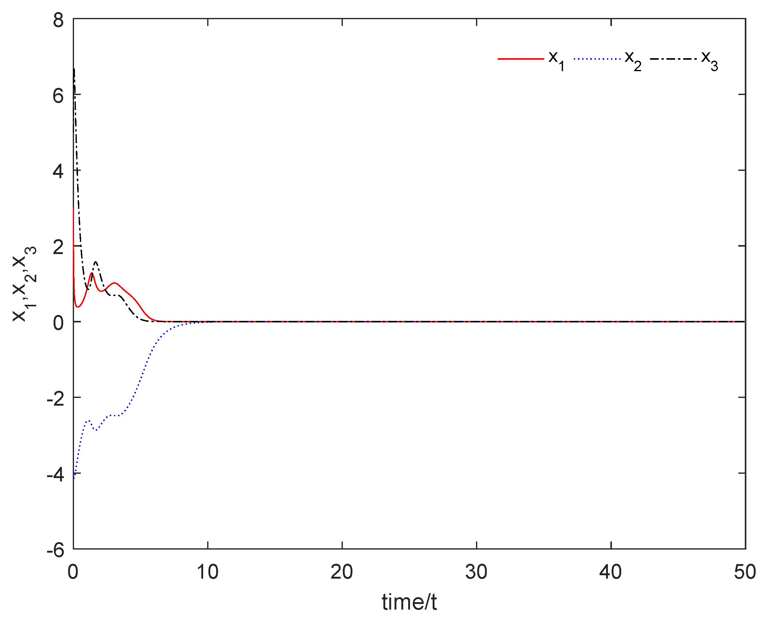
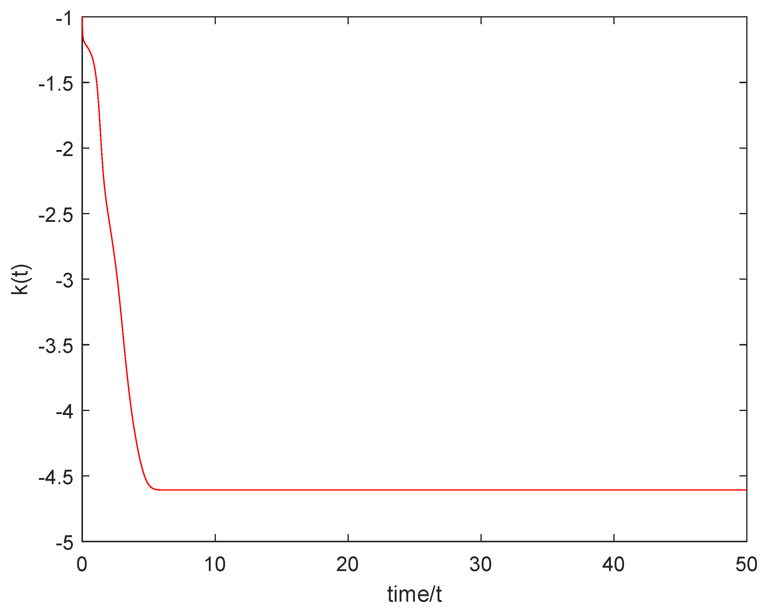
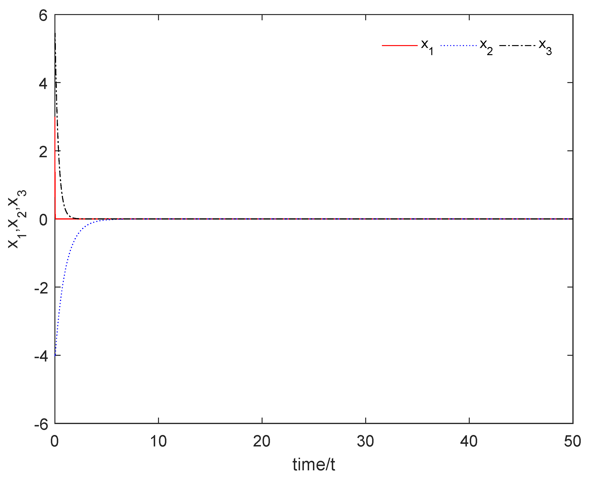
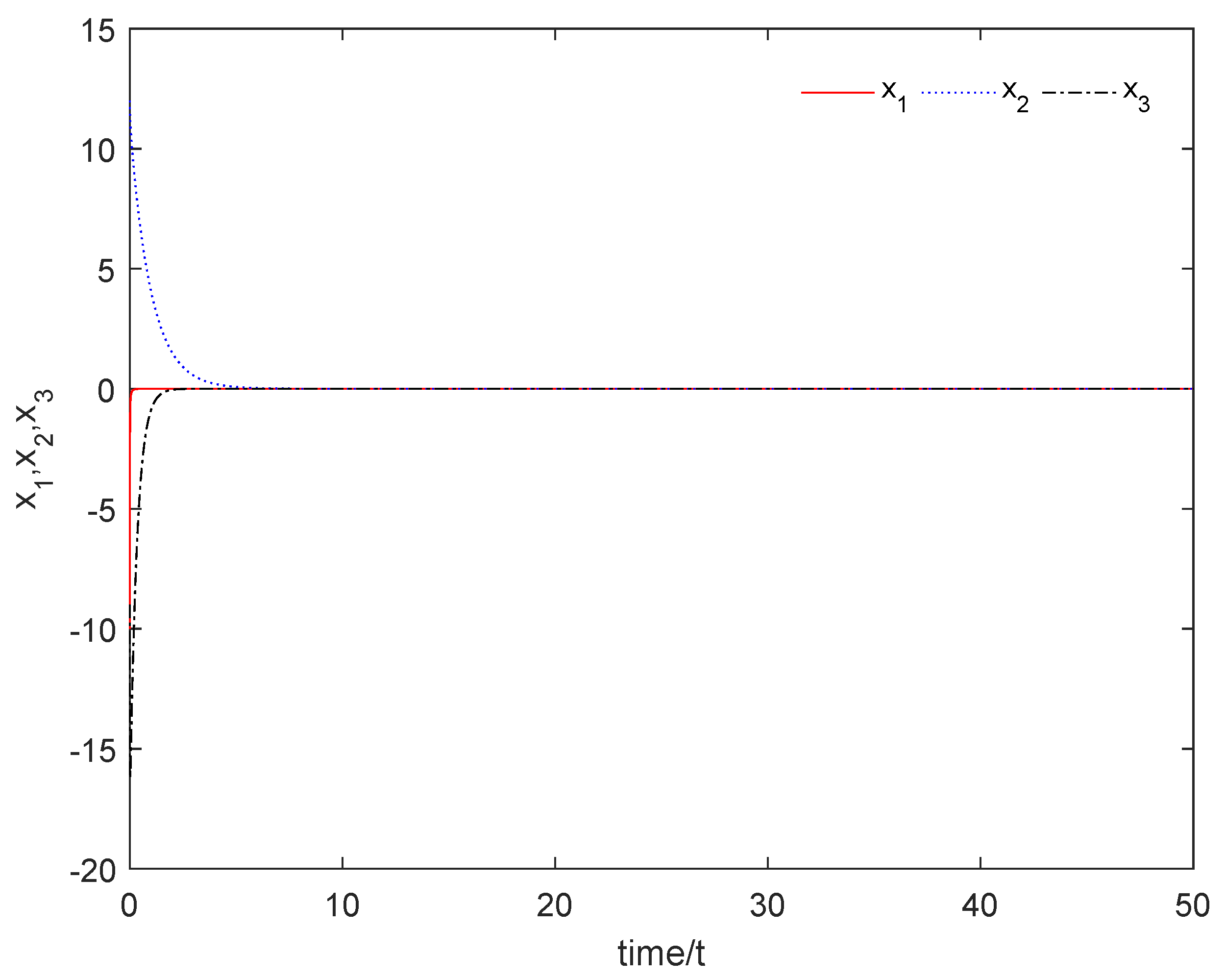
4. The Numerical Simulation

Case 1: The stabilization of the controlled nominal GLV system (4) with the controller $U_c$ is given in (7).

Select the following initial conditions: $x_{c1}\left(0\right)=3$, $x_{c2}\left(0\right)=-4$, $x_{c3}\left(0\right)=5$, and $k\left(0\right)=-1$. Figure 1 shows the controlled nominal GLV system (4) asymptotically stable with respect to the origin. Figure 2 shows that the dynamic feedback gain $k\left(t\right)$ asymptotically tends to a suitable constant.

Case 2: The stabilization of the controlled nominal GLV system (4) with the controller $U_c$ is given in (10).

Select the following initial conditions: $x_{c1}\left(0\right)=3$, $x_{c2}\left(0\right)=-4$, and $x_{c3}\left(0\right)=5$. Figure 3 shows that the controlled nominal system (4) is asymptotically stable with respect to the origin.

Case 3: The stabilization of the controlled GLV system (1) with the controller $U_c$ is given in (7); the external disturbance is $D\left(t\right)=(3t^2+2t+1)e^{0.1t}$, and the DE-based controller $U_D$ is given in (33).

Select the following initial conditions: $x_{c1}\left(0\right)=-10$, $x_{c2}\left(0\right)=12$, $x_{c3}\left(0\right)=-9$, and $k\left(0\right)=-1$. Figure 4 shows that the controlled nominal system (1) is asymptotically stable with respect to the origin. Figure 5 shows that the dynamic feedback gain $k\left(t\right)$ asymptotically tends to a suitable constant. Figure 6 shows that the disturbance estimator $\widehat{D}\left(t\right)$ asymptotically tends to the disturbance $D\left(t\right)$.

5. Conclusions

This paper investigated the stabilization problem of a GLV system with asymptotically unbounded external disturbances and presented some new results. Firstly, two stabilizers were proposed and used to stabilize the nominal GLV system. Then, some appropriate filters were designed and applied to asymptotically track the corresponding disturbances. Based on these filters, two DE-based controllers were designed to realize the stabilization problem. It has been noted that dealing with asymptotically unbounded external disturbances is the biggest advantage of this paper compared to existing results. Finally, the correctness and effectiveness of the proposed results were verified by a numerical simulation.

References

1. Lorenz, E.N. Deterministic non-periodic flow. J. Atmos. Sci. 1963, 20, 130–141. [Google Scholar] [CrossRef]
2. Ott, E.; Grebogi, C.; Yorke, J.A. Controlling chaos. Phys. Rev. Lett. 1990, 64, 1196–1199. [Google Scholar] [CrossRef] [PubMed]
3. Gang, H.; Kaifen, H. Controlling chaos in systems described by partial differential equations. Phys. Rev. Lett. 1993, 71, 3794. [Google Scholar] [CrossRef] [PubMed]
4. Kocarev, L.; Parlitz, U. General approach for chaotic synchronization with applications to communication. Phys. Rev. Lett. 1995, 74, 5028. [Google Scholar] [CrossRef]
5. Guo, R. A simple adaptive controller for chaos and hyperchaos synchronization. Phys. Lett. A 2008, 372, 5593–5597. [Google Scholar] [CrossRef]
6. Zhang, R.; Yang, S. Adaptive synchronization of fractional-order chaotic systems via a single driving variable. Nonlinear Dyn. 2011, 66, 831–837. [Google Scholar] [CrossRef]
7. Yin, C.; Dadras, S.; Zhong, S.M.; Chen, Y. Control of a novel class of fractional-order chaotic systems via adaptive sliding mode control approach. Appl. Math. Model. 2013, 37, 2469–2483. [Google Scholar] [CrossRef]
8. Liang, W.; Lv, X. Li-Yorke chaos in a class of controlled delay difference equations. Chaos Solitons Fractals 2022, 157, 11942. [Google Scholar] [CrossRef]
9. Asiain, E.; Garrido, R. Anti-Chaos control of a servo system using nonlinear model reference adaptive control. Chaos Solitons Fractals 2021, 143, 110581. [Google Scholar] [CrossRef]
10. Long, L.; Zhao, J. Adaptive disturbance rejection for strict-feedback switched nonlinear systems using multiple Lyapunov functions. Int. J. Robust Nonlinear Control 2014, 24, 1887–1902. [Google Scholar] [CrossRef]
11. Hu, J.; Chen, S.; Chen, L. Adaptive control for anti-synchronization of Chua’s chaotic system. Phys. Lett. 2005, 339, 455–460. [Google Scholar] [CrossRef]
12. Ren, B.; Zhong, Q.; Chen, J. Robust control for a lass of non-affine nonlinear systems based on the uncertainty and disturbance estimator. IEEE Trans. Ind. Electron. 2015, 62, 5881–5888. [Google Scholar] [CrossRef]
13. Kuperman, A.; Zhong, Q. UDE-based linear robust control for a class of nonlinear systems with application to wing rock motion stabilization. Nonlinear Dyn. 2015, 81, 789–799. [Google Scholar] [CrossRef]
14. Wang, Y.; Ren, B. Fault ride-through enhancement for grid-tied PV systems with robust control. IEEE Trans. Ind. Electron. 2018, 65, 2302–2312. [Google Scholar] [CrossRef]
15. Li, Y.P.; Guo, R.W.; Liu, L.X. Projective synchronization of the generalized Lotka–Volterra system with asymptotically unbounded external disturbance. Phys. Scr. 2023, 98, 075221. [Google Scholar] [CrossRef]
16. Han, Y.; Ding, J.; Du, L.; Lei, Y. Control and anti-control of chaos based on the moving largest Lyapunov exponent using reinforcement learning. Physica D 2021, 428, 133068. [Google Scholar] [CrossRef]
17. Ding, J.; Lei, Y. Anti-Chaos control of a servo system using nonlinear model reference adaptive control. Physica D 2023, 451, 133767. [Google Scholar] [CrossRef]
18. Cheng, H.; Li, H.; Dai, Q.; Yang, J. A deep reinforcement learning method to control chaos synchronization between two identical chaotic systems. Chaos Solitons Fractals 2023, 174, 113809. [Google Scholar] [CrossRef]
19. Samardzija, N.; Greller, L.D. Explosive route to chaos through a fractal torus in a generalized Lotka–Volterra model. Bull. Math. Biol. 1988, 50, 465–491. [Google Scholar] [CrossRef]
20. Kouichi, M. A concrete example with multiple limit cycles for three dimensional Lotka–Volterra systems. J. Math. Anal. Appl. 2018, 457, 1–9. [Google Scholar]
21. Pastor, J.M.; Stucchi, L.; Galeano, J. Study of a factored general logistic model of population dynamics with inter-and intraspecific interactions. Ecol. Model. 2021, 444, 109475. [Google Scholar] [CrossRef]
22. Long, T.; Liu, C.; Wang, S. The period function of quadratic generalized Lotka–Volterra systems without complex invariant. J. Differ. Equations 2022, 314, 491–517. [Google Scholar] [CrossRef]
23. Manisha, K.; Chrali, B.; Veeresha, P. A chaos control strategy for the fractional 3D Lotka–Volterra like attractor. Math. Comput. Simul. 2023, 211, 1–22. [Google Scholar]
24. Platonov, A.V. Analysis of the dynamical behavior of solutions for a class of hybrid generalized Lotka–Volterra models. Commun. Nonlinear Sci. And Numerical Simul. 2023, 119, 10768. [Google Scholar] [CrossRef]
Figure 1. The controlled nominal GLV system (4) asymptotically stable with respect to the origin.
Mathematics 11 04496 g001
Figure 2. The feedback gain k ( t ) tends to a suitable constant.
Mathematics 11 04496 g002
Figure 3. The controlled nominal GLV system (4) asymptotically stable with respect to the origin.
Mathematics 11 04496 g003
Figure 4. The controlled GLV system (1) asymptotically stable with respect to the origin.
Mathematics 11 04496 g004
Figure 5. The feedback gain k ( t ) tends to a suitable constant.
Mathematics 11 04496 g005
Figure 6. The disturbance estimator D ^ ( t ) asymptotically tends to the disturbance D ( t ) .
Mathematics 11 04496 g006
Disclaimer/Publisher’s Note: The statements, opinions and data contained in all publications are solely those of the individual author(s) and contributor(s) and not of MDPI and/or the editor(s). MDPI and/or the editor(s) disclaim responsibility for any injury to people or property resulting from any ideas, methods, instructions or products referred to in the content.