Abstract
Delta parallel robots have been widely used in precision processing, handling, sorting, and the assembly of parts, and their high efficiency and motion stability are important indexes of their performance.Corners created by small line segments in trajectory planning cause abrupt changes in a tangential discontinuous trajectory, and the vibration and shock caused by such changes seriously affect the robot’s high-speed and high-precision performance. In this study, a trajectory-planning method combining Cartesian space and joint space is proposed. Firstly, the vector method and microelement integration method were used to establish the complete kinematic and dynamic equations of a delta parallel robot, and an inverse kinematic/dynamic model-solving program was written based on the MATLAB software R2020a. Secondly, the end-effector trajectory of the delta parallel robot was planned in Cartesian space, and the data points and inverse control points of the end effector’s trajectory were obtained using the normalization method. Finally, the data points and control points were mapped to the joint space through the inverse kinematic equation, and the fifth-order B-spline curve was adopted for quadratic trajectory planning, which allowed the high-order continuous smoothing of the trajectory planning to be realized. The simulated and experimental results showed that the trajectory-smoothing performance in continuous high-order curvature changes could be improved with the proposed method. The peak trajectory tracking error was reduced by , , and , respectively, and the peak torque change of the three joints was reduced by , , and , respectively.
Keywords:
delta parallel robot; kinematic and dynamic modelling; trajectory smoothing planning; combining Cartesian space with joint space MSC:
34M25
1. Introduction
The delta parallel robot has been widely used in precision parts processing, hanling, sorting, and assembly because of its high speed and high precision [1]. When a straight line or an arc approaches a target curve, the acceleration of the trajectory of the end effector is abrupt due to tangential discontinuity at the connecting corner of the fitted line segment, which makes the vibration of the delta parallel robot inevitable during high-speed operation and even causes production safety accidents [2]. Polynomial functions and interpolation methods are often used for robot trajectory planning and optimization by giving constraints on the starting and ending points, as well as constraints on the displacement, velocity, and acceleration. Boryga [3] presented a smooth trajectory planning method using higher-degree polynomial functions of acceleration to determine accurate dependencies derived for the calculation of polynomial coefficients and motion time in the case of velocity, acceleration, and jerk constraints, thus ensuring the continuity and smoothness of the trajectory. A seventh-order polynomial was applied to the trajectory planning to achieve the position, velocity, acceleration, and jerk of the actuating joints, and the positions/orientations of the parallel mechanism modules were interpolated to obtain a smooth trajectory without impact [4]. To achieve a smooth and precise trajectory while minimizing the jerk, Damasevicius et al. [5] proposed natural cubic splines for finding a Pareto-optimal set of robot arm trajectories. When a robot is required to machine a complex curved workpiece with high precision and speed, the path is generally dispersed into a series of points and transmitted to the robot, which not only reduces the precision, but also causes damage to the motors and robot. To improve the dynamic performance of the delta parallel pickup robot in high-speed pick-and-place processes, taking time and acceleration as optimization objectives, a trajectory optimization method based on the improved butterfly optimization algorithm (IBOA) was proposed [6]. Zhang et al. [7] inserted a quintic Bezier curve between small adjacent line segments to achieve velocity and acceleration continuity at the connecting points, and a quartic polynomial was adopted to achieve a constant velocity at the velocity limitation. To solve the problem of trajectory continuity, some fitting curves were presented, such as quintic and cubic nonuniform rational NURBS curves [8,9], the quintic Pythagorean hodograph (PH) curve [10], combining cubic splines with a linear segment with parabolic blends [11], and the S-curve [12]. However, since the trajectory of the end effector in Cartesian space needs to be mapped to the joint space through the inverse kinematic equation, it is realized by the joint actuator through the torque control according to the calculated joint variable values. Therefore, the end-effector position, joint variables, and the precise modeling of the robot kinematics and dynamics equations impact trajectory smoothing planning and become a very challenging subject in robotics [13,14].
Should surfaces such as sharp corners, holes, or protrusions be considered in trajectory planning [15]? Considering the execution characteristics of joint actuators, most trajectory smoothing planning considers the planning method in joint space. This takes joint velocity, acceleration, and jerk continuity as the trajectory smoothing targets [16,17]. Considering the Gaussian interpolation of the boundary conditions, a radial basis function method was proposed by Chettibi [18] to generate point-to-point smooth trajectories of robot arms. A multiaxis real-time synchronous look-ahead trajectory planning algorithm was proposed by Liang et al. [19] based on dynamically given position and velocity sequences under the constraint of maximum velocity and the acceleration of each joint axis. Shrivastava et al. [20] used the cuckoo search algorithm to suppress the linear motion equation to avoid the directional singularity in Cartesian space. Then, the Bezier curve was used to depict the shape of the joint trajectory by interpolating the linear polynomials with the parabolic blend. In the joint space, the joint movement was divided into acceleration, uniform speed, and deceleration parts; the fourth-order polynomial formed by the root weight was used to plan the acceleration to ensure the continuity of the displacement, speed, acceleration, and jerk of each joint and end effector of the robot [21].
On the other hand, some of the literature has studied the trajectory planning of robot end effectors in Cartesian space [22,23,24,25,26,27]. However, trajectory smoothing planning in a single space cannot guarantee trajectory smoothness in other spaces. Moreover, in the process of high-speed reciprocating motion of a high-speed parallel robot, the influence of its nonlinear dynamic characteristics on the dynamic response and stable operation of the system cannot be ignored, especially when the smooth trajectory is mapped from Cartesian space (or joint space) to joint space (or Cartesian space) [28]. The comprehensive kinematics and dynamics characteristics of the three DoF parallel manipulator were analyzed under the accepted Jacobian link matrices and proverbial virtual work principle, and the discretized piecewise quintic polynomials were employed in order to interpolate the angular positions of the sequence of joints; these were transformed from predefined via points in Cartesian space [29]. Dupac [30] proposed quintic Hermite piecewise interpolants having functional continuity, and the smoothness of the end effector path was guaranteed. At the same time, inverse kinematics and inverse dynamics were used to compute the coordinates of the joints. The smoothness of the trajectory of the robot’s end effector was not only smoothly planned in the Cartesian space, but the kinematic and dynamic changes in the robot joints and the torque generated by the joint actuators were also obtained [31]. This study places a focus on the shock and vibration caused by abrupt trajectory changes, and trajectory-smoothing planning by combining Cartesian and joint space was proposed. The main contributions of this study are summarized in the following:
(1) The delta parallel robot’s complete kinematics/dynamics model was established using vector decomposition and the elementary kinematic energy method. The inverse kinematics/dynamics model of the delta parallel robot was solved using the pseudoinverse matrix solution method, and the mapping relationship between Cartesian space and joint space was constructed.
(2) The trajectory in Cartesian space (end effector) was planned using the normalization method, and data points and inverse points were used to control the mapping accuracy from Cartesian space to joint space.
(3) Using a quintic B-spline curve, combined with the data points and inverse control points, the trajectory planning in the joint space was smoothed.
The rest of this paper is structured as follows: In Section 2, the kinematic and dynamic model of the Delta parallel robot is presented. The trajectory smoothing planning combining Cartesian and joint space is proposed in Section 3. The experimental results are shown in Section 4. Finally, conclusions are drawn in Section 5.
2. Kinematic and Dynamic Model of the Delta Parallel Robot
2.1. Kinematic Model of the Delta Parallel Robot
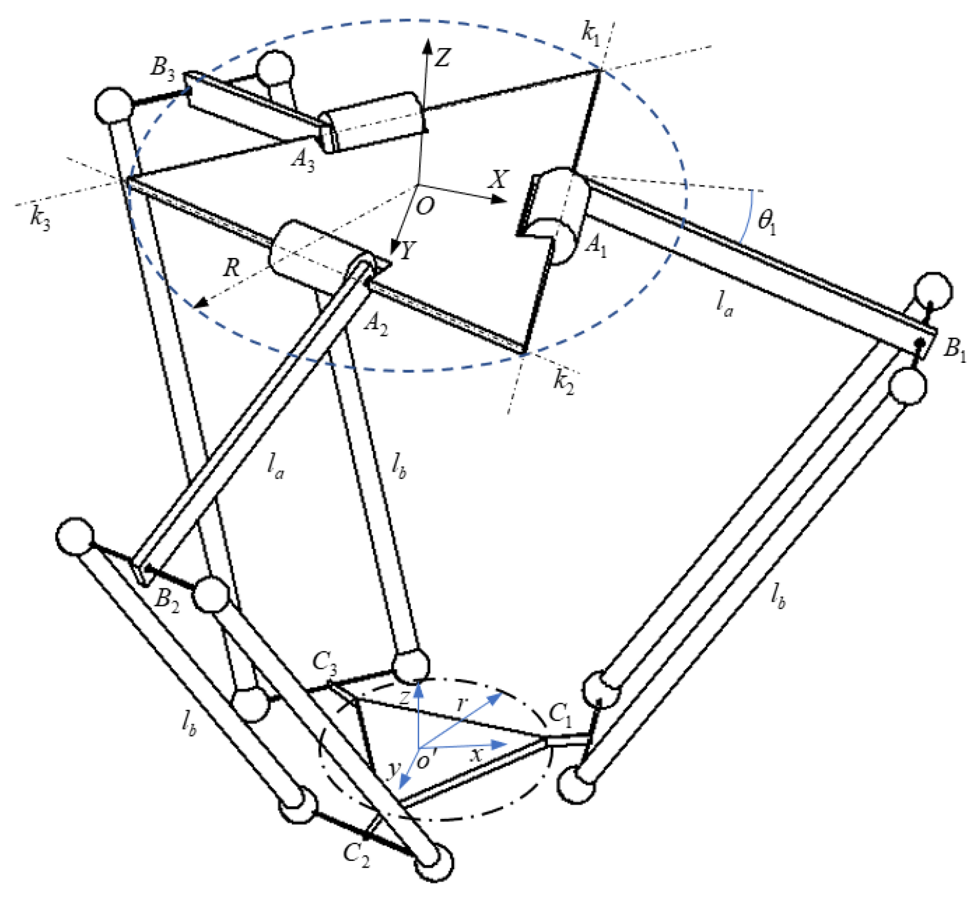
The origin O of the fixed coordinate system is located in the geometric center of the equilateral triangle. The center point () of the three sides of the equilateral triangle is connected to the active link and the fixed platform by revolute joints. The outer tangent circle radius of the equilateral triangle is R, the axis of X is along the direction of , and the axis of Y is parallel to the axis of the revolute joint . The origin of the moving coordinate system is located in the geometric center of the equilateral triangle. The center point () of the three sides of the equilateral triangle is connected to the passive link and the moving platform through a fixed connection. The outer tangent circle radius of the equilateral triangle is r. The length of the active links and passive links are the constant values and , respectively. The variable parameters in joint space are , , and the three output displacements in the Cartesian space of the moving platform are x, y, and z. The geometric configuration of the delta parallel robot is shown in Figure 1.
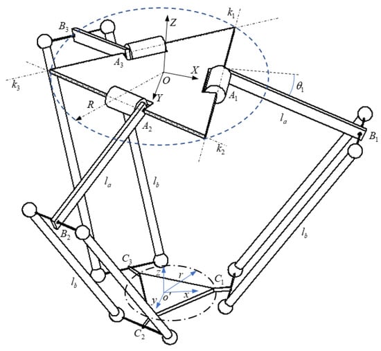
Figure 1.
The geometric configuration of delta parallel robot with three DoFs.
Assume that the origin of the moving platform is with respect to the fixed coordinate system. The inverse positional kinematic of the delta parallel robot can be given by
The axis vectors of the revolute joint are . According to the geometric composition characteristics of the Delta parallel robot, can be derived as follows:
The homogeneous transformation matrix of rotation about any axis is satisfied with
is the changed position of point B in the coordinate system, which can be obtained by translation and rotation based on the initial position , which yields to
is the changed position of point C in the coordinate system, which can be obtained according to the motion characteristics of the moving platform, which yields to
By substituting (4) and (5) into (1), we obtain
where and are the angles between the and X axis, respectively, where .
Assume that and .
Assume that and take the derivative of both sides with respect to the time; thus, we obtain
where is a diagonal matrix, , and , is the velocity vector of the end effector of the delta parallel robot, is the velocity vector of the joints, and is the zero matrix.
Equation (8) can then be rewritten with
where J is the kinematic Jacobian matrix of the delta parallel robot.
By taking the derivative of (9) with respect to the time, we obtain
where and , are satisfied with
and
2.2. Dynamic Model of the Delta Parallel Robot
The dynamic model of the delta parallel robot with three DoFs is given by
where is the inertial mass matrix, is the Coriolis and centripetal force, is the moment, is the gravity matrix. The dynamic equation of the delta parallel robot has the following properties:
Remark 1.
The inertial mass matrix is a positive symmetric matrix and is bounded; it is satisfied by
where m and are constants that are more than zero, and is the identity matrix.
The mass of the active link is , the mass of the passive link is , and the mass of the moving platform is . The mass matrix of the delta parallel robot consists of three parts: an active link , a passive link and a moving platform .
Considering the motion characteristics of the Delta parallel robot, the mass matrix of the moving platform can be expressed as
where is the mass of the moving platform and load, and J is the Jacobian matrix.
The mass matrix of the active link is given by
where , is the moment of inertia of the actuator, and is the mass of the spherical hinge. The linear velocity at any point along the link can be expressed as
where is the velocity at the connection between the , and , is the velocity at the connection between the and the moving platform. The elementary kinematic energy can be given by
where is the material density of the link, and s is the cross-sectional area.
By integrating (17), we obtain
The Jacobian matrix of the joint is defined as , and can be derived as
Assuming that the equivalent mass of the moving platform is , we have the following matrix:
The mass matrix of the delta parallel robot can be expressed completely as
where , and .
3. Trajectory Smoothing Planing Combining Cartesian and Jiont Space
Trajectory smoothing planning of the delta parallel robot combining Cartesian and joint space is mainly conducted to solve the problem of process vibration caused by acceleration and jerk changes, which are caused by discontinuity at the inflection point of the small line segment.
3.1. Trajectory Planning in Cartesian Space
Assume that the end effector of the delta parallel robot passes through the set point , and the complex trajectory consists of multiple microline segments that are connected. The coordinates of each interpolation point are expressed as
where is a normalized factor, is the initial point position, , , and are increments on the x, y and z, respectively, and they are satisfied with
Assume that the velocity of the line in the middle section is v, and the acceleration of the parabola segment is a; the movement time and distance of the parabola segment are satisfied with
where is the run time of the parabola segment, and is the displacement of the parabola segment.
Considering Equation (24), the time, displacement, and acceleration of the parabola segment after normalization can be expressed as
where and are the displacement and time of two adjacent data points, respectively, which are given by
The normalized factor is given by
where , . is the starting point of the line segment, and is the end point of the line segment.
3.2. Trajectory Planning in Joint Space
By using Equations (7)–(22), the interpolation points obtained from Cartesian space are inversely mapped to joint space and used as the critical points of trajectory planning in joint space for quadratic interpolation using the quintic B-spline curve, which is expressed as
where , is the B-spline curve of , are the control points, and is the B-spline basis function, which can be given by
where , and .
By substituting (29) into (28), we obtain
where
When , the end point of the B-spline curve of the fifth dimension is given by
Given data points in joint space , we inverse calculate the control point . Since the number of the control points is , four initial constraint equations are selected as follows:
By combining (30) and (31), we obtain
The method of the inverse control vertex is used to calculate the B-spline curve, and the B-spline curve of degree k is defined as
where is the control vertex of the curve , and is the weight factor whose number is equal to the number of control vertices.
where u is a set of node vectors, which are satisfied with and .
4. Simulations and Experiments
The parameters of the delta parallel robot are shown in Table 1.

Table 1.
Parameters of the delta parallel robot.
The test time was set to 10 s, and the sampling number was set to 20,001. The traditional PID controller was used to verify the single-space (Cartesian space) trajectory smoothing planning, and the proposed trajectory method was compared. The PID controller parameters were set to , , and .
4.1. Simulations
In accordance with Equations (20)–(22), SolidWorks software was used to establish the fixed platform, motor, active link, positive link, and other part models of the delta parallel robot, and after assembly, Adams software was imported to build a multibody dynamic system. We created the interface file with MATLAB in the Adams/Controls module and called the system model established by the Adams software in the MATLAB programming environment. The specific process is as follows:
(1) Save the 3D solid graphics in the SolidWorks software in the format by reading the assembly file of this format inthe Adams software; the delta parallel robot model is imported into the Adams multibody dynamic simulation environment.
(2) Define the material and quality attributes of each part in the Adams environment and add the influence factors of gravity to improve the multibody dynamic system model of the delta parallel robot in the Adams software, as shown in Figure 2a.
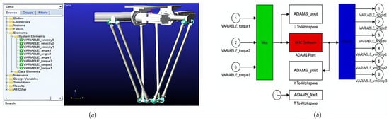
Figure 2.
Simulation platform of the delta parallel robot. (a) The multibody dynamic system model of the delta parallel robot in Adams software. (b) The control block diagram of Adams and MATLAB software united simulation.
(3) Define the system’s state variables (angle/velocity) and create a torque association between the input variables of the system and the single components.
(4) Set up the Adams/Controls module to realize data exchange between the Adams and the MATLAB/Simulink, R2020a and generate the file. The control block diagram of the Adams and MATLAB united simulation is shown in Figure 2b.
Two trajectory comparison methods have been adopted in this paper: one is to map the trajectory planned in Cartesian space to joint space through inverse kinematics (without quadratic trajectory planning), and the other is to map the trajectory planned in Cartesian space to joint space through inverse kinematics and the quintic B-spline curve proposed in Section 2.2 for quadratic trajectory planning.
The end-effector motion trajectory of the delta parallel robot was selected as a five-pointed star curve. A total of 11 data points of the curve were given, and the start and end weight factors were selected as 1.0, respectively; the rest were 0.9. The trajectory of the end effector in Cartesian space is shown in Figure 3.
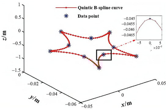
Figure 3.
End-effector trajectory of the delta parallel robot in Cartesian space.
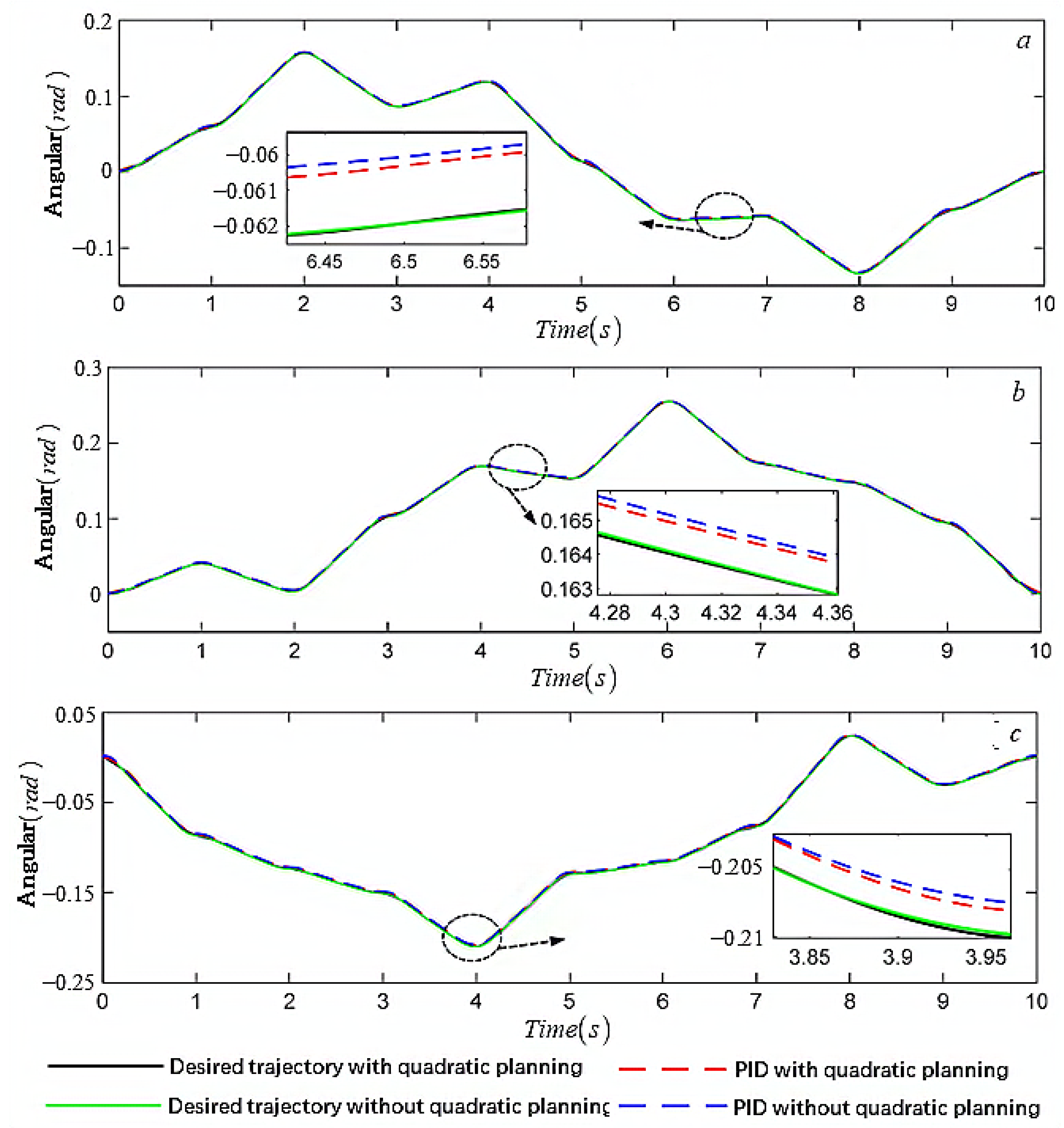
The trajectory planned in the Cartesian space can be mapped to the joint space through the inverse kinematic transformation of the delta parallel robot. If the trajectory of each joint runs according to the mapped trajectory, process vibrations will be generated, which are usually suppressed by the control method. In this paper, the mapped trajectories were quadratically planned so that the trajectories could be smoothed in joint space. When the same PID control was adopted, the trajectory tracking curves of each joint for quadratic planning and nonquadratic planning were derived and are shown in Figure 4. The joint torque is shown in Figure 5. After the process vibrations were suppressed by quadratic trajectory planning, the comparison of quadratic planning trajectory tracking errors as found and is shown in Figure 6.
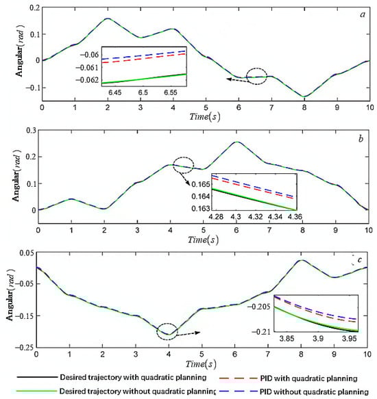
Figure 4.
Trajectory tracking curves of each joint for quadratic planning and nonquadratic planning. (a) Ioint 1. (b) Ioint 2. (c) Ioint 3.
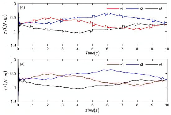
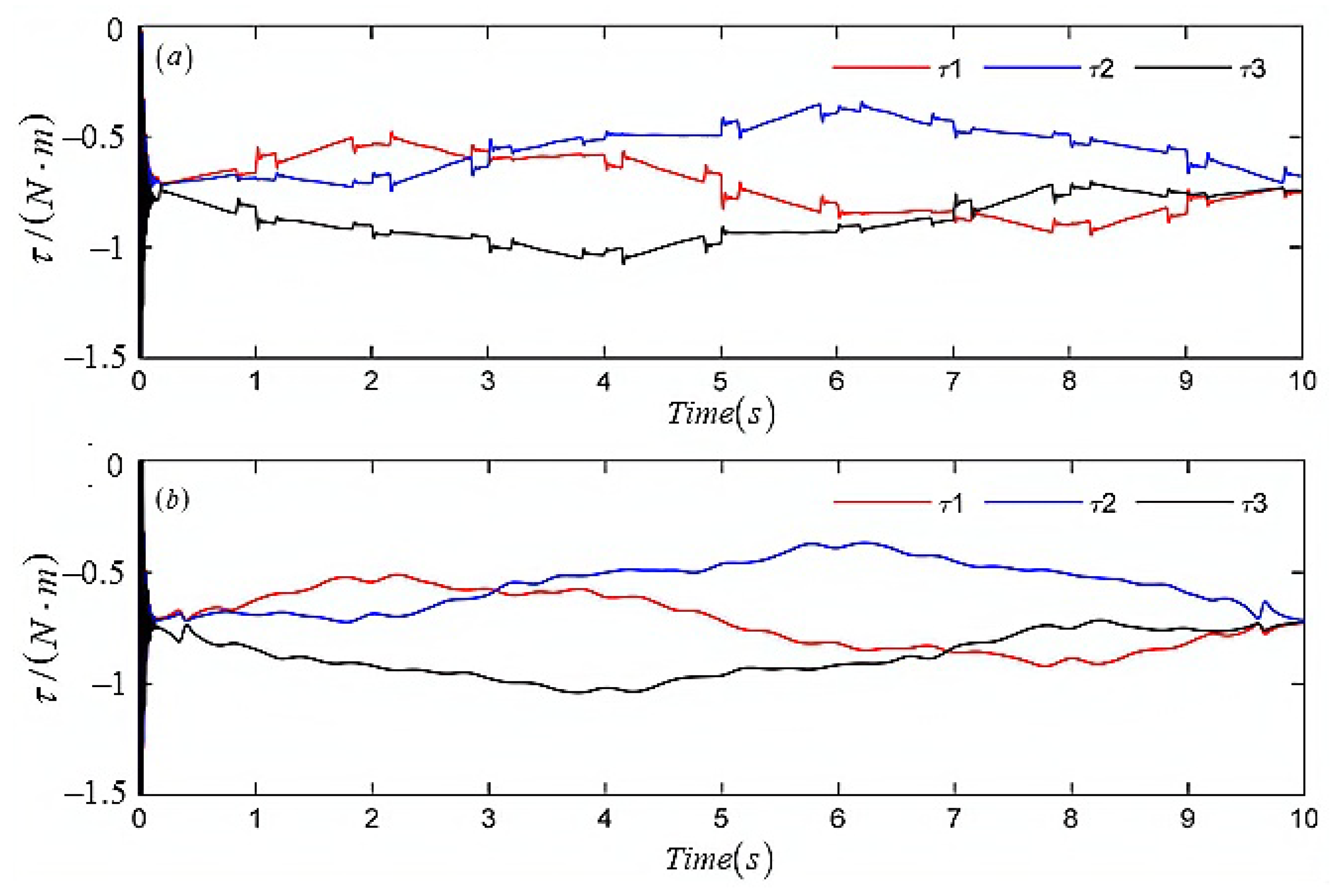
Figure 5.
Joint torque with quadratic planning and nonquadratic planning. (a) Without quadratic planning. (b) With quadratic planning.
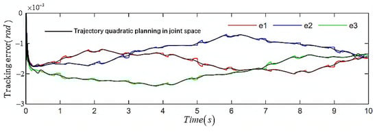
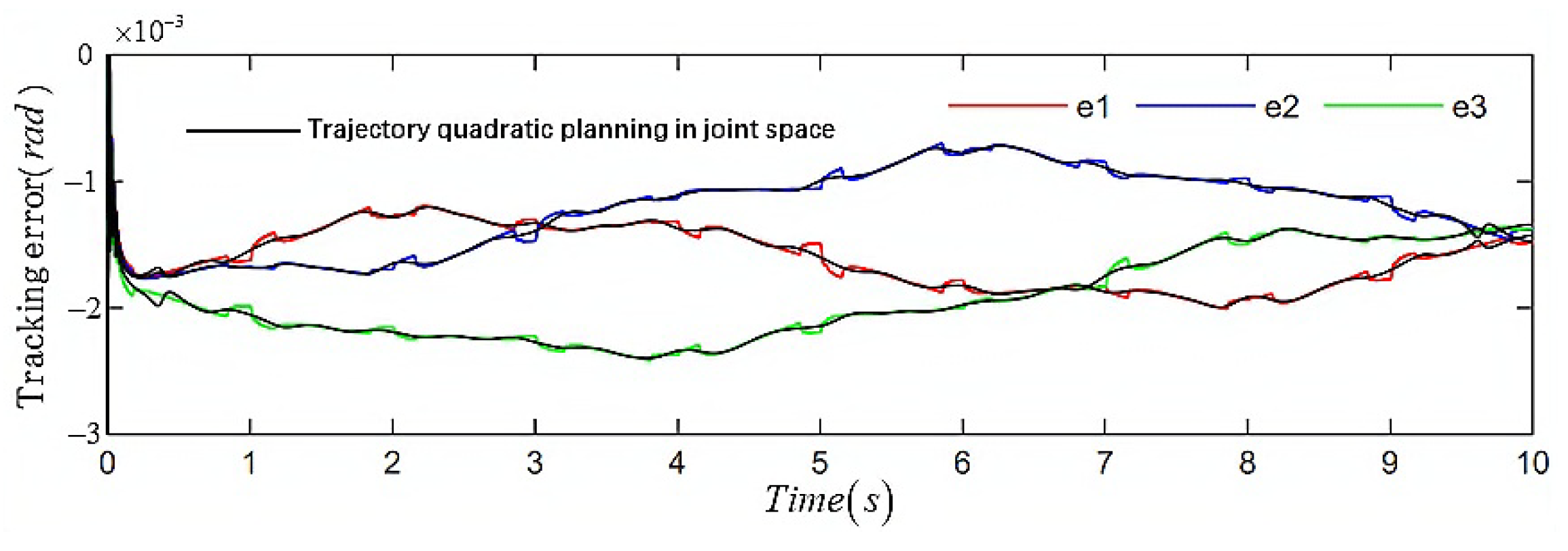
Figure 6.
Trajectory tracking error with quadratic planning in joint space.
Figure 3 and Figure 4 show that the PID controller could effectively track the desired trajectory of the Cartesian space trajectory planning and the quadratic trajectory planning in the joint space, and its steady-state error was kept within . Figure 5 and Figure 6 show that quadratic trajectory planning in joint space could effectively improve the process vibration phenomenon caused by corner discontinuity of the adjacent straight segments. The torque curve was smooth, and the root-mean-square value was reduced. The value pairs of the trace tracking error and control moment root mean square are shown in Table 2.
Table 2.
Comparison of the root mean square of the control moment.
4.2. Experiments
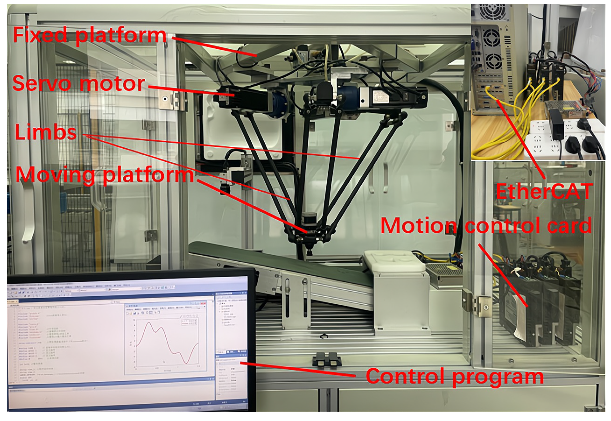
The experimental platform of the delta parallel robot based on the EtherCAT communication mode was constructed. The motion control card was selected from the Googo GEN-009-00 series, which is EtherCAT’s distributed clock device that ensures synchronous movement between the various axes, thus avoiding position deviation in the time response due to the strong coupling characteristics between the various axes. Based on the EtherCAT master–slave architecture, three slave stations were configured on the experimental platform. The model number is JSDG2S-15A-E, and the connection cables are CAT5E-STP RJ45 industrial ethernet cables. The motor model is JSMA-PBC04AAKB, the speed of the motor is 3000 rpm, the rated power is 400 W, the moment of inertia is 0.000073 kg·m, and the reduction ratio of the motor reducer is 1:25. The experimental platform of the delta parallel robot is shown in Figure 7.
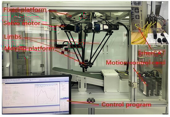
Figure 7.
The experimental platform of the Delta parallel robot.
The interpolation points obtained from Cartesian space were mapped to joint space through inverse kinematics, and the fifth dimension uniform B-spline curve was used as the input data for the second interpolation and trajectory smoothing planning of the angle. The angular velocity, angular acceleration, and angular jerk were obtained in joint space, which are shown in Figure 8, Figure 9 and Figure 10, respectively.
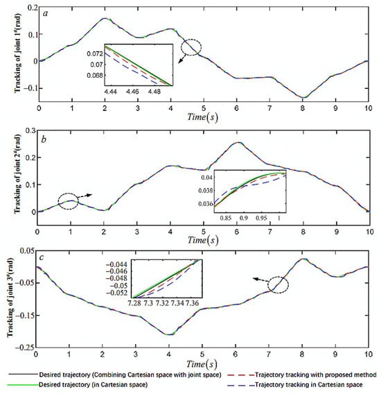
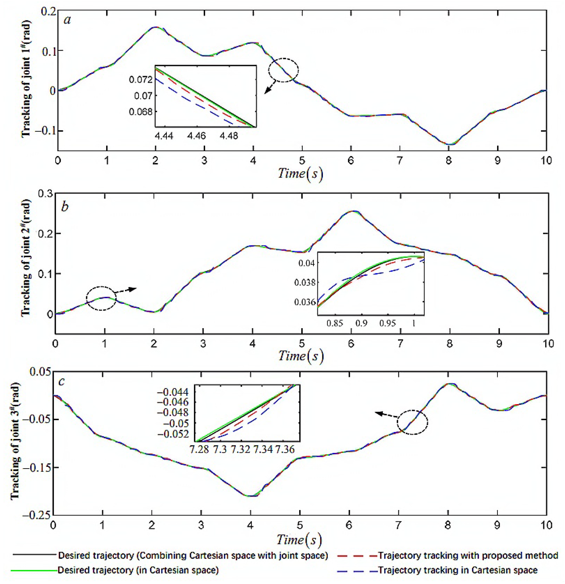
Figure 8.
Trajectory tracking of each joint with proposed method and in Cartesian space. (a) Joint 1. (b) Joint 2. (c) Joint 3.
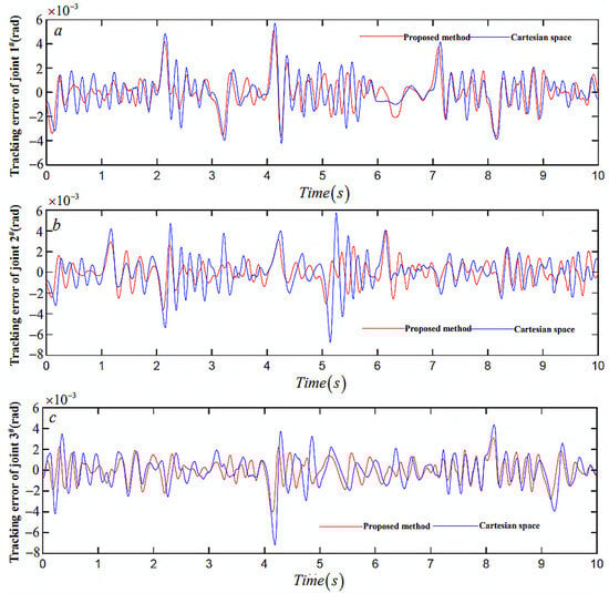
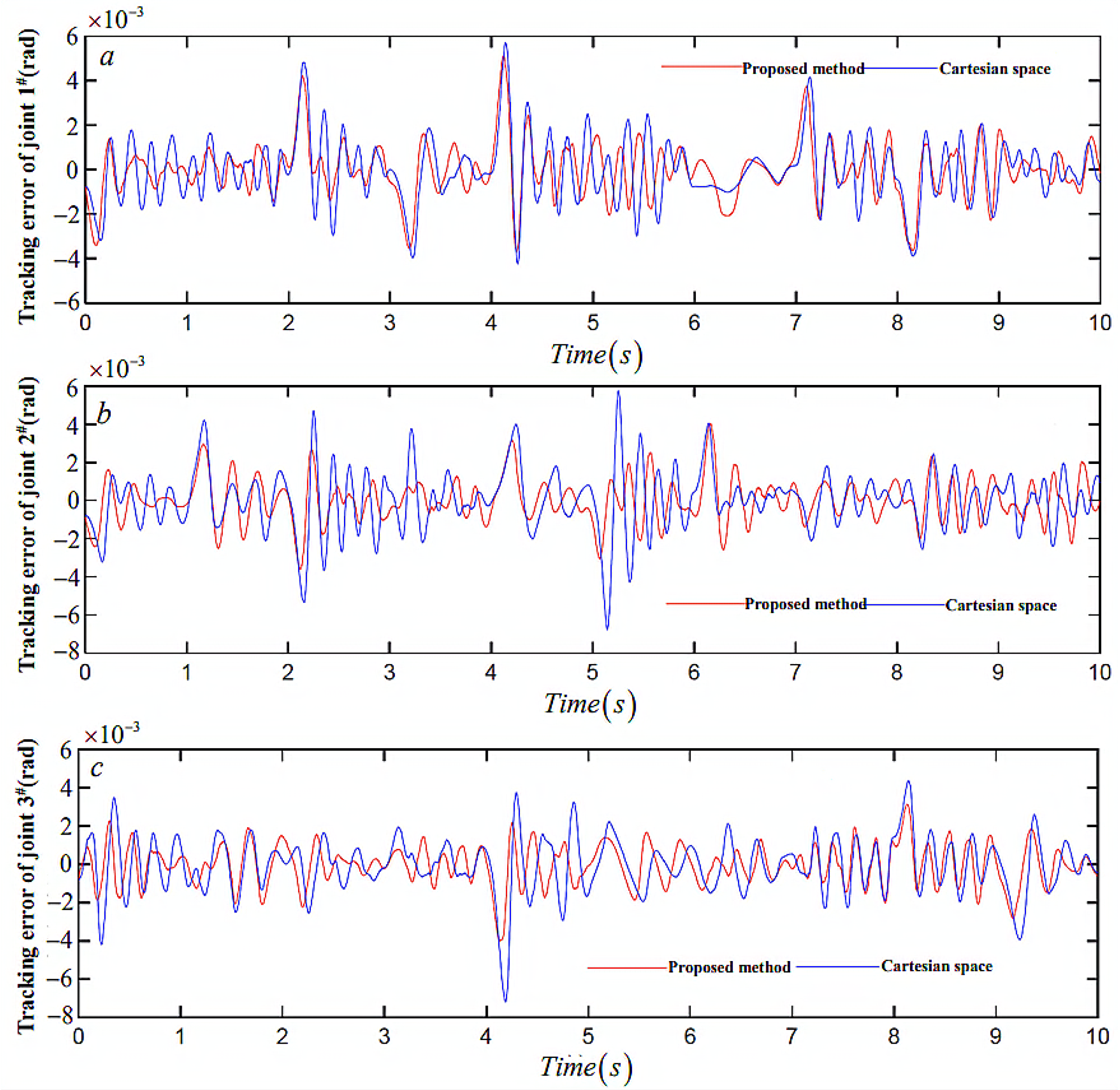
Figure 9.
Tracking error of each joint with proposed method and in Cartesian space. Comparison of joint velocity trajectories in joint space. (a) Joint 1. (b) Joint 2. (c) Joint 3.
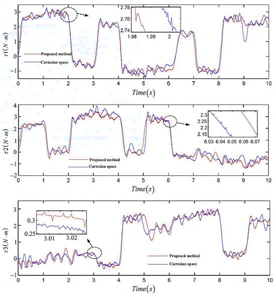
Figure 10.
Comparison of joint acceleration trajectories in joint space.
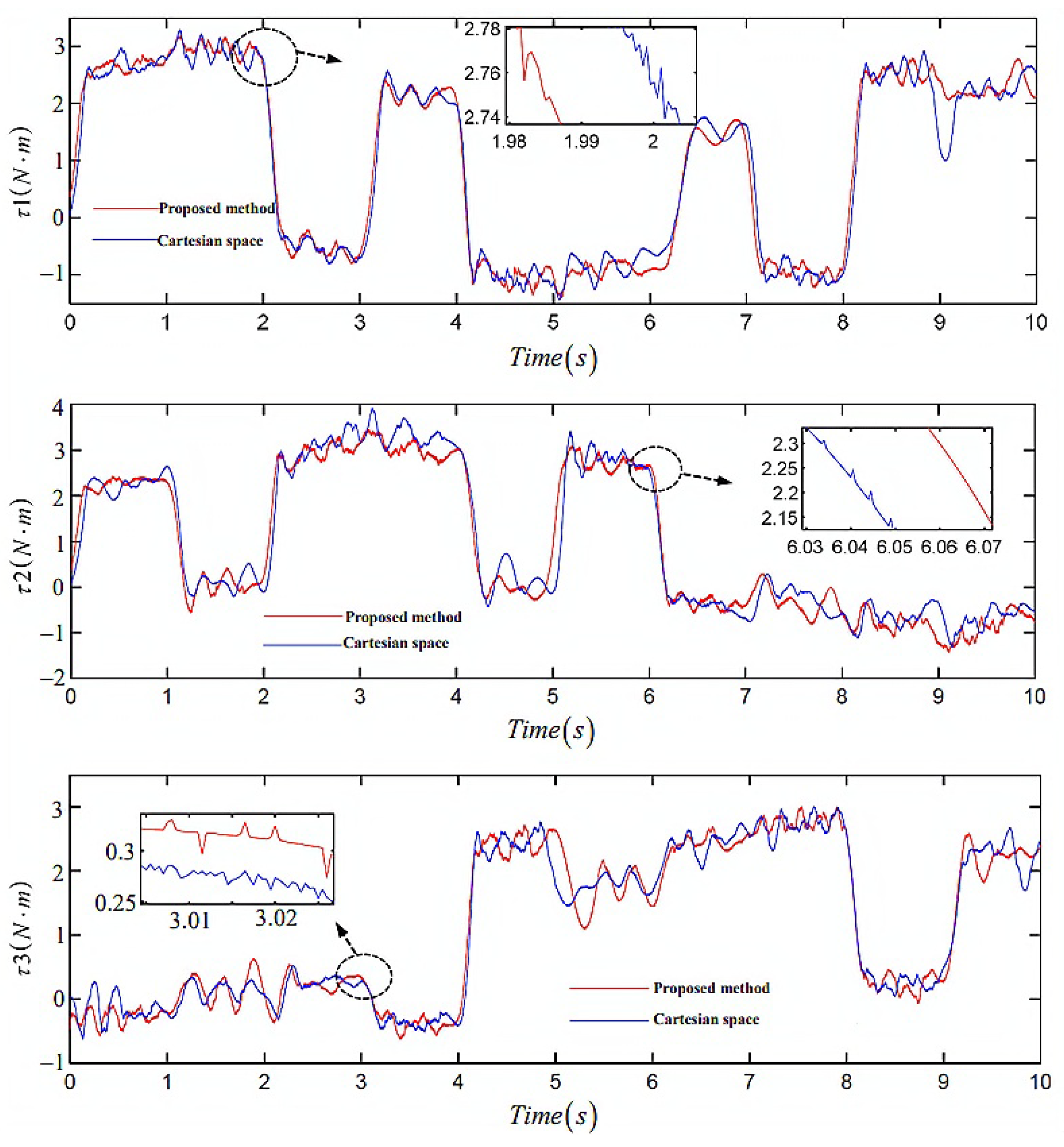
The control torque of the three joints is shown in Figure 10.
Figure 8 and Figure 9 show that, compared to the single-space (Cartesian space) trajectory planning, the trajectory planning algorithm combining joint space could obtain a smoothing trajectory, and the discontinuity of the jerk curve and trajectory mutation could be effectively improved under the same controller (a traditional PID). Among them, the peak tracking errors of joint 2 and 3 were and lower, respectively, than that of the single-space trajectory planning, and the error value of joint 2 was smaller in the 5 s transition stage. The errors rapidly converged at the initial stage of the three joints.
The comparison of the peak values of the trajectory tracking errors is shown in Table 3.
Table 3.
Comparison of the peak values of trajectory tracking errors.
Figure 10 shows that the peak torque reduction rate of joint 2 of the trajectory obtained by the proposed trajectory planning algorithm was , and the torque change trend was gentle. Although the peak torque reduction rates of joints 1 and 3 were and , respectively, it can be seen from the torque amplification diagram that the torque vibration and shock phenomena at the transition of the adjacent line segments, such as 2 s, 3 s, and 6 s, were effectively reduced when the acceleration chattering was improved. A comparison of the peak values of the control torque is shown in Table 4.
Table 4.
Comparison of the peak values of control torque.
5. Conclusions
In order to solve the problem of process shocks and vibrations caused by tangential discontinuity at the corner of small line segments in the trajectory planning of the delta parallel robot end effector, a smooth trajectory planning method based on the combination of the cubic trajectory planning in Cartesian space and the quintic uniform B-spline curve in joint space has been proposed in this paper. (1) The trajectory smoothing planning method combined with Cartesian space and joint space effectively solves the trajectory smoothing problem with the continuous high-order curves’ derivatives, and the obtained joint jerk is continuously smooth. (2) The proposed method can make the robot’s end effector move precisely along a smooth trajectory while making the angular velocity, acceleration, and jerk of the joint continuously smooth without impact. (3) Smooth trajectory planning was carried out from the two aspects of robot kinematics and dynamics, wherein the peak tracking error for joint 1, joint 2, and joint 3 reduced by , and , respectively, and the maximum joint torque reduction was , thereby effectively reducing the vibration and impact during the movement.
Author Contributions
Conceptualization, D.Z. and F.L.; methodology, Y.H.; software, X.Y.; validation, Y.H.; writing—original draft preparation, D.Z.; writing—review and editing, F.L. All authors have read and agreed to the published version of the manuscript.
Funding
This research received no external funding.
Data Availability Statement
The data used to support the findings of this study are available from the corresponding author upon request.
Conflicts of Interest
The authors declare no conflict of interest.
References
- Simionescu, I.; Ciupitu, L.; Ionita, L.C. Static balancing with elastic systems of DELTA parallel robots. Mech. Mach. Theory 2015, 87, 150–162. [Google Scholar] [CrossRef]
- Liu, C.; Cao, G.H.; Qu, Y.Y. Safety analysis via forward kinematics of delta parallel robot using maching learning. Saf. Sci. 2019, 117, 243–249. [Google Scholar] [CrossRef]
- Boryga, M. The use of higher-degree polynomials for trajectory planning with jerk, acceleration and velocity constraints. Int. J. Comput. Appl. Technol. 2020, 63, 337–347. [Google Scholar] [CrossRef]
- Zhao, Y.J.; Yuan, F.F.; Chen, C.W.; Jin, L.; Li, J.Y.; Zhang, X.W.; Lu, X.J. Inverse kinematics and trajectory planning for a hyper-redundant bionic trunklink robot. Int. J. Robot. Autom. 2020, 35, 229–241. [Google Scholar]
- Damasevicius, R.; Maskeliunas, R.; Narvydas, G.; Narbutaite, R.; Polap, D.; Wozniak, W. Intelligent automation of dental material analysis using robotic arm with Jerk optimized trajectory. J. Ambient Intell. Hum. Comput. 2020, 11, 6223–6234. [Google Scholar] [CrossRef]
- Wu, P.; Wang, Z.Y.; Jing, H.X.; Zhao, P.F. Optimal time-jerk trajectory planning for Delta parallel robot based on improved butterfly optimization algorithm. Appl. Sci. 2022, 12, 8145. [Google Scholar] [CrossRef]
- Zhang, S.; Liu, X.J.; Yan, B.K.; Bi, J.; Han, X.D. A real-time look-ahead trajectory planning methodology for multi small line segments path. Chin. J. Mech. Eng. 2023, 36, 59. [Google Scholar] [CrossRef]
- Wu, G.L.; Zhao, W.K.; Zhang, X.P. Optimum time-energy-jerk trajectory planning for serial robotic manipulators by reparameterized quintic NURBS curves. Proc. Inst. Mech. Eng. Part C J. Mech. Eng. Sci. 2021, 235, 4382–4393. [Google Scholar] [CrossRef]
- Xu, G.P.; Zhang, H.; Meng, Z.; Sun, Y.Z. Automatic interpolation algorithm for NURBS trajectory of shoe spraying based on 7-DOF robot. Int. J. Cloth. Sci. Technol. 2021, 34, 434–450. [Google Scholar] [CrossRef]
- Liang, X.; Su, T.T. Quintic Pythagorean-Hodograph curves based trajectory planning for Delta robot with a prescribed geometrical constaint. Appl. Sci. 2019, 9, 4491. [Google Scholar] [CrossRef]
- Bilal, H.; Yin, B.Q.; Kuma, A.; Ali, M.; Zhang, J.; Yao, J.F. Jerk-bounded trajectory planning for rotary flexible joint manipulator: An experimental approach. Soft Comput. 2023, 27, 4029–4039. [Google Scholar] [CrossRef]
- Fang, Y.; Hu, J.; Liu, W.H.; Shao, Q.Q.; Qi, J.; Peng, Y.H. Smooth and time-optimal S-curve trajectory planning for automated robots and machines. Mech. Mach. Theory 2019, 137, 127–153. [Google Scholar] [CrossRef]
- Singh, G.; Banga, V.K. Kinematics and trajectory planning analysis based on hybrid optimization algorithm for an industrial robotic manipulators. Mech. Mach. Theory 2022, 26, 11339–11372. [Google Scholar] [CrossRef]
- Dong, H.; Cong, M.; Chen, H.P. Effective algorithms to find a minimum-time yet high smooth robot joint trajectory. Int. J. Robot. Autom. 2019, 34, 331–343. [Google Scholar] [CrossRef]
- Brown, S.; Pierson, H.A. Adaptive path planning of novel complex parts for industrial spraying operations. Prod. Manuf. Res. 2020, 8, 335–368. [Google Scholar] [CrossRef]
- Wang, F.; Wu, Z.J.; Bao, T.T. Time-jerk optimal trajectory planning of industrial robots based on a hybrid WOA-GA algorithm. Processes 2022, 10, 1014. [Google Scholar] [CrossRef]
- Nadir, B.; Mohammed, O.; Minh-Tuan, N.; Abderrezak, S. Optimal trajectory generation method to find a smooth robot joint trajectory based on multiquadric radial basis functions. Int. J. Adv. Manuf. Technol. 2022, 120, 297–312. [Google Scholar] [CrossRef]
- Chettibi, T. Smooth point-to-point trajectory planning for robot manipulators by using radial basis functions. Robotica 2019, 37, 539–559. [Google Scholar] [CrossRef]
- Liang, Y.Y.; Yao, C.Z.; Wu, W.; Wang, L.; Wang, Q.Y. Design and implementation of multi-axis real-time synchronous look-ahead trajectory planning algorithm. Int. J. Adv. Manuf. Technol. 2022, 119, 4991–5009. [Google Scholar] [CrossRef]
- Shrivastava, A.; Dalla, V.K. Multi-segment trajectory tracking of the redundant space robot for smooth motion planning based on interpolation of linear polynomials with parabolic blend. Proc. Inst. Mech. Eng. Part C J. Mech. Eng. Sci. 2022, 236, 9255–9269. [Google Scholar] [CrossRef]
- Wang, H.; Wang, H.; Huang, J.H.; Zhao, B.; Quan, L. Smooth point-to-point trajectory planning for industrial robots with kinematical constraints based on high-order polynomial curve. Mech. Mach. Theory 2019, 139, 284–293. [Google Scholar] [CrossRef]
- Wang, G.R.; Xu, F.; Zhou, K.; Pang, Z.H. S-velocity profile of industrial robot based on NURBS curve and slerp interpolation. Processes 2022, 10, 2195. [Google Scholar] [CrossRef]
- Grassmann, R.M.; Burgner-Kahrs, J. Quaternion-based smooth trajectory generator for via poses in SE(3) considering kinematic limits in Cartesian space. IEEE Robot. Autom. Lett. 2019, 4, 4192–4199. [Google Scholar] [CrossRef]
- Singh, G.; Banga, V.R. Combinations of novel hybrid optimization algorithms-based trajectory planning analysis for an industrial robotic manipulators. J. Field Robot. 2022, 39, 650–674. [Google Scholar] [CrossRef]
- Zhao, Y.Q.; Mei, J.P.; Niu, M.T. Vibration error-based trajectory planning of a 5-dof hybrid machine tool. Robot. Comput.-Integr. Manuf. 2021, 69, 102095. [Google Scholar] [CrossRef]
- Wang, Q.; Wang, Z.B.; Shuai, M. Trajectory planning for a 6-DoF manipulator used for orthopaedic surgery. Int. J. Intell. Robot. Appl. 2020, 4, 82–94. [Google Scholar] [CrossRef]
- Kelaiaia, R. Improving the pose accuracy of the Delta robot in machining operations. Int. J. Adv. Manuf. Technol. 2017, 91, 2205–2215. [Google Scholar] [CrossRef]
- Yang, D.; Xie, F.G.; Liu, X.J. Velocity constraints based approach for online trajectory planning of high-speed parallel robots. Chin. J. Mech. Eng. 2022, 35, 127. [Google Scholar] [CrossRef]
- Lu, S.; Ding, B.X.; Li, Y.M. Minimum-jerk trajectory planning pertaining to a translational 3-degree-of-freedom parallel manipulator through piecewise quintic polynomials interpolation. Adv. Mech. Eng. 2020, 12, 1687814020913667. [Google Scholar] [CrossRef]
- Dupac, M. Mathematical modeling and simulation of the inverse kinematic of a redundant robotic manipulator using azimuthal angles and spherical polar piecewise interpolation. Math. Comput. Simul. 2023, 209, 282–298. [Google Scholar] [CrossRef]
- Rout, A.; Deepak, B.B.V.L.; Biswal, B.B.; Mahanta, G.B. Trajectory generation of an industrial robot with constrained kinematic and dynamic variations for improving positional accuracy. Int. J. Appl. Metaheuristic Comput. 2021, 12, 163–179. [Google Scholar] [CrossRef]


Disclaimer/Publisher’s Note: The statements, opinions and data contained in all publications are solely those of the individual author(s) and contributor(s) and not of MDPI and/or the editor(s). MDPI and/or the editor(s) disclaim responsibility for any injury to people or property resulting from any ideas, methods, instructions or products referred to in the content. |
© 2023 by the authors. Licensee MDPI, Basel, Switzerland. This article is an open access article distributed under the terms and conditions of the Creative Commons Attribution (CC BY) license (https://creativecommons.org/licenses/by/4.0/).