Abstract
The recycling of waste products can bring enormous economic and environmental benefits to supply chain participants. Under the government’s reward and punishment system, the manufacturing industry is facing unfolded pressure to minimize carbon emissions. However, various factors related to the design of closed-loop logistics networks are uncertain in nature, including demand, facility capacity, transportation cost per unit of product per kilometer, landfill cost, unit carbon penalty cost, and carbon reward amount. As such, this study proposes a new fuzzy programming model for closed-loop supply chain network design which directly relies on fuzzy methods based on the necessity measure. The objective of the proposed optimization model is to minimize the total cost of the network and the sum of carbon rewards and penalties when selecting facility locations and transportation routes between network nodes. Based on the characteristics of the problem, a genetic algorithm based on variant priority encoding is proposed as a solution. This new solution encoding method can make up for the shortcomings of the four traditional encoding methods (i.e., Prüfer number-based encoding, spanning tree-based encoding, forest data structure-based encoding, and priority-based encoding) to speed up the computational time of the solution algorithm. Several alternative solution approaches were considered to evaluate the proposed algorithm including the precision optimization method (CPLEX) and priority-based encoding genetic algorithm. The results of numerous experiments indicated that even for large-scale numerical examples, the proposed algorithm can create optimal and high-quality solutions within acceptable computational time. The applicability of the model was demonstrated through a sensitivity analysis which was conducted by changing the parameters of the model and providing some important management insights. When external parameters change, the solution of the model maintains a certain level of satisfaction conservatism. At the same time, the changes in the penalty cost and reward amount per unit of carbon emissions have a significant impact on the carbon penalty revenue and total cost. The results of this study are expected to provide scientific support to relevant supply chain enterprises and stakeholders.
Keywords:
closed-loop logistics; carbon emissions; government reward and punishment mechanisms; necessity measure; fuzzy programming MSC:
49K10
1. Introduction
The emergence of scrap and returns has further increased the severity of environmental issues [1]. To this end, governments and enterprises around the world have taken numerous measures. At the 2015 United Nations Summit on Sustainable Development, the 2030 Agenda for Sustainable Development was unanimously adopted with systematic planning covering three aspects of sustainable development, namely, social, economic, and environmental. Since the development of logistics, people have no longer limited their vision to the forward flow of products but have started to seek opportunities from reverse recycling logistics. Closed-loop logistics combines forward and reverse logistics activities to form a complete logistics cycle from procurement to final sales and then the return of used products, solving the problem of product recycling [2]. Thus, alternatives for achieving environmentally friendly development of the social economy are receiving increasing attention from the community. As the main body of social and economic development, logistics is crucial for enterprises to mitigate resource waste and achieve a resource-saving development model which is essential for achieving the above goals.
It should be pointed out that logistics activities have a significant impact on the environment throughout the entire lifecycle of a product, with their carbon dioxide emissions accounting for 15% of the total emissions and approximately 7% of all human activity emissions. Moreover, carbon emissions during transportation can account for over 80% of the total logistics emissions [3]. According to the World Economic Forum Supply Chain Low Carbon Report released by Accenture Consulting, if the relevant logistics network structure can be scientifically and reasonably planned, the global annual carbon dioxide emissions can be decreased by more than 1.4 billion tons. Hence, in a green closed-loop supply chain, the core that affects its efficiency is the closed-loop logistics network. In other words, a scientific and reasonable logistics network can effectively reduce supply chain operating costs, improve material or product transportation efficiency, and decrease carbon dioxide emissions in the logistics process. However, the investment and renovation costs of logistics infrastructure are often high and once the relevant facilities are determined, they are difficult to change. To this end, a reasonable site selection plan is the foundation for ensuring the efficiency of the logistics network.
The development of closed-loop logistics over the past decade, especially the widespread attention it has received from countries around the world, cannot be separated from the policy support and legal regulations of governments around the world. Usually, the profits generated by reverse logistics for each member of the supply chain are not enough to motivate all supply chain members to participate in recycling and remanufacturing activities and the profit margin obtained by manufacturers is only 3–5%. In response, the participation of closed-loop logistics members in recycling and remanufacturing requires government incentives and guidance (recycling subsidies, recycling rewards and punishments, etc.). Contemporary environmental problems are becoming more and more serious. Human beings are facing the crisis of environmental pollution and climate change. Governmental agencies propose to vigorously develop low-energy consumption, high-yield industries, and a low-carbon economy. Therefore, governmental agencies impose constraints on carbon emissions during the product manufacturing process (carbon emission quotas, carbon emission reward, and punishment mechanisms) requiring manufacturing enterprises to improve production technology and reduce unit carbon emissions to decrease greenhouse gas emissions [4]. In doing so, based on the current resource and environmental pressure, exploring the government’s incentive mechanism for carbon emissions and recycling and remanufacturing in closed-loop logistics is of considerable contemporary value.
The natural complexity of closed-loop logistics leads to a high degree of uncertainty in its structure with a focus on strategic logistics network structures [5]. The main reasons include the following: (1) market turbulence leading to uncertain demand; (2) the different locations of logistics network nodes result in uncertainty in facility capacity and transportation costs per unit of product per kilometer; (3) uncertainty in the treatment standards for landfill waste in different regions; and (4) the government’s efforts to encourage enterprises to actively reduce carbon emissions have led to uncertainty in the number of rewards and the unit penalty cost. The above uncertainties are necessary considerations, which is another key issue considered in this manuscript.
According to existing research results, common problems in the design of closed-loop logistics networks, such as facility location selection and path optimization, generally belong to the category of NP-hard problems [6,7]. The solving time of such problems generally increases exponentially with the increase in scale and the difficulty of solving in uncertain environments is often greater [8]. So, how to efficiently obtain the optimal solution to related problems is also the key to solving the above problems and ensuring the optimality and feasibility of relevant research methods and solutions. Due to the complexity of the optimization problem itself, seeking efficient and accurate solutions for its related models is another crucial issue. Therefore, it is necessary to study model-solving algorithms for the above problems.
In summary, the main contribution outlooks of this work to the state of the art include the following: (1) establishing a network planning model based on the original general closed-loop model taking into account the location of landfill sites, carbon emission limits, and government rewards and punishments; (2) capturing uncertain parameters that are often ignored in closed-loop logistics network models and describing them using the appropriate model measures to determine the necessary level of uncertain parameters; and (3) building a new variant priority encoding method within a metaheuristic algorithm for closed-loop logistics networks which is easier to implement and understand when comparing to the existing methods. The advanced achievements include the following: (1) assist enterprises in establishing a stable closed-loop logistics network; (2) assist in providing government decision making on carbon emissions; and (3) induce enterprises to change toward green emission reduction.
The structure of this study is as follows: Section 2 presents a literature review on closed-loop supply chain problems and relevant attributes associated with this study. Section 3 provides a mathematical model for the closed-loop supply chain network problem under consideration. Section 4 provides a detailed explanation of the new solution encoding method for genetic algorithms with variant priority encoding. Section 5 conducts a numerical experiment that uses several examples generated from real data ranges at different scales to test the efficiency of the proposed algorithm and carries out a sensitivity analysis on changes in carbon emission limits and government reward and punishment parameters. Finally, management insights are extensively discussed in Section 5 as well. Section 6 presents the conclusions of current research and future research recommendations.
2. Literature Review
Environmental protection issues have become a global hotspot and governments around the world have successively introduced carbon reduction policies and regulations for various industries. The improper management of transportation networks, logistics centers, and transportation and distribution operations induces excessive carbon emissions in the logistics industry [9]. Closed-loop logistics has the function of utilizing resources and reducing pollution. However, the closed-loop logistics network still needs appropriate management in recycling, remanufacturing, transportation, and distribution operations to reduce the carbon emissions generated by energy consumption during logistics operations. As such, an efficient network design is the key to solving the associated decision problems. A substantial number of models have been developed over the years aiming to facilitate the design of closed-loop supply chain networks. This section of the manuscript provides a review of the literature relevant to the theme of the present study.
2.1. Closed-Loop Logistics
Closed-loop logistics networks are based on the production and transportation activities of manufacturing or production enterprises. They are the strategic layout of the transportation process for a certain period. In recent studies, most scholars have focused on the research of closed-loop logistics networks in a particular industry. In agriculture, Salehi-Amiri et al. [10] designed a new closed-loop supply chain network for the walnut industry and established a new mixed integer linear programming which not only meets the needs of various markets but also makes preparations for the secondary use of returned products. Rajabi-Kafshgar et al. [11] considered the environmental impact of agricultural waste and the safety of agricultural products and established a new hybrid linear mathematical model for agricultural supply chain networks to minimize the fixed and variable total costs of closed-loop supply chains. In the e-commerce industry, Prajapati et al. [12] developed a sustainable framework and a mixed integer nonlinear programming model for the multi-level and multi-electronic product closed-loop supply chain in the e-commerce industry to reduce the total costs associated with the forward and reverse flow of goods in the closed-loop supply chain and maximize the revenue.
In terms of economic phenomena, Kim and Chung [13] established a supply chain model to investigate the impact of backflow on strengthening the manufacturing industry and address issues, such as economic recession and job shortages, in order to determine whether manufacturing centers, suppliers, and reverse logistics facilities should be relocated from the host country to their home country, and maximize total profits based on the level of backflow drivers in the traditional manufacturing industry. Lu et al. [14] studied the production and logistics coordination scheduling problem for a large-scale closed-loop manufacturing system, designed a decentralized network, and expressed the coordination scheduling problem as a mixed integer programming model that includes both binary and integer variables. They developed an iterative solution method based on Bender’s decomposition which improves the solution efficiency in large-scale situations by updating custom constraints. Ullah [15] constructed a hybrid manufacturing remanufacturing model under different reverse channel structures and captured the effects of transportation distance and cost on the environmental and economic performance of closed-loop supply chains. Furthermore, the study examined the relationship between the transportation distance and cost, remanufacturing rate, optimal reverse channel, and system net emissions. In terms of energy, Köseli et al. [16] focused on reducing CO2 emissions in refrigerated transportation systems, collecting and treating waste to reduce energy waste, and providing employees with more attractive work schedules to promote sustainable business management. In terms of healthcare, Mondal and Roy [17] established a less infectious network by designing the transportation problem and the pickup truck routing problem into two stages and delivering them separately. The above literature has laid a foundation for optimizing closed-loop logistics networks in sustainability and applications in the energy, healthcare, and agricultural sectors. However, we still need to consider the impact of waste on the environment.
There are different ways to model closed-loop logistics networks for different industries. However, in academic research, it is more important to study general closed-loop logistics networks which can be further extended to different industries and specific applications. The most representative example is Wang and Hsu [18] who proposed a general closed-loop logistics structure with suppliers, factories, distribution centers, customer points, and dismantling centers. Nevertheless, the structure design involves burying non-recyclable waste in the dismantling center without considering the damage to the local environment. To this end, this study adds the location selection of landfill sites and the transportation process from the dismantling center to the landfill site.
2.2. Carbon Emissions
The closed-loop logistics network itself has the environmental protection function of reducing resource waste but it cannot conceal the occurrence of carbon emissions during its operation. Therefore, researchers have started to study the quantification of carbon emissions during logistics activities. Benjaafar et al. [19] took the lead in explaining how to incorporate carbon emissions into operational decisions in procurement, production, and inventory management in supply chain management. The study showed how to modify the traditional model by associating carbon emissions parameters with various decision variables to support decisions that simultaneously consider costs and carbon footprint. Afterward, scholars began to study different carbon-related perspectives. In terms of resource matching, Wang et al. [20] identified the problem of achieving ideal supply and demand matching of logistics resources. Using supply and demand data of logistics service users, they proposed a green city closed-loop logistics distribution network model to obtain an optimized solution that minimizes greenhouse gas emissions and overall operating costs. The results indicated that under the shortest delivery route, there is a negative correlation between cost and carbon emissions.
In terms of price competition and carbon emissions, Wang et al. [21] investigated the design of competitive and sustainable supply chain networks, studied the retail price and carbon emissions equilibrium during the competition stage, and substituted the equilibrium results of the competition stage as constraints into the network design stage. Regarding food supply chains, Purnomo et al. [22] examined the sustainable and traceable closed-loop supply chain network of fish, considered the carbon emissions of transportation, production, and warehouse activities, and used mixed integer linear programming (MILP) to minimize the total cost which includes production and traceability costs, transportation costs, inventory costs, and emission costs. However, the above research models only the proactive carbon emission behavior of enterprises while, in reality, the government has a role in managing and guiding the greening of supply chain activities. Therefore, some scholars began to study the carbon tax and quota policies. For example, Nausheen et al. [23] considered the carbon tax policy and developed a multi-objective closed-loop supply chain model to optimize the distribution plans and minimize transportation and other operating costs and carbon footprint which can help decision-makers to determine the optimal internal carbon price for enterprises. A case study of small leather industry based in India was conducted as a part of the study as well. In addition, Xiao et al. [24] calculated the carbon emissions generated and reduced by public bicycles throughout their entire lifecycle based on lifecycle theory.
Carbon taxes and carbon emission quotas are only one approach of how the government guides enterprises to conduct green operations. The incentives and punishment mechanisms can be adopted from management science. The government can form a certain binding or incentive force on enterprises through the use of reward and punishment mechanisms such as by punishing enterprises producing a large amount of carbon emissions and rewarding them if not. Nevertheless, there is currently little research on this aspect that focuses more on the discussion between the government and enterprises and there is a lack of research on the degree of government rewards and punishments from the perspective of simultaneously optimizing enterprise logistics activities.
2.3. Uncertainty
Uncertainty seriously affects the management of logistics networks. In terms of stochastic programming, Rahimi and Ghezavati [25] identified the network design problem with stochastic demand and the investment rate of recycled products. Considering the uncertainty in the model, two-stage stochastic programming with conditional risk aversion was proposed. Kchaou-Boujelben et al. [26] established two-stage stochastic programming with dual objectives for a closed-loop supply chain to illustrate the difficulties in predicting and controlling recyclable projects in practice. In terms of fuzzy programming, Garai and Sarkar [27] recognized the financial self-sufficiency problem of reverse chain and established a cost-effective and customer-centric closed-loop supply chain model to solve the recycling problem of second-generation biofuels and casing soil. They also proposed the Pareto optimal solutions for the satisfaction of Chinese herbal retail customers and second-generation biofuel major customers in fuzzy situations.
In terms of robust optimization, Kim et al. [28] proposed a closed-loop supply chain robust optimization model to address the uncertainty of recycled products and customer demand in the fashion industry. To avoid the conservatism of robust solutions, they suggested an alternative optimization model that utilizes uncertain budgeting. In terms of combining stochastic programming with robust optimization, Shahparvari et al. [29] established a robust stochastic optimization model for reverse logistics in closed-loop supply chains. By employing chance-constrained robust stochastic programming (CCRSP) to determine the optimal flow of products, the study emphasized how the number of factory openings could be affected by the price change in carbon credit and proposed a hybrid particle swarm optimization algorithm for a practical case study of the automobile manufacturing industry. Eslamipoor [30] considered risk and environmental factors and established a closed-loop supply chain mixed integer programming model using two-stage stochastic programming and scenario-based methods. The model directly captured the uncertainty of customer demand and the impact of customer return rates on the network structure.
The reviewed literature indicates that research on closed-loop logistics often focuses on uncertainty from one or more theories, including stochastic, fuzzy, and robust optimization. Among the three uncertainty modeling methods, the advantage of fuzzy planning consists of fact that the probability distributions are not required for modeling uncertain parameters. The fuzzy set theory can be used to define the uncertain parameter data. Hence, this study will use fuzzy planning to study closed-loop logistics with uncertain parameters.
To address the ambiguity of the objective function and constraint conditions, the opportunity-constrained fuzzy programming method is adopted for transforming certain objective function components and constraint sets that are subject to uncertainty [31,32]. Chance-constrained fuzzy programming methods are divided into the possibility transformation (Pos) and necessity transformation (Nec) methods which are also fully applicable to various forms of fuzzy numbers (such as triangles and trapezoids). The optimality of these two transformations can be defined based on randomness theory as the best solution to possibility and necessity. In other words, the most likely solution means that there is at least one possible optimal solution. On the other hand, the best solution to inevitability means that making all possible solutions solvable is optimal. In doing so, using the necessity transformation is more meaningful in meeting the opportunity constraints than the possibility transformation.
2.4. Solution Algorithms
At present, there are various solution approaches for solving the optimization problems related to closed-loop logistics networks, including heuristic algorithms and metaheuristic algorithms. The recent research is mainly focused on developing new algorithms for closed-loop supply chains. The new algorithms tend to change the individual selection and transformation processes. However, the encoding method of the metaheuristic algorithms can substantially affect the algorithmic performance. For the closed-loop supply chain network design problem, most of the current literature mainly adopts the following solution encoding methods: (1) Prüfer number-based encoding [33], (2) spanning tree-based encoding [34], (3) forest data structure-based encoding [35,36], and (4) priority-based encoding [37,38,39,40,41,42,43,44,45], to name a few. However, the four encoding methods mentioned above are complex and may require repair operations, making the decoding process difficult and increasing the algorithm’s running time. Based on this, this paper proposes a genetic algorithm with a new variant priority encoding scheme (VPGA) and employs this algorithm for the decision problem studied herein.
In summary, this study considers the general closed-loop logistics model consisting of suppliers, factories, distribution centers, customer points, dismantling centers, and landfill sites. Under the constraints of carbon emission quotas, the aim is to construct a generalized strategic planning model for a multi-level closed-loop logistics network to minimize the sum of government reward and punishment costs and the total operating costs of the relevant supply chain. Uncertainty in various factors, such as demand, facility capacity, transportation cost per unit of product per kilometer, landfill cost, unit penalty cost, and reward amount are directly incorporated within the proposed modelling framework. The necessity measure is applied to address the uncertainty of the aforementioned supply chain parameters [31,32]. Last but not least, a genetic algorithm which deploys a variant priority encoding (VPGA) for encoding the candidate solutions is developed as a solution approach.
3. Problem Description and Uncertainty Modeling
3.1. Problem Definition
Logistics is the physical flow process of goods from the point of origin to the point of consumption. To meet user needs, functions, such as transportation, storage, procurement, loading and unloading, packaging, circulation processing, distribution, and information processing, are planned, implemented, and controlled. Logistics can be divided into forward logistics and reverse logistics. Forward logistics refers to the process in which the manufacturer completes the product and sells it to the user after the manufacturing process is completed. Whereas, reverse logistics refers to the process in which the merchant itself or a third-party logistics company delivers the used goods from the customer’s location to the merchant’s location. As two subsystems of a complete logistics system, the forward logistics system and the reverse logistics system are interconnected, both functioning with certain operational constraints, and jointly form a logistics cycle system.
The closed-loop logistics network studied in this manuscript consists of forward logistics and reverse logistics activities (as shown in Figure 1). Raw materials are transported from suppliers to factories for production through forward logistics and finished products are transported to distribution centers which then deliver these products to consumers. Products that consumers are dissatisfied with (i.e., the products that cannot be no longer used) will then enter the reverse logistics activities and be returned to the distribution center. The distribution center will then send the recycled products to the testing/dismantling center for inspection. Products that can be reused will be sent to the factory and products that cannot be reused will be transported to the landfill site for landfill. Therefore, the materials used by the factory during the production process are provided by suppliers and testing/dismantling centers so the products transported to consumers are based on the new raw materials provided by suppliers and remanufactured products. Hence, by combining forward and reverse logistics activities, a closed-loop structure is formed by factories, distribution centers, and inspection/disassembly centers.
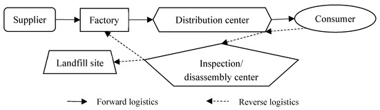
Figure 1.
Closed-loop logistics network structure.
Government reward and punishment revenue and expenditure are associated with enterprises obtaining initial and free carbon emission quotas from carbon emission agencies based on their size and historical carbon emissions. If the actual emissions exceed the quota they will be punished, which is the cost of punishment. However, the government will provide certain rewards which will benefit enterprises if the carbon emissions produced are below certain levels [4]. The revenue and expenditure of government rewards and penalties are mainly based on the amount of carbon dioxide emitted by enterprises in production and related operations. Therefore, the calculation of carbon emission trading revenue and expenditure of remanufacturing logistics networks must be based on the calculation of carbon dioxide emissions. The main sources of carbon dioxide emissions from logistics networks include the following:
- (1)
- The amount of carbon dioxide emitted as a result of energy consumption during the operation of each center, that is, the carbon emissions during the operation process within the facilities. This type of carbon emission is mainly generated by electricity consumption, fuel consumption, and heat consumption. This study only considers the carbon emissions generated by electricity consumption;
- (2)
- The amount of carbon dioxide emissions from energy consumption during transportation between centers. Due to differences in factors, such as vehicle weight [16], transportation distance [23], road slope, and road congestion, the carbon emissions generated as a result of fuel consumption vary. This study only considers vehicle weight and transportation distance. In general, the emission of carbon dioxide is directly proportional to energy consumption.
In actual production operations, due to the interference of uncertain factors, enterprise managers cannot accurately grasp the changes in the remanufacturing market. Therefore, this study assumes that certain parameters are subject to uncertainty and the changes in the parameters are represented by trapezoidal fuzzy numbers [32].
Under the above conditions, this study aims to minimize the sum of production costs, transportation costs, fixed operating costs, landfill costs, and government rewards and punishments in the case of uncertain demand. The problem of facility location selection and transportation route selection between facility nodes in closed-loop logistics networks is further studied. Using fuzzy programming methods, a necessity-based fuzzy programming model for closed-loop logistics networks is established to further assist with decision-making.
3.2. Model Assumptions and Symbols
The following assumptions were made during this research: (1) the closed-loop logistics in this article belongs to strategic decision making; therefore, a single product was considered within a cycle, such as two years or even longer; (2) due to limitations in land resources, the number and processing capacity of each facility are limited; (3) due to the long-term nature of strategic decisions, the recovery rate and landfill rate are both determined; (4) due to its impact on the environment, products that cannot be repaired after recycling will be landfilled considering the location of the landfill site; and (5) without losing generality, products can be recycled in consumer areas and there is a demand for recycled products in consumer areas. The symbols required for the model in this article can be defined as follows (Table 1, Table 2 and Table 3).

Table 1.
Definition of set.
Table 2.
Model parameters.
Table 3.
Decision Variables.
3.3. Objective Function and Constraints of the Fuzzy Optimization Model
This article constructs a necessity-based fuzzy programming model [31,32] where the best solution for necessity is to make all possible solutions solvable to be optimal. Using necessity transformation is more meaningful in meeting opportunity constraints. Thus, the necessity-based fuzzy opportunity-constrained programming model M1 can be constructed as follows.
Firstly, carbon emissions are relevant to energy consumption. To simplify the model, for the carbon emissions during transportation, this study mainly considers two factors (i.e., actual loading capacity and transportation distance) and assumes that carbon emissions are directly proportional to transportation distance. If a vehicle needs to depart, it will generate fixed energy consumption so it is assumed that carbon emissions are proportional to the number of vehicles. Generally, when the transportation volume is less than or equal to the loading capacity of a vehicle, a vehicle can complete transportation. When the transportation volume exceeds the loading capacity of one vehicle, multiple vehicles are required. Therefore, when the first vehicle is fully loaded, the loading capacity of the -th vehicle is the balance between the total transportation volume remaining and the loading capacity. The carbon emissions inside the facility are the sum of the fixed carbon emissions of the facility and the carbon emissions of each facility when processing products, as shown later in the left-hand end of Equation (15).
Then, this study considers the goal of designing a closed-loop logistics network to minimize the total logistics cost. According to the problem description, the total cost consists of production costs, transportation costs, fixed operating costs, landfill costs, and carbon emission rewards and penalties. The objective function can be expressed as follows:
According to the model assumptions, the decision variables of the objective function need to meet the following constraints:
Among them, Equations (2)–(7) are the capacity constraints and Equations (3)–(7) indicate that the necessity of each node’s capacity should be greater than or equal to , respectively. Equations (8)–(13) represent the flow balance constraints for all the locations within the closed-loop supply chain. Equation (14) indicates that the necessity of meeting consumer needs cannot be less than . Equation (15) models carbon dioxide emissions throughout supply chain operations where the operator represents rounding up. Equation (16) represents the cardinality constraints for 0–1 variables. Equation (17) represents the cardinality constraints for non-negative integers. Equation (18) represents the cardinality constraints for the real numbers ranging between 0 and 1.
Since is a decision variable and cannot be directly rounded to , adding variable , letting , yields
The treatment of , , , , , and can be conducted in a similar fashion and variables , , , , , and will be added to the model as well. Therefore, Equation (15) will be replaced with Equation (22) as follows:
3.4. Defuzzified Model Formulation
According to [31,32], if is a fuzzy variable, its membership function is , and if is a real number, then the necessity measure can be represented as follows:
The expected value of fuzzy variable is
In this article, is represented by trapezoidal fuzzy numbers, namely , . According to Equation (24), the expected value of is and according to Equation (23) its necessity distribution can be expressed as follows:
According to Equations (25) and (26), if is a trapezoidal fuzzy number and for a given confidence level , then
According to the above analysis, model M1 can be transformed into an equivalent and deterministic model M2 as follows:
s.t. Equations (2), (8)–(13), and (16)–(21)
Among them, Equations (30)–(34) are nonlinear and need to be linearized. Letting , Equation (30) can be replaced with the following relationships:
Similarly, letting , , , and , then Equation (31) can be replaced with the following relationships:
Equation (32) can be replaced with the following relationships:
Equation (33) can be replaced with the following relationships:
Equation (34) can be replaced with the following relationships:
4. Solution Method
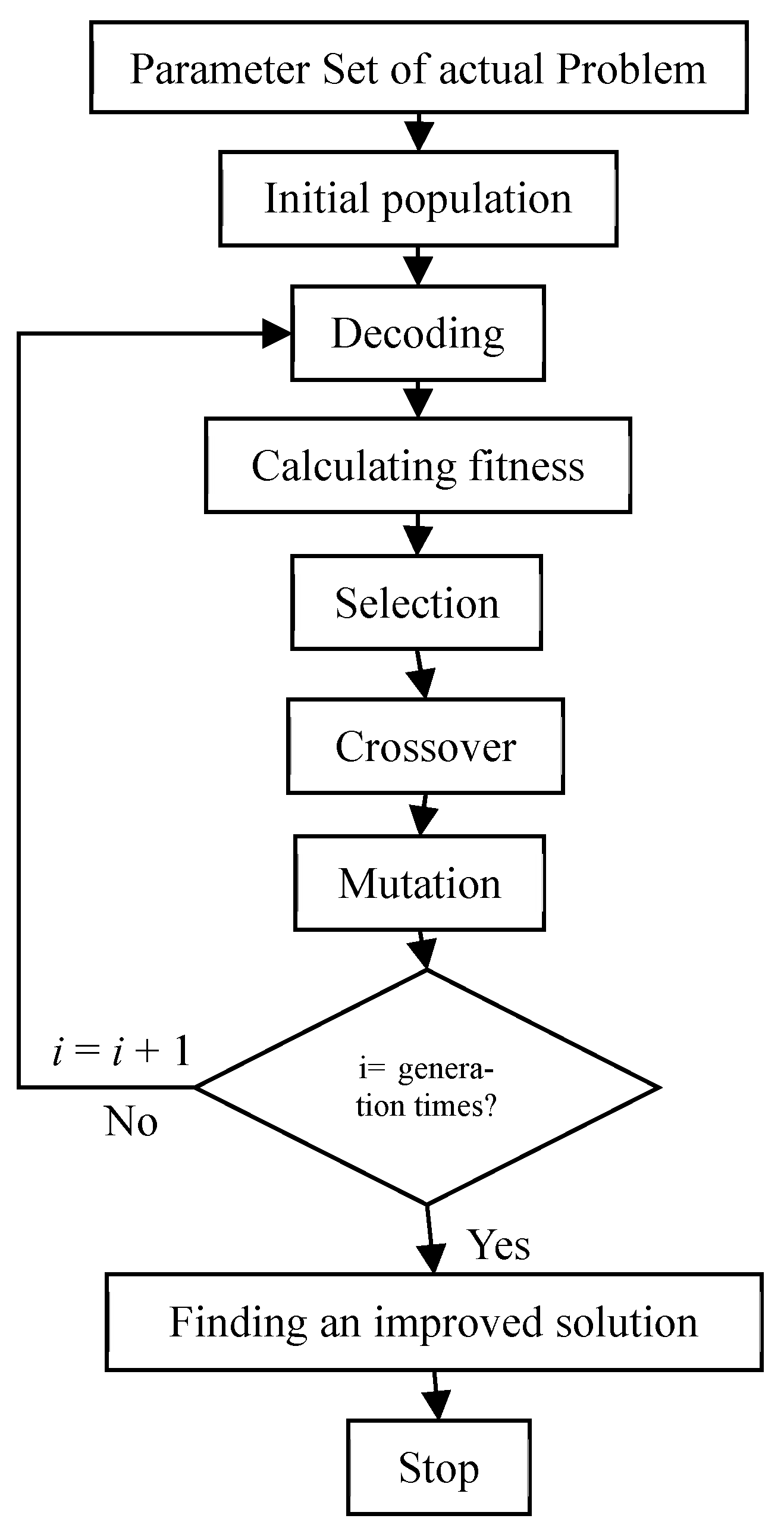
This study proposes a variant priority encoding genetic algorithm (VPGA) to solve the problem formulated using the optimization model M2. The algorithm flow is shown in Figure 2 and its main steps are further discussed in this section of the manuscript.

Figure 2.
VPGA algorithm solution flow chart.
4.1. Encoding and Decoding Operation
This study adopts a variant priority-based encoding method which has the advantage that there is no need to repair the encoded solutions (i.e., individuals or chromosomes) during the subsequent steps of the search process after the solution initialization. The variant priority-based encoding method developed in this study is inspired by the encoding method proposed by [45] and directly captures the specific characteristics of the decision problem studied herein. The main steps of the individual encoding operation are summarized in Algorithm 1.
| Algorithm 1: Encoding procedure adopted within the proposed VPGA algorithm |
| Input: |
| : Total number of suppliers |
| : Total number of factories |
| : Total number of distribution centers |
| : Total number of consumption areas |
| : Total number of inspection/disassembly centers |
| : Total number of landfill sites |
| Output: |
| : realization degree |
| : priority matrix, where , , , , , . |
| For q = 1, 2, …, 6 |
| Step 1: Generate as a random number between [0.5, 1] |
| End |
| Step2: Randomly arrange 1 to numbers on the Empty matrix to obtain a matrix with rows and columns and let = . |
| Step3: Randomly arrange 1 to numbers on the Empty matrix to obtain a matrix with rows and columns and let = . |
| Step4: Randomly arrange 1 to numbers on the Empty matrix to obtain a matrix with rows and columns and let = . |
| Step5: Randomly arrange 1 to numbers on the Empty matrix to obtain a matrix with rows and columns and let = . |
| Step6: Randomly arrange 1 to numbers on the Empty matrix to obtain a matrix with rows and columns and let = . |
| Step7: Randomly arrange 1 to numbers on the Empty matrix to obtain a matrix with rows and columns and let = . |
| Step8: Randomly arrange 1 to numbers on the Empty matrix to obtain a matrix with rows and columns and let = . |
| Note: The symbols used in this operation are independent of the symbols used in the model. |
Based on the above individual encoding operations and the characteristics of optimization model M2 proposed in this study, the decoding operation will be applied afterwards. The main steps of the individual decoding operation are summarized in Algorithm 2.
| Algorithm 2: Decoding procedure adopted within the proposed VPGA algorithm |
| Input: |
| : Set of starting points |
| : Set of destinations |
| : The ability of starting point , |
| : The demand for destination , |
| : priority matrix |
| Output: |
| : Transportation volume from node to node |
| Step1: let |
| While |
| Step2: |
| Step3: Update demand and capacity: , |
| Step4: If then If then |
| Step5: If then output else return to Step2 |
| End |
An example of a decoding procedure used by the VPGA algorithm is shown in Table 4 and Table 5. In particular, Table 5 shows the iterative decoding process based on the input data given in Table 4.
Table 4.
Example explanation of a priority matrix.
Table 5.
Decoding process tracking table.
Based on the provided example, the decoding procedure can be summarized in a more compact form which is presented in Algorithm 3.
| Algorithm 3: Decoding procedure adopted within the proposed VPGA algorithm |
| Input: : realization degree |
| : priority matrix |
| Output: |
| Step1: Calculate using Algorithm 2 |
| Step2: Calculate using Algorithm 2 |
| Step3: Calculate using Algorithm 2 |
| Step4: Calculate using Algorithm 2 |
| Step5: Calculate using Algorithm 2 |
| Step6: Calculate using Algorithm 2 |
| Step7: Calculate using Algorithm 2 |
4.2. Fitness and Selection Operations
The calculation formula for fitness of solutions was set as follows: fitness = (1/individual objective function value). The roulette wheel selection method was used as a selection mechanism. Furthermore, the elitist strategy was applied as well to make sure that the best individual will be present in the next generation of the algorithm before applying crossover, mutation, and selection operators.
4.3. Crossover Operation and Mutation Operation
- (1)
- The crossover operation used in the VPGA algorithm is based on a well-known single-point crossover method.
According to Algorithm 1, a feasible individual can be obtained including the implementation degrees {} and the priority matrix {}. Then, the crossover operation can be conducted based on the following steps:
Step 1: Randomly divide all the parental chromosomes into pairwise groups.
Step 2: Randomly select an integer between [1, 6] and an integer between [1, 7].
Step 3: Exchange the values of {} from to 6 between two individuals and exchange the values of {} from to 7 to obtain two individuals.
- (2)
- The method of mutation operation (exchange mutation or swap mutation) can be conducted based on the following steps:
Step 1: For {}, a random element , randomly select two different integers and from among .
Step 2: Exchange the priority number of and .
An example of a mutation operation is presented in Table 6. In this example, two numbers, (i.e., 3 and 8 that are highlighted in bold) are selected at random and then exchanged.
Table 6.
Mutation operation example.
5. Numerical Experiments
5.1. Input Data Generation
To demonstrate the effectiveness of the VPGA algorithm, this study randomly generated four numerical examples based on the data presented in Table 2 and Table 7. The VPGA algorithm, pGA algorithm [44], and CPLEX12.8 were used to solve the examples and the results obtained by the solution approaches were further analyzed in detail. The VPGA and pGA codes were written in MATLAB 7.0 and the computational experiments were executed on a computer with an Intel (R) Core (TM) i5 2.53 GHz processor, 4 GB of memory, and a 64-bit system. Based on a preliminary parameter tuning analysis, the crossover rate of VPGA and pGA algorithms was set to 60–70% and the mutation rate was set to 10–15%. The carbon emission limits were restricted to 12,529,000, 23,533,000, 45,944,000, and 89,529,550 in the developed problem instances.
Table 7.
Scale of test instances (unit: units).
5.2. Evaluation of the Candidate Solution Approaches
All the considered solution approaches were executed for the four generated test instances and the results are shown in Table 8 where the error rate was estimated as follows: (GA best value—CPLEX best value)/CPLEX best value. The bold font was used to show best objective function value recorded. Notably, the population size and the number of generations were increased for VPGA and pGA for larger problem instances to discover superior solutions (both population size and number of generations were set based on preliminary parameter tuning runs). As shown in Table 8, for test instance 1, the best values obtained by VPGA, pGA, and CPLEX were the same, indicating that VPGA and pGA could be suitable for small-scale problems. For test instances 2 and 3, the best values obtained by VPGA were larger than those obtained by CPLEX, reflecting a decrease in the accuracy of VPGA when solving larger-scale problems. However, the best value error between VPGA and CPLEX was less than 1%. As for test instance 4, the best value obtained by VPGA was superior to CPLEX. Although the VPGA computational time was increasing with the problem size, the best values obtained by VPGA became more and more competitive when comparing to CPLEX and pGA. The CPLEX computational time became prohibitive for large-scale problem instances (i.e., test instance 4). Therefore, from the above analysis, the VPGA algorithm has a high degree of accuracy and is competitive in terms of computational time when comparing to CPLEX.
Table 8.
Comparison and analysis of results obtained by VPGA, CPLEX, and pGA.
A further analysis of Table 8 shows that for test instance 1, the best values obtained by VPGA and pGA algorithms were the same. For test instances 2–4, the best values obtained by VPGA were smaller than those obtained by pGA and its running time was shorter than that of pGA. Moreover, as the problem size enlarges, the computational time increases faster for pGA when comparing to VPGA. In addition, VPGA was found to be more prone to jumping out of the local optimal solutions and resulting in higher quality solutions (see Table 8). Therefore, it can be concluded that VPGA is more advantageous than pGA in terms of solution quality and computational time, especially for large-size test instances.
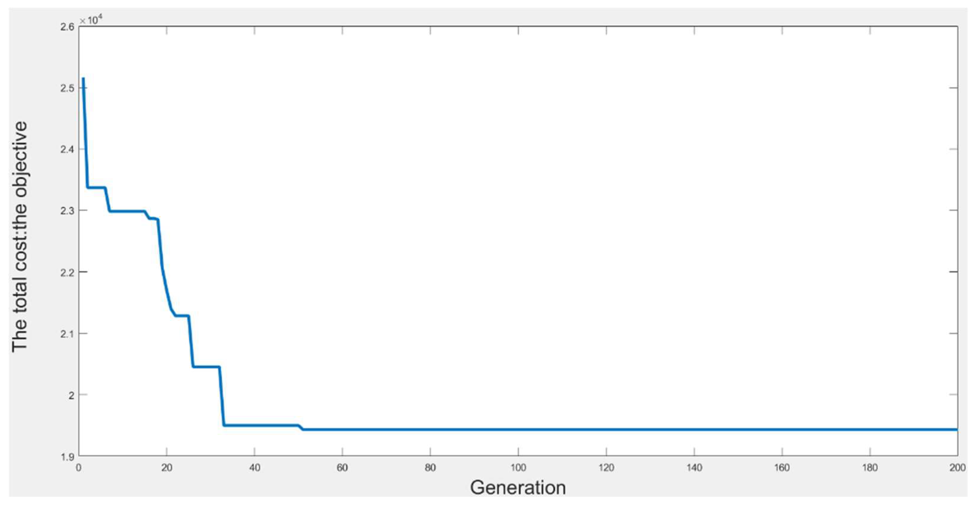
Figure 3 shows the detailed distribution of the objective values obtained using VPGA in the different generations of test instance 1. This graph can be used to investigate the convergence and validity of the VPGA algorithm. In actual life production, logistics enterprises often need to solve the problem of large-scale transportation route arrangement. Low-cost transportation plans have to be obtained as soon as possible so that logistics costs will remain low. General optimization software (e.g., CPLEX, GUROBI, and MOSEK) may take a long time to find a solution and, therefore, are not considered as practically efficient. Based on the convergence patterns presented in Figure 3, the genetic algorithm based on priority encoding proposed in this paper can obtain good-quality solutions fairly quickly (i.e., within the first 50–60 generations). Hence, the proposed algorithm could be effectively used by practitioners to design the most sophisticated closed-loop supply chains.
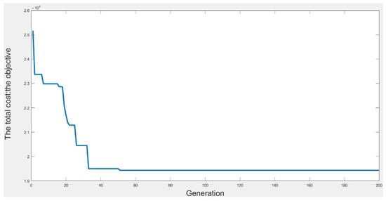
Figure 3.
The VPGA convergence patterns for test instance 1.
5.3. Sensitivity Analysis and Managerial Insights
This study uses test instance 1 to conduct a detailed sensitivity analysis for the network model [18]. The processing capabilities of the suppliers were set to 500, 650, and 390. The fixed operating costs of the factory were set to 1800, 900, 2100, 1100, and 900 with fixed carbon emission coefficients of 2,345,000, 2,390,000, 2,360,000, 2,330,000, and 2,375,000, respectively. The fixed operating costs of the distribution center were set to 1000, 900, and 1600 and their fixed carbon emission coefficients comprised 84,500, 84,750, and 84,250, respectively. The fixed operating costs of the testing/dismantling center were set to 100 and 110 and their fixed carbon emission coefficients comprised 845,000 and 847,500, respectively. The fixed operating costs of landfill sites were set to 370, 390, and 200 and their fixed carbon emission coefficients comprised 830,000, 827,500, and 832,500, respectively. The transportation cost per kilometer per unit of products was assumed to be 1 CNY/kilometer. The carbon emission coefficients of unit products processed in factories, distribution centers, testing/dismantling centers, and landfill sites were set to 975, 350, 760, and 530, respectively. The other relevant data used in the experiments are shown in Table 9, Table 10, Table 11, Table 12, Table 13, Table 14 and Table 15.
Table 9.
Transportation distance between suppliers and factories (km).
Table 10.
Transportation distance between factories and distribution centers (km).
Table 11.
Transportation distance between distribution centers and consumption areas(km).
Table 12.
Transportation distance between consumption areas and distribution centers(km).
Table 13.
Transportation distance between distribution centers and inspection/disassembly centers (km).
Table 14.
Transportation distance between inspection/disassembly centers and factories(km).
Table 15.
Transportation distance between inspection/disassembly centers and landfill sites s (km).
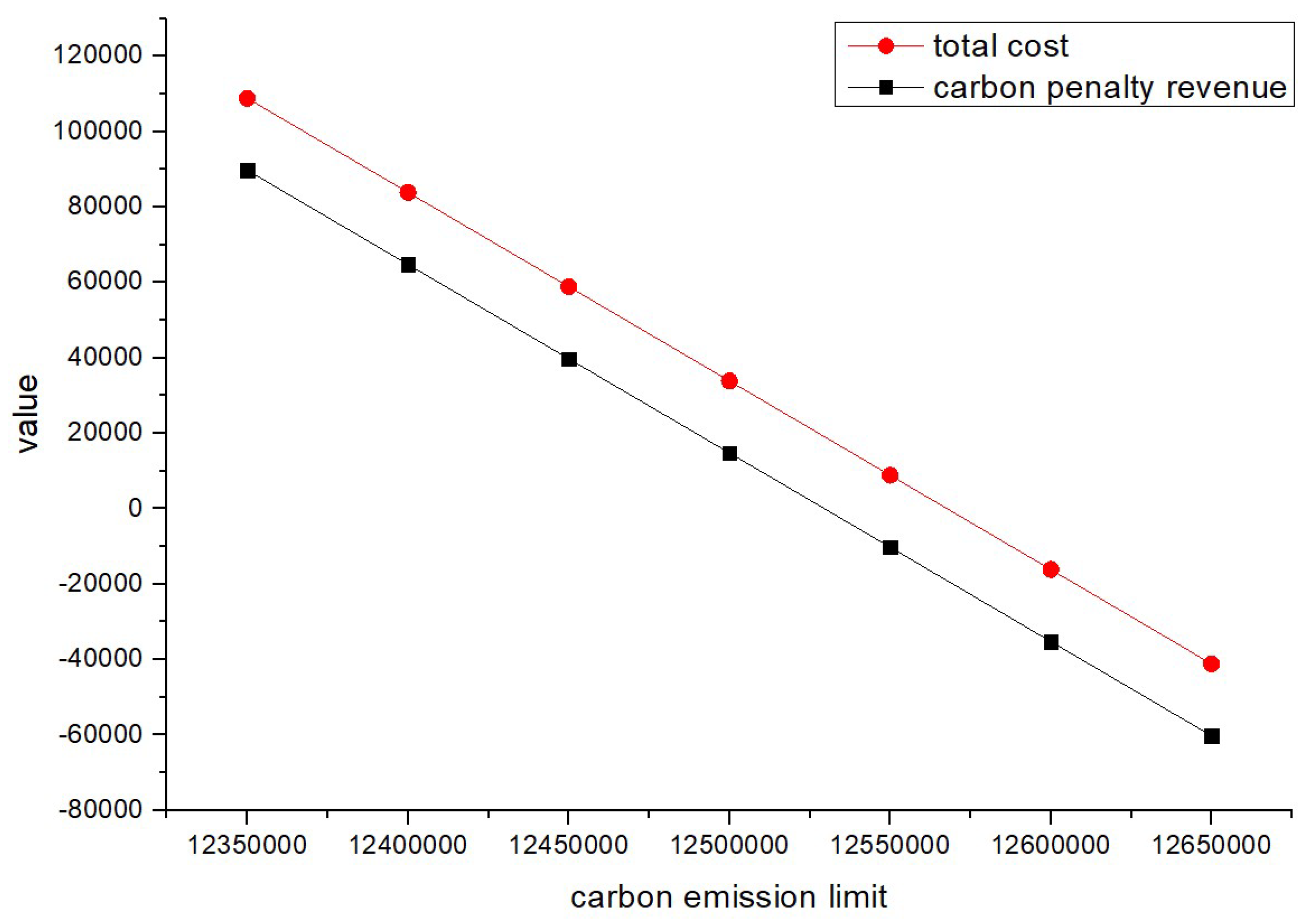
To analyze the impact of carbon emission limits on the model results and test the stability of the logistics network, carbon emission limits were set at 12,350,000, 1,240,000, 12,450,000, 12,500,000, 12,550,000, 12,600,000, and 12,650,000. The developed VPGA algorithm was used to solve the problem for all the scenarios of carbon emission limits assuming that . The carbon penalty revenue and total cost of the network are presented in Table 16 under each carbon emission limit where the negative values represent the revenue. Moreover, the corresponding facility locations and transportation volumes which represent the number of shipments between the nodes are shown in Table 17 and Table 18, respectively, under each carbon emission limit. In order to better illustrate the results, Figure 4 and Figure 5 were also made based on the data reported in Table 16 and Table 18, respectively (the meaning of the graph in Figure 5 is consistent with the meaning of the graph in Figure 1).
Table 16.
Changes in the carbon penalty/revenue and the total cost for different carbon emission limits.
Table 17.
Facilities selection.
Table 18.
Number of shipments.

Figure 4.
Changes in total cost and carbon penalty/revenue (pu = re = 0.5).
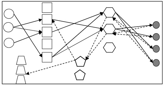
Figure 5.
Logistics network structure.
Based on the results reported in Table 17, factories 2, 3, and 5, distribution centers 1 and 2, testing/dismantling center 1, and landfill site 2 were selected for all the considered carbon emission limit scenarios. Therefore, the carbon emission limit changes did not influence the decisions regarding the facility site selection. Furthermore, the transportation volumes between facilities remained the same for all the considered carbon emission limit scenarios as well (as shown in Table 18). The total cost and carbon revenue/penalty (as shown in Figure 4) both decrease with the increase in carbon emission quotas as the increase in carbon emission quotas increases the number of carbon emissions below the quota, transforming the carbon reward and punishment revenue and expenditure from punishment to reward, thereby reducing the total cost. However, the logistics network structure (as shown in Figure 5) has remained unchanged, indicating that the network is relatively stable. For logistics enterprise managers, a stable network is exactly what they are looking for.
Under the fuzzy conditions set in this example, the constraint satisfaction level was assumed to 0.5, indicating a 50% chance of meeting the constraint conditions in the event of a change in carbon emission limits. Although enterprise managers are eager to improve the certainty of decision making, that is, to improve the level of constraint satisfaction; in real life, there are many uncertain parameters and the set constraint conditions cannot be fully satisfied. Furthermore, an excessively conservative approach against uncertainties can result in a very costly supply chain design. Therefore, a satisfaction level of 0.5 for fuzzy parameters could be considered as reasonable from a practical standpoint. Simultaneous decision making carries risks, especially in fuzzy environments where it is difficult for enterprise managers to judge the correctness of a solution. The fuzzy programming method used in this model can be helpful to decision makers in such cases.
In summary, the fuzzy programming model proposed in this study is in line with reality. In the case of fuzzy parameters, the change in carbon emission limits has no significant impact on the location and level of logistics network nodes as well as the transportation routes between the nodes. This indicates that when external parameters change, the model’s solution maintains a certain level of satisfaction conservation and can be effectively applied to the entire logistics network, making it a reasonable and applicable strategic solution. The decisions provided by the model reflect stability and practicality while also providing a decision-making basis for enterprise managers which is suitable for the development of the enterprise.
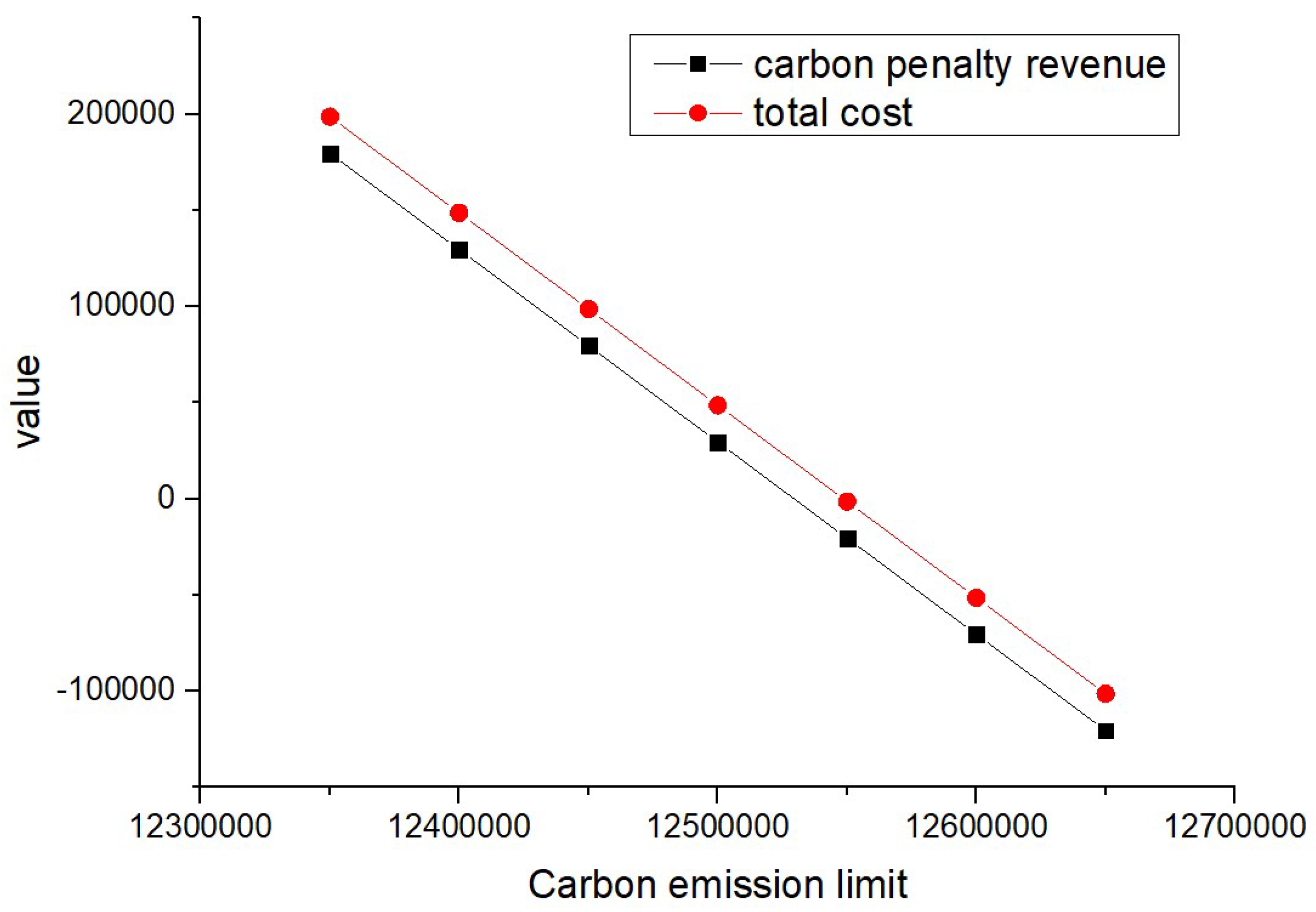
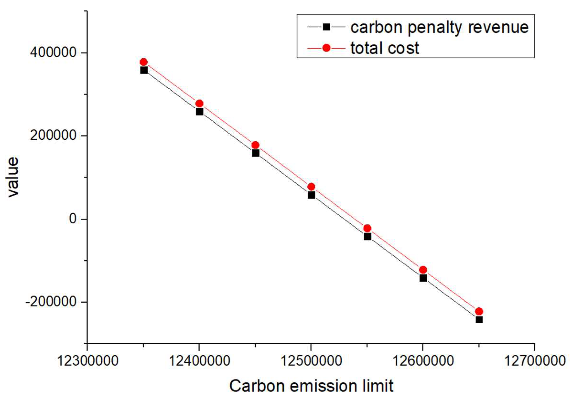
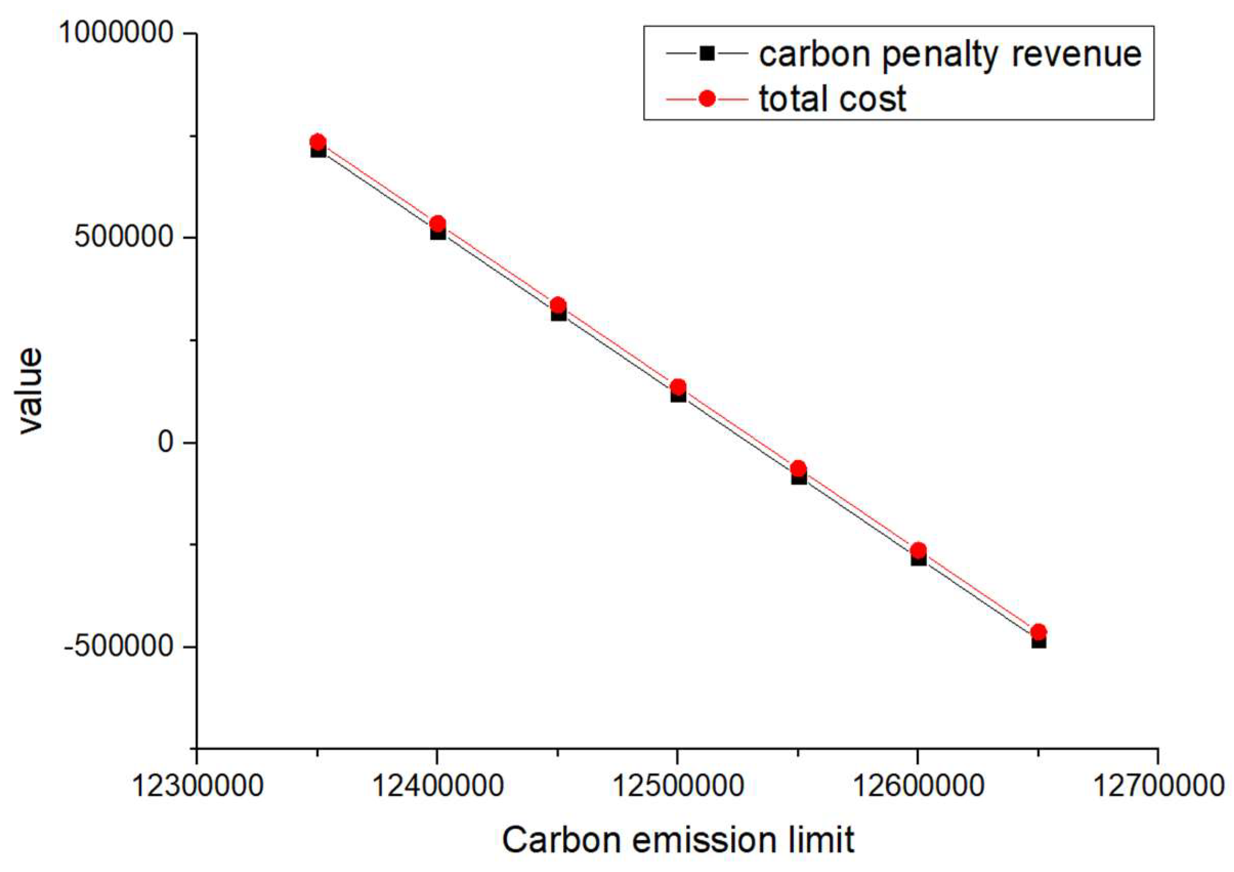
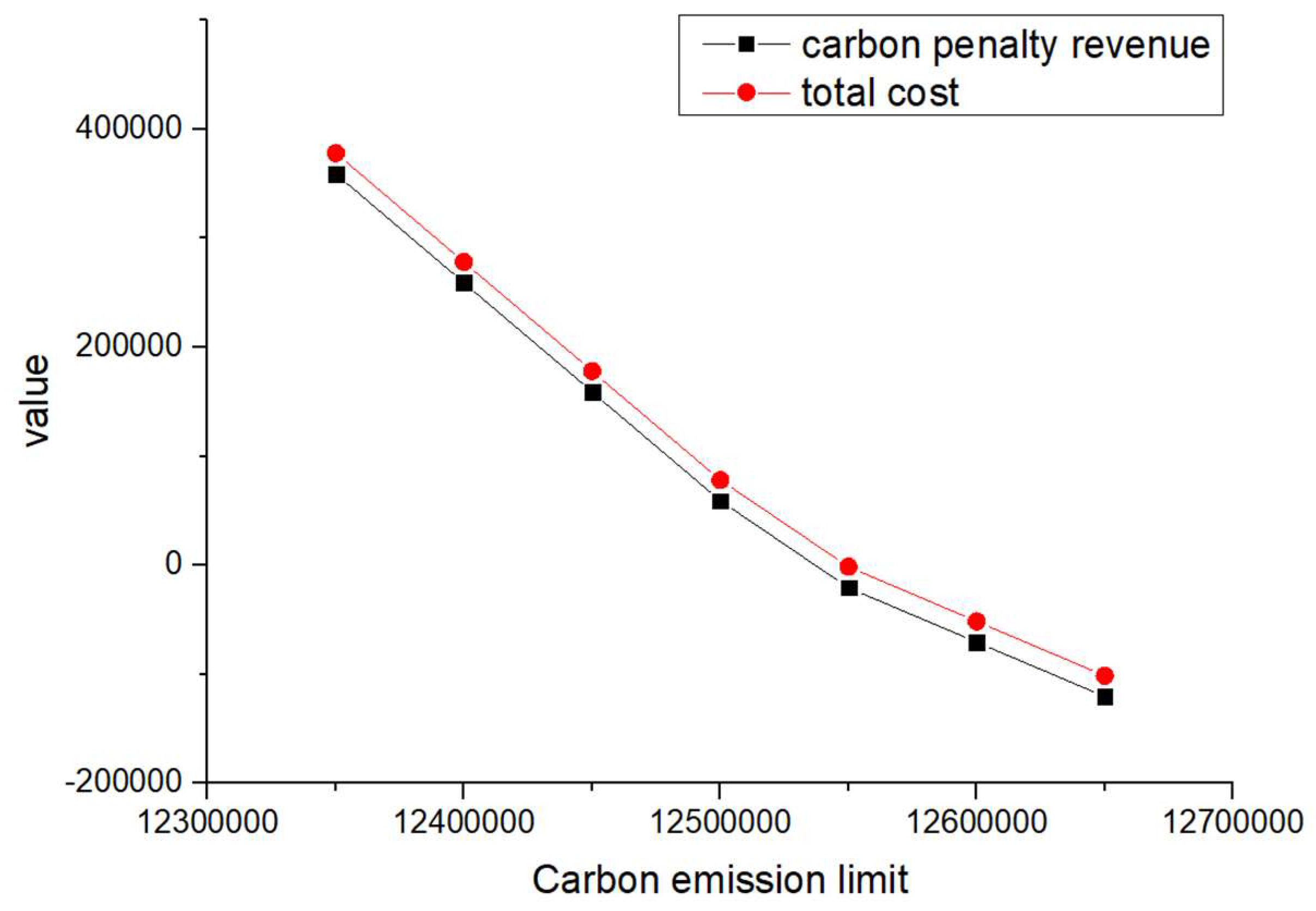
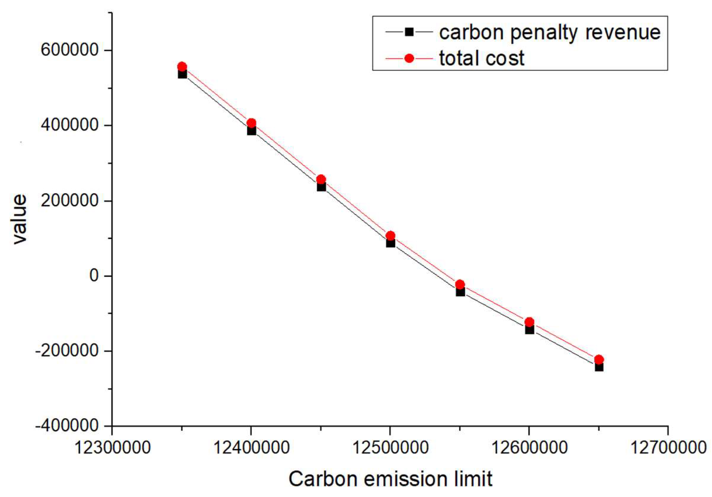
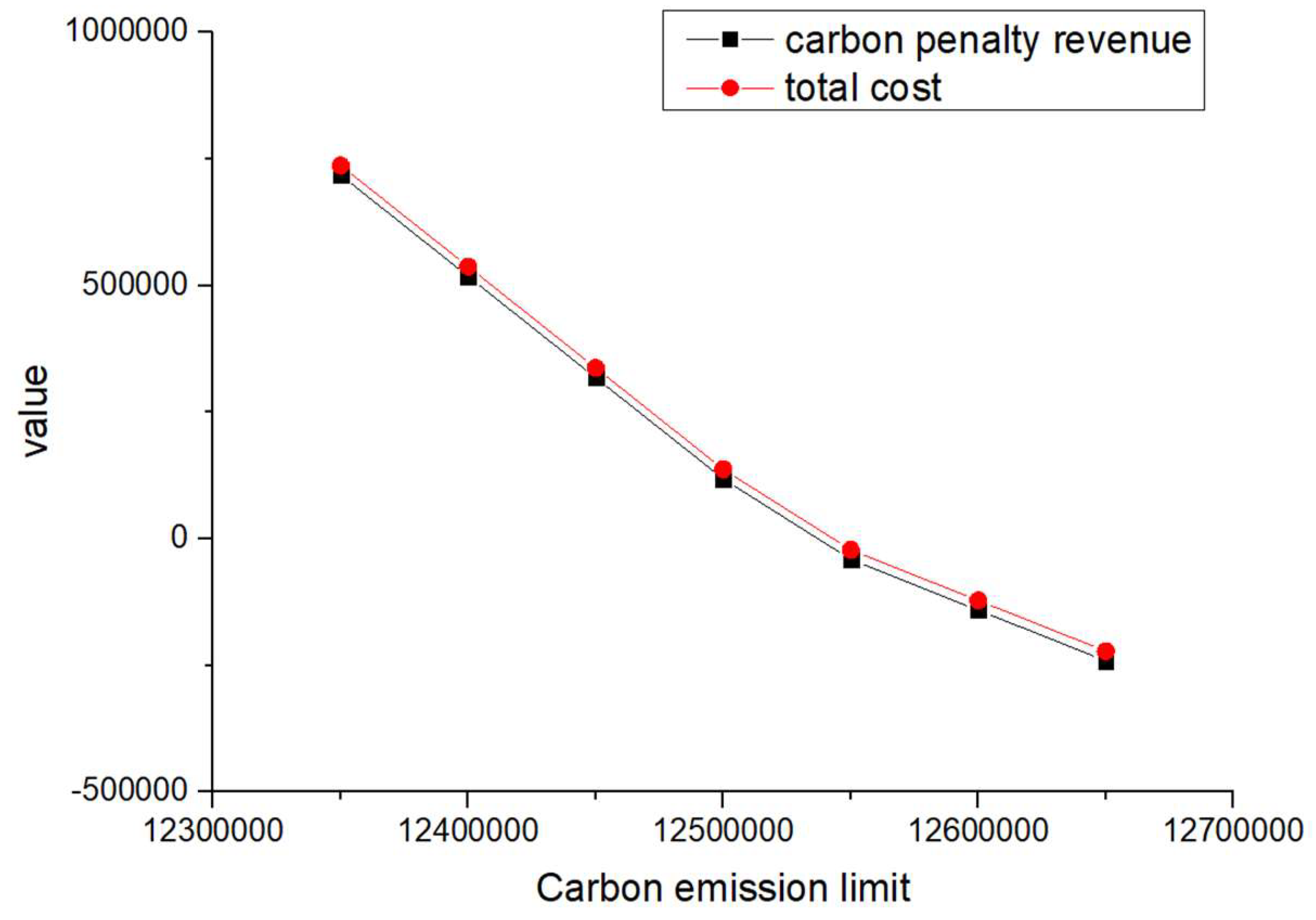
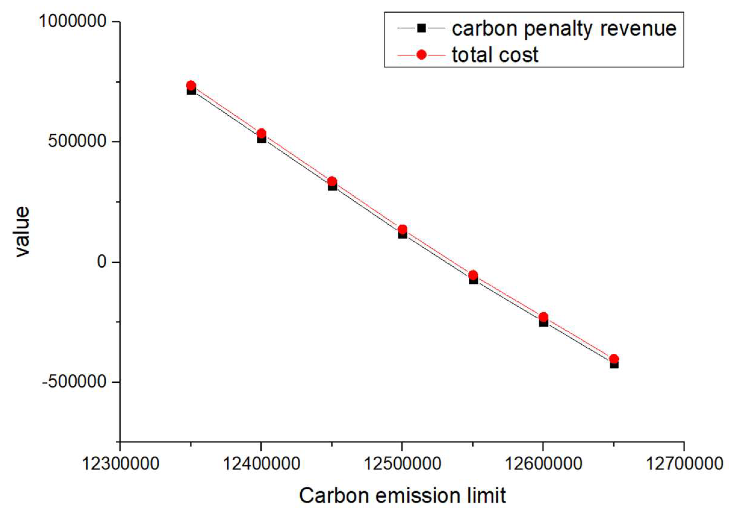
In order to analyze the impact of the penalty cost and reward amount per unit of carbon emissions on the carbon penalty revenue and total cost, different values of and were considered during the sensitivity analysis, as shown in Table 19. The developed VPGA algorithm was executed for all the considered unit penalty cost and reward amount values; the corresponding changes in total cost and carbon penalty/revenue are shown in Figure 6, Figure 7, Figure 8, Figure 9, Figure 10, Figure 11, Figure 12 and Figure 13.
Table 19.
Changes in penalty cost (pu) and reward amount (re) per unit of carbon emissions.

Figure 6.
Changes in total cost and carbon penalty revenue (= = 1).
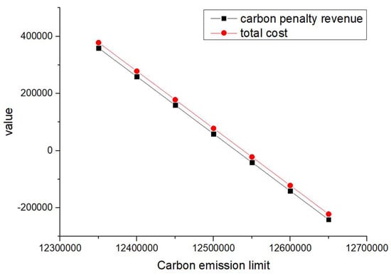
Figure 7.
Changes in total cost and carbon penalty revenue (= = 2).
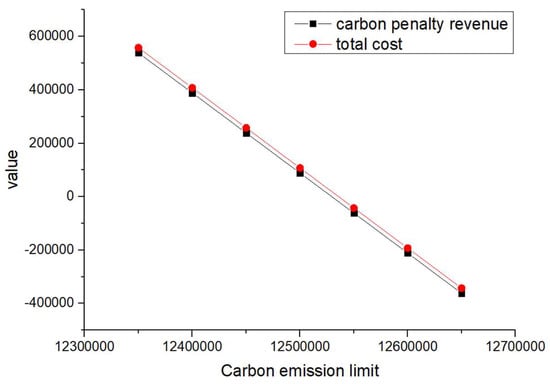
Figure 8.
Changes in total cost and carbon penalty revenue (= = 3).
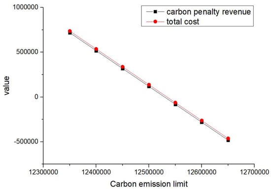
Figure 9.
Changes in total cost and carbon penalty revenue (= = 4).
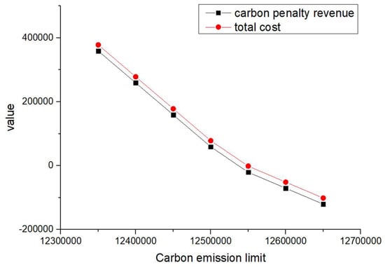
Figure 10.
Changes in total cost and carbon penalty revenue ( = 2 = 1).
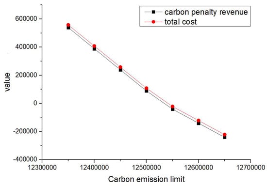
Figure 11.
Changes in total cost and carbon penalty revenue ( = 3 = 2).
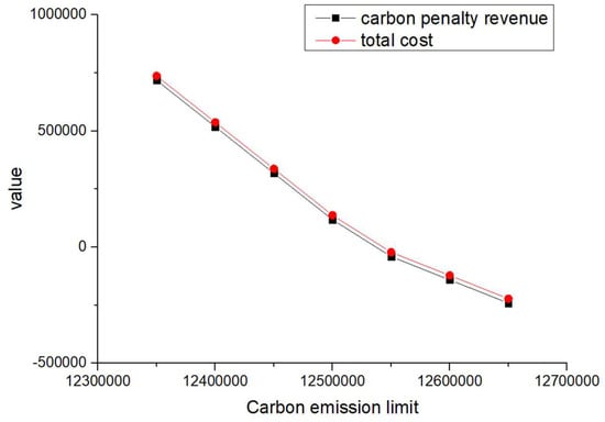
Figure 12.
Changes in total cost and carbon penalty revenue ( = 4 = 2).
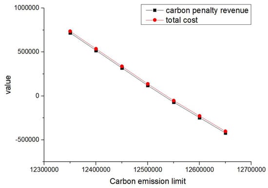
Figure 13.
Changes in total cost and carbon penalty revenue ( = 4 = 3.5).
When and are equal and their values increase from 1 to 4 (such as scenarios 1–4) and when is greater than and its value increases (such as scenarios 5–8), the total cost and carbon reward and penalty revenue and expenditure decrease with the increase in carbon emission quotas. From a vertical perspective, the difference in their values decreases when the values of and increase and carbon emission costs account for a larger proportion compared to logistics costs excluding carbon emission costs. Such findings may encourage enterprises to consider the impact of carbon punishment on their revenue and expenditure projections when conducting logistics activities, thereby inducing them to manage toward green supply chain practices.
In addition, when and are equal and their values increase from 1 to 4 (such as scenarios 1–4), the carbon penalty revenue and total cost decrease linearly with the increase in carbon emission limits. When is greater than and its value increases (such as in scenarios 5–8), the carbon penalty revenue and total cost decrease with the increase in carbon emission limits, showing a nonlinear and convergent state. The first scenario states that equality will lead to an infinite increase in profits for enterprises as their carbon emissions become better and better. However, this is a misalignment with economic principles and the original intention of the government in formulating policies. In the second case, when is greater than , it is in line with the punishment effect in the government’s emission reduction policies and its convergence state is also in line with the situation where a certain economic activity will not increase profits indefinitely. However, when a certain carbon emission limit is given and the company’s profits no longer change, this carbon emission limit should be further allocated to that company. Therefore, the government needs to determine the value of carbon emission quotas allocated to , , and enterprises, where is greater than .
At present, global climate change, environment, and energy are showing a trend of gradual deterioration. As such, in future development, the world needs to be based on the concept of low-carbon development to ensure the effectiveness of environmental protection. The current logistics industry has always been an important component of energy and carbon emissions. Hence, in the future development of the logistics industry, a gradual transformation into a low-carbon logistics industry will be essential. The methodology proposed in this study could be used to achieve the future environmental goals when planning complex closed-loop supply chain networks.
6. Conclusions
In recent years, due to concerns about the environment and constraints imposed by government reward and punishment mechanisms, manufacturing companies have been trying to reuse and remanufacture their products to reduce pollution caused by product scrapping. Considering that recycling old products can bring enormous economic and environmental benefits, current research proposes the optimization of facility location in closed-loop supply chains in low-carbon environments. The proposed closed-loop supply chain network consists of suppliers, factories, distribution centers, consumption areas, dismantling centers, and landfill sites. In the current research, the demand for products, facility capacity, transportation cost per unit of product per kilometer, landfill cost, unit penalty cost, and reward amount of different customers are considered uncertain and are assumed to be fuzzy numbers. A mixed integer programming model was proposed to minimize the total cost of the network, including production costs, transportation costs, fixed operating costs, landfill costs, and carbon emission rewards and penalties.
Based on the characteristics of the model, a new encoding method based on variant priority encoding was proposed and applied to the framework of genetic algorithms. Finally, based on comparative analysis with the precise optimization method (CPLEX) and the traditional priority-based genetic algorithm, the effectiveness of this algorithm was demonstrated through several computational examples. The results of numerous experiments indicate that even for large-scale numerical examples, the proposed algorithm can provide high-quality solutions faster. The applicability of the model was demonstrated through a sensitivity analysis which was conducted by changing some of the uncertain parameters of the model. The results of this study are expected to provide scientific support for relevant supply chain enterprises, policymakers, industrial practitioners, environmental scientists, and stakeholders.
On the basis of the original problem, this article considers the selection of landfill sites to make the network structure more complete and adds factors such as carbon emission limits and government rewards and punishments to the model from the government’s perspective, making the closed-loop logistics network more practical. In addition, the necessity setting for uncertain situations reflects the optimal solution for closed-loop logistics network problems which means that all possible solutions are solvable to be optimal. Therefore, adopting necessity transformation is more meaningful in meeting opportunity constraints. Finally, the impact of closed-loop logistics on social management includes (1) reducing logistics costs, reducing resource waste, reducing logistics costs, and improving transportation efficiency and (2) energy conservation and closed-loop logistics systems that can greatly reduce energy waste, fuel consumption, and energy consumption. In traditional logistics systems, goods need to be packaged and cleaned which generates a large amount of waste and energy waste. In closed-loop logistics, both transportation facilities and packaging items can be reused to reduce energy consumption.
The current research can be further expanded in several aspects. In the future, our goal in a low-carbon environment is to minimize costs and conduct joint optimization research in a sustainable direction, capturing various criteria in multi-objective settings. In addition, the algorithm proposed in this study has specific universality and can be widely applied in logistics network models in the next step. Last but not least, the proposed encoding scheme can be investigated for other types of metaheuristics (e.g., ant colony optimization, particle swarm optimization, grey wolf optimizer, and others).
Author Contributions
Conceptualization: B.L. and Q.C. Methodology: B.L., Q.C. and Y.-y.L. Formal analysis and investigation: B.L., K.L. and Q.C. Writing—original draft preparation: B.L. Writing—review and editing: B.L., Y.-y.L., K.L. and M.A.D. Supervision: Q.C., Y.-y.L. and M.A.D. All authors have read and agreed to the published version of the manuscript.
Funding
This research was funded by a major project of Fujian Provincial Department of Education (JAT220181), research on Building a New Highland for Marine Scientific Research and Innovation in Xiamen (Xiamen Society Scientific Research [2023] No. C08), research platforms and projects of Guangzhou Basic Research Program Basic and Applied Basic Research Project (SL2023A04J00414), higher education institutions of Guangdong Provincial Department of Education (2022KQNCX064), the Educational Science Planning Project of Guangdong Provincial Department of Education (Higher Education Project) (2021GXJK074), and the Discipline Construction Project of Guangzhou Jiaotong University (K52022026).
Institutional Review Board Statement
This article does not contain any studies with human participants or animals performed by any of the authors.
Informed Consent Statement
Not applicable.
Data Availability Statement
The datasets used and/or analyzed during the current study are available from the corresponding author on reasonable request.
Conflicts of Interest
The authors declare no conflict of interest.
References
- Xu, Z.; Elomri, A.; Liu, W.; Liu, H.; Li, M. Robust global reverse logistics network redesign for high-grade plastic wastes recycling. Waste Manag. 2021, 134, 251–262. [Google Scholar] [CrossRef] [PubMed]
- Govindan, K.; Soleimani, H.; Kannan, D. Reverse logistics and closed-loop supply chain: A comprehensive review to explore the future. Eur. J. Oper. Res. 2015, 240, 603–626. [Google Scholar] [CrossRef]
- Feng, Y.; Dong, Z. Comparative lifecycle costs and emissions of electrified powertrains for light-duty logistics trucks. Transp. Res. Part D Transp. Environ. 2023, 117, 103672. [Google Scholar] [CrossRef]
- Yi, W.; Zhen, L.; Jin, Y. Stackelberg game analysis of government subsidy on sustainable off-site construction and low-carbon logistics. Clean. Logist. Supply Chain 2021, 2, 100013. [Google Scholar]
- Jafari, H.; Eslami, M.H.; Paulraj, A. Postponement and logistics flexibility in retailing: The moderating role of logistics integration and demand uncertainty. Int. J. Prod. Econ. 2021, 243, 108319. [Google Scholar] [CrossRef]
- Fathollahi-Fard, A.M.; Dulebenets, M.A.; Hajiaghaei–Keshteli, M.; Tavakkoli-Moghaddam, R.; Safaeian, M.; Mirzahosseinian, H. Two hybrid meta-heuristic algorithms for a dual-channel closed-loop supply chain network design problem in the tire industry under uncertainty. Adv. Eng. Inform. 2021, 50, 101418. [Google Scholar] [CrossRef]
- Asghari, M.; Afshari, H.; Al-e-hashem, S.M.J.; Fathollahi-Fard, A.M.; Dulebenets, M.A. Pricing and advertising decisions in a direct-sales closed-loop supply chain. Comput. Ind. Eng. 2022, 171, 108439. [Google Scholar] [CrossRef]
- Gholizadeh, H.; Goh, M.; Fazlollahtabar, H.; Mamashli, Z. Modelling uncertainty in sustainable-green integrated reverse logistics network using metaheuristics optimization. Comput. Ind. Eng. 2021, 163, 107828. [Google Scholar] [CrossRef]
- Kulińska, E.; Kulińska, K. Development of ride-sourcing services and sustainable city logistics. Transp. Res. Procedia 2019, 39, 252–259. [Google Scholar] [CrossRef]
- Salehi-Amiri, A.; Zahedi, A.; Akbapour, N.; Hajiaghaei-Keshteli, M. Designing a sustainable closed-loop supply chain network for walnut industry. Renew. Sustain. Energy Rev. 2021, 141, 110821. [Google Scholar] [CrossRef]
- Rajabi-Kafshgar, A.; Gholian-Jouybari, F.; Seyedi, I.; Hajiaghaei-Keshteli, M. Utilizing hybrid metaheuristic approach to design an agricultural closed-loop supply chain network. Expert Syst. Appl. 2023, 217, 119504. [Google Scholar] [CrossRef]
- Prajapati, D.; Pratap, S.; Zhang, M.; Lakshay; Huang, G.Q. Sustainable forward-reverse logistics for multi-product delivery and pickup in B2C e-commerce towards the circular economy. Int. J. Prod. Econ. 2022, 253, 108606. [Google Scholar] [CrossRef]
- Kim, Y.G.; Chung, B.D. Closed-loop supply chain network design considering reshoring drivers. Omega 2022, 109, 102610. [Google Scholar] [CrossRef]
- Lu, S.; Chen, C.; Wang, Y.; Li, Z.; Li, X. Coordinated scheduling of production and logistics for large-scale closed-loop manufacturing using Benders decomposition optimization. Adv. Eng. Inform. 2022, 55, 101848. [Google Scholar] [CrossRef]
- Ullah, M. Impact of transportation and carbon emissions on reverse channel selection in closed-loop supply chain management. J. Clean. Prod. 2023, 394, 136370. [Google Scholar] [CrossRef]
- Köseli, İ.; Soysal, M.; Çimen, M.; Sel, Ç. Optimizing food logistics through a stochastic inventory routing problem under energy, waste and workforce concerns. J. Clean. Prod. 2023, 389, 136094. [Google Scholar] [CrossRef]
- Mondal, A.; Roy, S.K. Multi-objective sustainable opened- and closed-loop supply chain under mixed uncertainty during COVID-19 pandemic situation. Comput. Ind. Eng. 2021, 159, 107453. [Google Scholar] [CrossRef]
- Wang, H.F.; Hsu, H.W. A closed-loop logistic model with a spanning-tree based genetic algorithm. Comput. Oper. Res. 2010, 37, 376–389. [Google Scholar] [CrossRef]
- Benjaafar, S.; Li, Y.; Daskin, M. Carbon footprint and the management of supply chains: Insights from simple models. IEEE Trans. Autom. Sci. Eng. 2013, 10, 99–116. [Google Scholar] [CrossRef]
- Wang, J.; Lim, M.K.; Tseng, M.L.; Yang, Y. Promoting low carbon agenda in the urban logistics network distribution system. J. Clean. Prod. 2019, 211, 146–160. [Google Scholar] [CrossRef]
- Wang, J.; Wang, Q.; Yu, M. Green supply chain network design considering chain-to-chain competition on price and carbon emission. Comput. Ind. Eng. 2020, 145, 106503. [Google Scholar] [CrossRef]
- Purnomo, M.; Wangsa, I.; Rizky, N.; Jauhari, W.; Zahria, I. A multi-echelon fish closed-loop supply chain network problem with carbon emission and traceability. Expert Syst. Appl. 2022, 210, 118416. [Google Scholar] [CrossRef]
- Hashmi, N.; Jalil, S.; Javaid, S. A multi-objective model for closed-loop supply chain network based on carbon tax with two fold uncertainty: An application to leather industry. Comput. Ind. Eng. 2022, 173, 108724. [Google Scholar] [CrossRef]
- Xiao, G.; Lu, Q.; Ni, A.; Zhang, C. Research on carbon emissions of public bikes based on the life cycle theory. Transp. Lett. 2023, 15, 278–295. [Google Scholar]
- Rahimi, M.; Ghezavati, V. Sustainable multi-period reverse logistics network design and planning under uncertainty utilizing conditional value at risk (cvar) for recycling construction and demolition waste. J. Clean. Prod. 2018, 172 Pt 2, 1567–1581. [Google Scholar] [CrossRef]
- Kchaou-Boujelben, M.; Bensalem, M.; Jemai, Z. Bi-objective stochastic closed-loop supply chain network design under uncertain quantity and quality of returns. Comput. Ind. Eng. 2023, 181, 109308. [Google Scholar] [CrossRef]
- Garai, A.; Sarkar, B. Economically independent reverse logistics of customer-centric closed-loop supply chain for herbal medicines and biofuel. J. Clean. Prod. 2021, 334, 129977. [Google Scholar] [CrossRef]
- Kim, J.; Chung, B.D.; Kang, Y.; Jeong, B. Robust optimization model for closed-loop supply chain planning under reverse logistics flow and demand uncertainty. J. Clean. Prod. 2018, 196, 1314–1328. [Google Scholar] [CrossRef]
- Shahparvari, S.; Soleimani, H.; Govindan, K.; Bodaghi, B.; Fard, M.T.; Jafari, H. Closing the loop: Redesigning sustainable reverse logistics network in uncertain supply chains. Comput. Ind. Eng. 2021, 157, 107093. [Google Scholar] [CrossRef]
- Eslamipoor, R. A two-stage stochastic planning model for locating product collection centers in green logistics networks. Clean. Logist. Sup. 2022, 6, 100091. [Google Scholar] [CrossRef]
- Inuiguchi, M.; Ramilk, J. Possibilistic linear programming: A brief review of fuzzy mathematical programming and a comparison with stochastic programming in portfolio selection problem. Fuzzy Set. Syst. 2000, 111, 3–28. [Google Scholar] [CrossRef]
- Talaei, M.; Moghaddam, B.F.; Pishvaee, M.S.; Bozorgi-Amiri, A.; Gholamnejad, S. A robust fuzzy optimization model for carbon-efficient closed-loop supply chain network design problem: A numerical illustration in electronics industry. J. Clean. Prod. 2016, 113, 662–673. [Google Scholar] [CrossRef]
- Gen, M.; Syarif, A. Hybrid genetic algorithm for multi-time period production/distribution planning. Comput. Ind. Eng. 2005, 48, 799–809. [Google Scholar] [CrossRef]
- Syarif, A.; Yun, Y.S.; Gen, M. Study on multi-stage logistic chain network: A spanning tree-based genetic algorithm approach. Comput. Ind. Eng. 2002, 43, 299–314. [Google Scholar] [CrossRef]
- Delbem, A.C.B.; De Lima, T.W.; Telles, G.P. Efficient forest data structure for evolutionary algorithms applied to network design. IEEE Trans. Evolut. Comput. 2012, 16, 829–846. [Google Scholar] [CrossRef]
- Choudhary, A.; Sarkar, S.; Settur, S.; Tiwari, M.K. A carbon market sensitive optimization model for integrated forward–reverse logistics. Int. J. Prod. Econ. 2015, 164, 433–444. [Google Scholar] [CrossRef]
- Gen, M.; Altiparmak, F.; Lin, L. A genetic algorithm for two-stage transportation problem using priority-based encoding. Or Spectr. 2006, 28, 337–354. [Google Scholar] [CrossRef]
- Lee, J.E.; Gen, M.; Rhee, K.G. Network model and optimization of reverse logistics by hybrid genetic algorithm. Comput. Ind. Eng. 2009, 56, 951–964. [Google Scholar] [CrossRef]
- Raj, K.; Rajendran, C. A genetic algorithm for solving the fixed-charge transportation model: Two-stage problem. Comput. Oper. Res. 2012, 39, 2016–2032. [Google Scholar]
- Lotfi, M.M.; Tavakkoli-Moghaddam, R. A genetic algorithm using priority-based encoding with new operators for fixed charge transportation problems. Appl. Soft Comput. 2013, 13, 2711–2726. [Google Scholar] [CrossRef]
- Roghanian, E.; Pazhoheshfar, P. An optimization model for reverse logistics network under stochastic environment by using genetic algorithm. J. Manuf. Syst. 2014, 33, 348–356. [Google Scholar] [CrossRef]
- Afrouzy, Z.A.; Nasseri, S.H.; Mahdavi, I. A genetic algorithm for supply chain configuration with new product development. Comput. Ind. Eng. 2016, 101, 440–454. [Google Scholar] [CrossRef]
- Tari, F.G.; Hashemi, Z. A priority based genetic algorithm for nonlinear transportation costs problems. Comput. Ind. Eng. 2016, 96, 86–95. [Google Scholar] [CrossRef]
- Mitsuo, G.; Lin, L.; Yun, Y.S.; Hisaki, I. Recent advances in hybrid priority-based genetic algorithms for logistics and SCM network design. Comput. Ind. Eng. 2018, 125, 394–412. [Google Scholar]
- Cheraghalipour, A.; Paydar, M.M.; Hajiaghaei-Keshtelia, M. A bi-objective optimization for citrus closed-loop supply chain using pareto-based algorithms. Appl. Soft Comput. 2018, 69, 33–59. [Google Scholar] [CrossRef]


Disclaimer/Publisher’s Note: The statements, opinions and data contained in all publications are solely those of the individual author(s) and contributor(s) and not of MDPI and/or the editor(s). MDPI and/or the editor(s) disclaim responsibility for any injury to people or property resulting from any ideas, methods, instructions or products referred to in the content. |
© 2023 by the authors. Licensee MDPI, Basel, Switzerland. This article is an open access article distributed under the terms and conditions of the Creative Commons Attribution (CC BY) license (https://creativecommons.org/licenses/by/4.0/).