Development of an Econometric Model of Crisis and Assessment of the Crisis Risk

Abstract

In this paper, the classification of crisis states and their dynamics is carried out. The asset crisis model is approximated and formalized. Invariant stationary components and the boundaries of crisis fluctuations are determined, which allows for predictions of the course of a crisis. The hypothesis of the phase invariance of crises is statistically confirmed, and four main phases and five marker points in the development of an investment asset crisis are distinguished. A statistical study of the changes in the value of 620 investment assets over 7 years (1,584,720 values) was conducted, including 710 crisis asset states (9940 values), which allowed us to formulate a mathematical model of crisis variability that makes it possible to detect the onset of crisis phases or the passage of marker points via the values of the first- and second-order derivatives of the model. This model has not only evaluative properties, but also predictive properties relative to the risk of a crisis asset, which is also confirmed experimentally. An experiment is conducted to assess the quality of the econometric crisis model, which is based on real historical data. The results of the experiment showed the high quality of the model as a crisis detection tool. A method of early detection of the initial crisis phase is developed, in which it is seen that a statistically unpredictable state causes such a change in the indicator that it violates the valid bound constraints.

1. Introduction

Over the years, a great deal of scientific effort has been dedicated to researching economic crises. There are many contributions that are worth mentioning: Karl Marx [1] asserted the inevitability of crises; John Maynard Keynes [2] believed that an economy without crises was possible; Israel Krizner [3] criticized the models suggested by the above authors; Paul Krugman [4] came up with a model that was accepted as conventional; Albert Aftalion [5] considered crises a periodic phenomena; Nikolai Kondratieff [6] discovered the periodicity of crises; Wesley Clair Mitchell [7] examined the nature of economic cycles; Murray Rothbard [8] investigated historical and economic aspects of the Great Depression; and Hernando De Soto [9] revealed the economic nature of social crises.

Let us turn to the study of crisis processes in the economy, and we will investigate this by considering the economic theories that address the issues of crisis processes in the economy.

1.1. Theory of Overproduction

There are several directions in the theory of overproduction. According to the first one, crises of overproduction in the economy occur due to a disproportion in the structure of production, which in turn is caused by the overaccumulation of capital. This direction is represented by A. Spiethoff [10] and J. Schumpeter [11]. According to the second direction, the cause of crises is the overaccumulation of capital, the means of production, and equipment in conditions of insufficient demand. The founders of this position are the authors of A. Aftalion [12], J. M. Clark [13], and R. F. Harrod [14].

1.2. Keynesian Business Cycle Theory

John Keynes [2,15], when he published his work, produced—in actuality—a revolution, and he predetermined the course of development of the future economy. It was he who laid the foundation for theoretical developments on the prevention of crisis situations in the world economy. In his study, he focused on the issue of “effective demand”, namely its insufficiency, which is a key problem of the economy. He also showed that the crisis issue cannot be considered a microeconomic phenomenon, since it is a problem at the macroeconomic scale. To analyze this phenomenon, he investigated the relationship between income, capital accumulation, and household savings. The founders of the Keynesian theory of cycles are the authors of J. Keynes [16], R. Harrod [17], P. Samuelson [18], J. Clark [13], J. Hicks [19], and A. Hansen [20].

1.3. The Theory of Economic Long Waves

N. D. Kondratiev put forward the theory of the existence of long waves— periodic cycles of boom and bust in the economy [21]. He highlighted the following cycles:

• Seasonal—lasts up to a year;
• Small—has a duration of 2 to 4 years;
• Commercial and industrial—lasts from 7 to 11 years;
• Large cycles—lasts from 50 to 60 years.

1.4. Review of Modern Works in the Field of Crisis Research in the Economy

The most essential step in the evolution of crisis management was made with modeling; through conducting this, Paul Krugman developed his Nobel-Prize-winning model in 2008 [4,22]. Krugman suggested that crises were caused by an inadequacy of monetary and foreign exchange policy. P. Cumperayot and R. Kouwenberg [23] developed an econometric model of crisis, which is based on the readings of financial indicators of monthly exchange rates. P. Jutasompakorn et al. [24] proposed an econometric model of the banking crisis. The model describes three market states: growth, decline, and crisis. A. Korobeinikov [25] describes a crisis as an epidemic of corporate bankruptcies. The authors Bocola L., Bornstein G., and Dovis A. [26], using the case of the European debt crisis, proposed a concretized quantitative model of the crisis, which requires calibration for each specific crisis and is based on the ratio of sovereign debt to the budget revenue. The authors Osiyevskyy O. and Dewald J. [27] argued that economic crises have not only a negative, but also a healing effect on the economy, thereby increasing competition and motivating companies to develop, innovate, and reduce costs. The authors Rhee K. J. and Park K. S. [28], based on the data of the Korean market from 2000–2015, argued that financial crises motivate market participants to reduce dividend payments and invest in their own companies. The authors Wegener C., Kruse R., and Basse T. [29], based on an analysis of the stock exchange bubbles of the European Union and the United States in the period of 2007–2009, concluded that the main cause of the financial crises in the US and the European Union was due to the poor quality of the fiscal system, which allowed the state or companies to hide the true state of affairs in a particular sector of the economy. The authors Hlaing S. W. and Kakinaka M. [30] linked the main causes of the 2008 crisis to the financial liberalization that took place in the world from 1975 to 2005. The authors name insufficient state regulation and the easing of financial legislation as the main causes of the crisis. The authors Gao H. L. and Mei D. C. [31] argued that, during economic crises, the inter-market correlation of the main indices (for example, the Dow Jones, Nasdaq, etc.) decreases significantly, which gives greater opportunities for arbitrage trading (the development of which occurs during these periods).

Many modern authors have found a relationship between increased volatility and crises. As such, Moshirian F. and Wu Q. [32] conducted an empirical analysis on this topic, and they found that increased volatility in the financial market can lead to the onset of a banking crisis. D. Kenurgios [33] empirically showed that there was an increase in the contagion between the volatility indices (VIX, VFTSE, VDAX, VSMI, and VCAC) during the crisis period in various markets, and they attributed this to behavioral factors. S. Ross [34] showed that return volatility can be influenced by the rate of information flows. That is, a strong increase in volatility in one market can lead to an increase in volatility in another market (provided it has related information flows). Ozer-Imer I. and Ozkan I. [35] concluded that there is a relationship between the duration of the crisis and the level of volatility. Thus, according to the results of the study, it was found that—following the outbreak of the crisis—the volatilities increased at least twofold, and that the volatility was negatively correlated with the crisis duration. Sergio M. Garcia-Carranco et al. [36] studied the bubbling phenomenon and its connection with volatility.

The analysis of the contributions to crisis modeling leads us to the conclusion that many authors have put a great deal of emphasis on practical implications and specification, which is evident from the varying values of such indicators as volatility, reduction in asset value, etc. It should be noted that these works are generally not statistically sound. At the same time, due attention was not paid to abstract theories that could be statistically justified. In empirical works, a crisis is described in the context of an already accomplished fact; meanwhile, in abstract theories, it can be described as a process.

2. Crisis Dynamics in the Modern Economy

According to L. von Bertalanffy [37], in view of the axiomatics of the persistency of the laws of nature, a system-wide isomorphism is extended to the economy as part of the noosphere. As a consequence, it can be represented in a form of an open, self-organizing adaptive system that consists of multiple non-additive factorial components that have a multipolar direction with different phase and frequency characteristics [38].

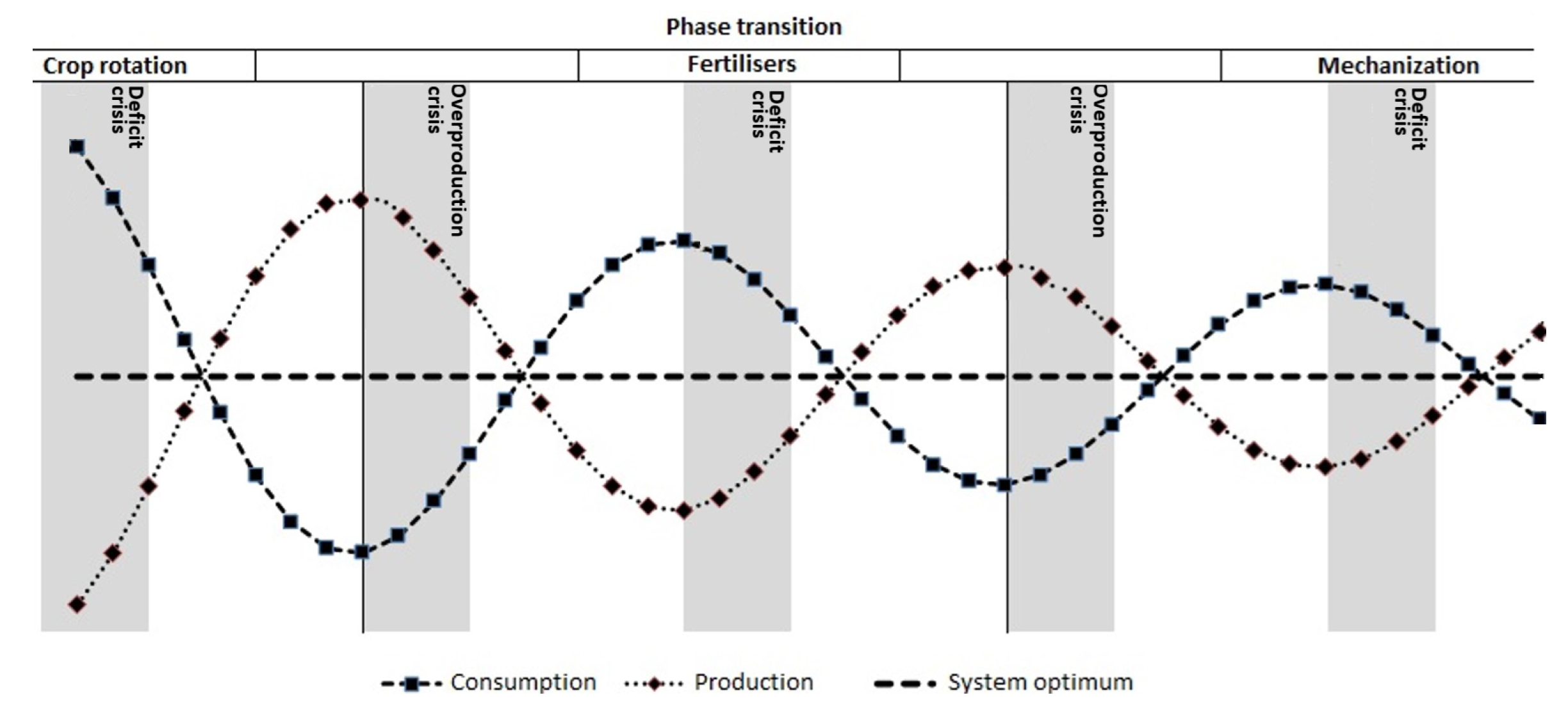
Such a system is adaptive. The adaptivity of the system in this respect is aimed at correcting the internal energy imbalance and achieving the state of optimum entropy. The system can be considered in terms of two counterpolar factors. The amplitude ratio and frequency response of such a system will then depend solely on the initial store of energy and the interference degree of the counterpolar parameters. Figure 1 shows an example of such a system in dynamics that are based on a case of agricultural production.

The simplest mathematical description of such a system is Equation (1):

$$f_n\left(t\right)\cong -f_{n+1}\left(t\right)\cong \phi \left(t\right)·\frac{A}{2},$$

(1)

where $f_n$ and $f_{n+1}$ are the counterdirectional factors (the sum of the interaction of which tends to result in the optimum entropy in time); A is the total energy expended on the interaction; and $\phi \left(t\right)$ is the periodic function.

In the process, both the supply of external energy and the adaptation of the system can lead to a change in amplitudes, phases, and frequencies $\phi \left(x\right)$. However, the main tendency of the aggregate system energy to a minimum remains unchanged. In this case, any energy supply into the system from the outside can be only presented as the amplitude variation of one of the system components with a simultaneous displacement of optimum entropy.

From a systemic point of view, the above model undergoes the phases of convergence and divergence. The boundaries of the transitions from a state of convergence to a state of divergence can be considered a crisis (from the Greek $\kappa \rho \iota \sigma \iota \varsigma$, which means turning point). The general definition of crisis implies that the beginning of this process corresponds to the extremum points at which the derivative of the first order $\phi \left(x\right)$ equals zero. According to I. R. Prigogine, phase transitions of the system are inevitable.

Given the fact that the economy is an open system, we can formulate a conclusion about the possibility of changes in the optimum entropy, phase, amplitude, and frequency of counterpolar factors in view of the inevitability of systemic crises (phase transitions). An example of an emerging systemic crisis can be found in the upcoming crisis of the world monetary system, a coming crisis that will be associated with the status transition of money from a substitute for exchange to a substitute for trust. This example is presented in Figure 2.

The above graph shows the criteria of the monetary system, such as the security, convenience, and criminality of money over the last three thousand years; these criteria are expressed on the normalized, ranking and evaluative scale that was designed by the authors based on historical data. As such, the convenience of use was evaluated in terms of the protective and accumulative properties of money. Criminality was assessed by the number of economic crimes that are possible with this type of money, and it was reflected in the remaining legislative sources. The security of money was estimated as a factor of guaranteed liquidity, and this was determined with regard to the source of guarantee and its possibilities.

The graph shows a reduction in the liquidity of currencies, while criminality and convenience of use are increasing. Thus, we observe a continuously growing gap between the security of money and its degree of criminality—in other words, a divergence of the monetary system that will sooner or later lead to a global crisis.

The crisis trends were found to be most pronounced in the financial sector of the economy, where the frequency of overheating and stock market crashes was particularly high.

Results of World Economic System Development

Starting from the middle of the last century, intensification processes have occurred in the economy. These process have entailed the development of data transmission facilities, an increase in transmission speed, as well as the enhancement of frequency and the velocity of transactions, thus leading to an overall economic advancement that has been achieved to the point of its overheating. Figure 3 and Figure 4 show summary diagrams of the economic crises that we know about from over the past 800 years.

Electronic trading, which has existed since 1867, has contributed to the expansion in the number and velocity of transactions in the financial market. Meanwhile, the nine orders of magnitude gain that we have seen over 145 years in the intensity and rate of data exchange (Figure 5) has been determined as being a fundamental factor in the increase in average economic crises frequency (Figure 6).

Based on the facts described above, there is a need to create an econometric model of crises.

In the first stage, we introduce the concept of an asset crisis indicator.

3. Asset Crisis Indicator

This paper presents the authors’ explanation of a crisis seen from the perspective of the ratio of market demand and supply with interchanging states of stability and imbalance. This series of states has definite stages of decline, plateau, and growth, as well as intermediate reversal states that also feature equilibrium and bifurcation points. As opposed to conventional models, where crises are often considered as a non-recurrent state (for instance, K. Marx’s market saturation point or P. Krugman’s bifurcation point), the authors of this paper choose to analyze it as an ongoing process. Based on statistical indicators, we propose a classification of the major crisis stages. We also develop a methodology through which to identify a crisis at its early stage, where it is detectable as a statistically unpredictable state that causes such a change in the indicator that it violates the valid bound constraints.

Thus, we argue that a crisis should be viewed not as a spontaneous and abrupt failure, but, contrarily, as a natural characteristic of the economy; one that has a particular development pattern.

However, after a crisis has started, it is possible to register its initial stage. This means that the next stages of the crisis may be projected accordingly.

The biggest problem in making managerial decisions is ignorance and incompleteness of information regarding the current situation as it develops. The ability to anticipate further developments is the most important factor when making managerial decisions. Therefore, the main task of this study was to create a model based on which it is possible not only to detect the beginning of the crisis process, but to also anticipate its further development and end. Solving this problem will bring practical benefits to managers at all levels, thereby helping them to make management decisions in a timely manner and to mitigate the consequences of crisis processes.

According to standard statistical representations, the short-term standard deviation of random fluctuations with a probability of 99.72% cannot exceed the standard deviation that is accumulated over the previous period by more than three times (i.e., the three-sigma rule). However, when analyzing the value of exchange-traded assets, it turns out that not only do such phenomena exist, but that they are also the main cause of unexpected loss or profit. These phenomena can be regarded as sudden, unpredictable changes in the system of assets that make up an investment portfolio. In other words, as crises of individual assets. To avoid unforeseen losses, such asset states should be monitored and evaluated in the eventual need that the portfolio is re-optimized (rebalanced).

According to the results of the below experiment, which analyzed the prices of 620 exchange-traded assets in the period of 1 January 1980 to 1 June 2016, 710 states of asset crises were detected and analyzed. The main identified features included the following:

• The invariance of asset crises allowed for identifying the phases of the crisis process and modeling changes in the standard deviation of the price fluctuations of a normalized time series during a crisis period;
• The mode value of the ratio of short-term and long-term standard deviations was equal to 2.99, which confirmed the hypothesis of the normality of the distribution of market noise and compliance with the three-sigma rule in non-crisis periods.

Let us assume that, to determine the presence of a crisis, the main method will be to check the short-term standard deviation of the asset price for compliance with the “three-sigma rule”, as shown in Formula (2):

$$\left(\frac{{\sigma }_{\tau }}{{\sigma }_t}>3\right)$$

(2)

In this case, the variances of the short-term and long-term samples were compared, and they were found to be similar according to a Fisher statistical test [39], as shown in Formula (3):

$$F_F=\frac{{\widehat{\sigma }}_X^2}{{\widehat{\sigma }}_Y^2}\sim F(m-1;n-1),$$

(3)

where $F_F$ is Fisher’s test statistic; ${\widehat{\sigma }}_{X,Y}^2$ are the unbiased sample variances; and $m,n$ is the number of sample units.

Since the boundary of the crisis criterion was clearly defined as three sigmas—and as both samples belong to the same normalized general population—it is possible to modify the criterion to a more simplified form with a unit boundary and standard deviation instead of variance, as is shown in Formula (4):

$$C_F=3{\sigma }_{\tau }-{\sigma }_t,$$

(4)

where $C_F$ is the modified Fisher’s test with a unit boundary; ${\sigma }_{\tau }$ is the short-term standard deviation; and ${\sigma }_t$ is the accumulated standard deviation.

To apply $C_F$ as an indication of the presence of a crisis, we used the Heaviside function with a simultaneous reduction in $C_F$ to the interval that has a zero boundary corresponding to ${\sigma }_t$, as is shown in the Formula (5):

$$C=H(C_F-{\sigma }_t)$$

(5)

Or as is shown in Formulas (6) and (7):

$$C=H(3{\sigma }_{\tau }-2{\sigma }_t)$$

(6)

$$C_0=H(2{\sigma }_t-3{\sigma }_{\tau }),$$

(7)

where C is the indication of the presence of a crisis; $C_0$ is the indication of the absence of a crisis; H is the Heaviside function; ${\sigma }_{\tau }$ is the standard deviation of price fluctuations for the analytical period; and ${\sigma }_t$ is the accumulated standard deviation.

This modified Fisher’s test will be referred to as a crisis indicator. This indicator has only two values (which are shown in

Table 1. Values of the crisis indicator function.

Presence of a Crisis	Function Value $\mathit{C}=\mathit{H}(3{\mathit{\sigma }}_{\mathit{\tau }}-2{\mathit{\sigma }}_{\mathit{t}})$	Function Value ${\mathit{C}}_0=\mathit{H}(2{\mathit{\sigma }}_{\mathit{t}}-3{\mathit{\sigma }}_{\mathit{\tau }})$
No	0	1
Yes	1	0

and are convenient to use for generating IF-THEN functions): 1 and 0.

The intensity of the crisis processes may be different for different assets. The relative intensity indicator may reflect the severity of a given crisis. The ratio of the short-term exceedance of a crisis boundary to its height is quite significant, as shown in Formula (8):

$$(3{\sigma }_{\tau }-2{\sigma }_t)/{\sigma }_t$$

(8)

Combining this indicator with the crisis indicator, we obtain a value that characterizes the intensity of the crisis in accordance with

Table 2. Values of the crisis intensity function.

Presence of a Crisis	Function Value I
No	0
Yes	$(0;+\infty )$

, as shown in Formula (9):

$$I=C\frac{(3{\sigma }_{\tau }-2{\sigma }_t)}{{\sigma }_t},$$

(9)

where I is the intensity of the crisis; $C=H(3{\sigma }_{\tau }-2{\sigma }_t)$; H is the Heaviside function; ${\sigma }_{\tau }$ is the standard deviation of price fluctuations for the analytical period; and ${\sigma }_t$ is the accumulated standard deviation.

In fact, the intensity indicator I reflects the z-statistics of the short-term deviation that exceeds the accumulated values of asset price fluctuations, thus showing the probability of a crisis for the current state of the asset.

4. Crisis Risk

In the second stage, we introduce the concept of crisis risk. The crisis risk of changes in the asset price is calculated based on a mathematical phase model of the asset crisis, which was obtained as the result of a statistical experiment described below.

According to this model (Figure 7), for the values $\Delta {\sigma }_{\underline{t}}$ that are normalized by ${\sigma }_{\max }$ and which are in the crisis period normalized by its duration t, there is an excess $\Delta {\sigma }_{\underline{t}}$ of the short-term standard deviation ${\sigma }_{\underline{t}}$ of the asset above the level $3{\sigma }_{\underline{t}}$. This corresponds to Formula (10):

$$\Delta {\sigma }_{\underline{t}}\left(t\right)=0.989{(sin\pi t)}^{2.543}\pm 0.254{|sin2\pi t|}^{1.135},$$

(10)

where $\Delta {\sigma }_{\underline{t}}\left(t\right)$ is the normalized increment of the short-term deviation ${\sigma }_{\underline{t}}$ during the crisis at time t.

Accordingly, the upper bound of the risk increment model was calculated using Formula (11):

$${\sigma }_{sup}\left(t\right)=\Delta {\sigma }_{max}=\left(0.989{\left(sin\pi \frac{t_s}{\overline{t_c}}\right)}^{2.543}+0.254{\left|sin2\pi \frac{t_s}{\overline{t_c}}\right|}^{1.135}\right),$$

(11)

where ${\sigma }_{sup}\left(t\right)$ is the supremum of the increment of the crisis risk at moment t; $t_s$ is the time frame from the onset of the asset crisis; and $\overline{t_c}$ is the mean duration of crises for the given asset.

Thus, the risk of a crisis decline in the asset price is calculated according to Formula (12):

$$R_C=C·\left({\sigma }_t·\frac{{\sum }_{i=1}^k\frac{{\sigma }_{{\tau }_{C_i}}}{i^{a_h}}}{{\sum }_{i=1}^k\frac{1}{i^{a_h}}}·\left(0.989{\left(sin\pi \frac{t_s}{t_c}\right)}^{2.543}+0.254{\left|sin2\pi \frac{t_s}{t_c}\right|}^{1.135}\right)\right),$$

(12)

where C indicates the existence of an asset crisis; ${\sigma }_{\tau }$ is the non-crisis SD of T; ${\sigma }_{{\tau }_{C_i}}$ is the highest SD in the course of the i-th crisis; $t_s$ is the time frame from the onset of the asset crisis; $\overline{t_c}$ is the mean duration of the crises of a given asset; k is the quantity of asset crises that took place in the past; and $a_h$ is Holt’s data decay coefficient.

5. Development of an Econometric Model of the Asset Crisis

To arrange the sequence of experiments and generalize the results obtained, we will draw up a plan of the experimental part for the purposes of formalizing and verifying the econometric model of the crisis.

Plan for the experiment.

Objective: To test the main economic hypotheses.

Method: Statistical analysis of real data.

Experiments:

• Feasibility check of the hypothesis regarding individual asset crises, as well as a definition of the values of the crisis criterion used in the model;
• Feasibility check of the hypothesis regarding the time boundedness of a crisis and its distribution;

  -

  Check the hypothesis regarding crisis duration distribution;

• Feasibility check of the hypothesis regarding the invariance of crises, as well as the phase estimates used in the model;
• Construction of a phase statistical model of the Moscow Exchange asset crisis;
• Test of the phase statistical model of the Moscow Exchange asset crisis;
• Assessment of the quality of the empirical data approximation based on the phase model of the Moscow Exchange asset crisis.

A stratification of the Russian investment assets market is performed, as shown in

Table 3. Stratification of the investment asset market.

Stratification of Investment Assets for Statistical Sampling
		Life Period in the Market
		7 Years or More	3–6 Years	Less Than Three Years
Rate of return over the life period	Significant positive	1	2	3
	Insignificant	2	3	4
	Significant negative	3	4	5

. As the main stratified sample for the study, the assets from stratum No. 1 were taken. To achieve the required sample size, statistical data on the value of strategic investment assets in the world and Russian markets were collected. The initial data for the experiments was the time series of the daily closing prices of 620 assets, where at least 7 years was monitored for each. The total sample size was at least 1,000,000 units. Of these, we had the following: 131 Russian assets and 489 foreign assets.

5.1. Feasibility Check of the Hypothesis Regarding an Individual Asset Crisis, as Well as a Definition of the Values of the Crisis Criterion Used in the Model

The economic rationale of the experiment was as follows: in taking, as a starting point, the axiom of market homogeneity (the axiom of ergodicity) [40], we must accept, as the main property of ergodicity, the repetition of macroeconomic processes (global crises) at the microeconomic level (crises of individual assets). Let us check this statement.

The purpose of the experiment was to test the feasibility of the market state model.

The asset market state evaluation model consisted of five statements, with three statements describing the states such as “growth”, “stagnation”, and “decline” (which do not require a statistical check since their statistical significance corresponds to $\alpha =0$, i.e., it is trivial). At the same time, the statements about “crisis growth” and “crisis decline” required a feasibility check.

Each statement consists of a trivial part and a feasible part:

• “crisis growth” = “crisis”; $\alpha =x+$ “growth”; $\alpha =0$;
• “crisis decline” = “crisis”; $\alpha =x+$ “decline”; $\alpha =0$.

Let us check the feasibility of the concept of “crisis” with $\alpha =0.05$.

The representativeness of the world’s top 500 financial companies was set according to the Bloomberg index and 131 assets of the Russian MICEX market.

The sample test was of the strategic investment potential (≥7 years).

The sample units were the ratios of a short-term and the cumulative standard deviations averaged over the asset series ${\sigma }_{\tau }/{\sigma }_t$.

$H_1$—the average ratio of the cumulative variability of the asset to the short-term variability obeys a certain law of distribution.

$H_0$—distribution regularities of the average ratio of the cumulative variability of the asset to the short-term variability do not exist.

Rejection tests: test ${\chi }^2$ and Student’s t-test.

Experimental conditions: N—general population; n—sample size; ${}_{min}$—the minimum required sample size for $\alpha =0.05$; $d{f}_{St}$—the number of degrees of freedom according to Sturges’ rule; and $d{f}_{\alpha }$—the number of degrees of freedom for alpha grouping.

• $N>10,000;n=620;\alpha =0.05;n_{min}=384;d{f}_{St}=8;d{f}_{\alpha }=19$;
• $H_0:$ Test ${\chi }_{St}^2\le 0.75$;
• $H_0:$ Test ${\chi }_{\alpha }^2\le 0.95$ v t-test $\le 0.95$;
• $H_1\leftrightarrow \neg H_0$.

Let us perform the grouping with Sturges’ rule [41].

Figure 8 shows the construction of a Sturges histogram.

Let us perform the $\alpha$-grouping. Figure 9 shows the construction of an $\alpha$-histogram.

When considering the histograms, no evidence against the postulated trends was found. $H_0$ was not confirmed intuitively.

We thus carried out a criterion estimation by means of the Sturges Chi-square test for a standard normal distribution:

$$\mathrm{Test}{\chi }_{St}^2=0.763;0.763>0.75\to >H_0$$

Given the low power of the ${\chi }_{St}^2$ criterion, we used the more powerful Test ${\chi }_{\alpha }^2$ and t-test for a biased normal distribution. Figure 10 shows a graphical representation of the t-test for a biased normal distribution.

$$\mathrm{Test}{\chi }_{\alpha }^2=0.969;t\mathrm{-test}=0.994;0.994>0.969>0.95\to \neg H_0$$

The rejection $H_0$ was obtained; thus, we accept $H_1$.

If $H_1$ is accepted, it is necessary to establish the reason for the bias of the distribution to the right. It is because of exchange rules and regulations that asset trading with price fluctuations $\approx 4{\sigma }_t$ is halted on most exchanges till the stabilization of the market situation.

Preliminary conclusion: Since $H_1$ is accepted and the reasons for the bias established, we allowed the definition of “crisis” to also include the exceedance of the relation ${\sigma }_{\tau }/{\sigma }_t$ over a certain measure of the central tendency of a standard deviation.

To determine the range of values of the crisis criterion, we conducted a statistical study on the historical values of the ratio of the short-term standard deviation to the cumulative one.

Table 4. Descriptive sample statistics rounded to hundredths.

Average	3.14
Median	3.15
Mode	2.99
Minimum	2.06
Maximum	4.0
Interval	1.94
Sample variance	0.11
Standard deviation	0.33
Standard error	0.01
Kurtosis	0.59
Skewness	−0.35

provides descriptive sampling statistics of the ratio of short-term and cumulative variability ${\sigma }_{\tau }/{\sigma }_t$ for 620 assets over 7 years (more than 1,000,000 sample units) to determine the boundary of the “crisis” state.

Using the principle of lowest risk preference, we determined the boundary of the crisis state as the smallest measure of central tendency (MCT) of the ratio of the standard deviations.

Since $3.15>3.14>2.99$, such is the mode of distribution, thus coarsening the measure to an integer number of z-values. Therefore, the attribute of “crisis” can be described as $H(3{\sigma }_{\tau }-{\sigma }_t)$.

Conclusions

The expression of the form $H(3{\sigma }_{\tau }-{\sigma }_t)$ is statistically significant, and it is a representative of the presence of a “crisis” of the asset.

For an intuitive assessment and for hypothesizing, we constructed graphs of the values of the crisis variability ${\sigma }_{tC}$ that were normalized by a maximum of 20 randomly selected asset crises, as shown in with Figure 11.

Let us formulate a number of intuitive hypotheses describing the variance of the exchange-traded assets in times of crisis:

• Crises are bounded by time;
• The duration of crises has general tendencies;
• During their development, crises have at least two phase states.

5.2. Check of the Hypothesis Regarding a Crisis’ Time Boundedness

The economic rationale of the experiment: A crisis can not be endless, sooner or later the market returns to a stable state. Let us check this statement.

5.2.1. The Experiment Objective

To verify the hypothesis regarding the limited duration of the asset crisis defined in Section 5.1, we performed the following:

• The representativeness was a random sample of MICEX assets;
• The sample test was on the short-term strategic investment potential (≥5 years);
• The sample units were the days of the asset crises’ duration;
• $H_1$—the duration of most crises of MICEX strategic assets is bounded to a certain time period;
• $H_0$—the duration of most crises of MICEX strategic assets is not bounded by time;
• The dismissal test was the binomial m-test;
• $N>10,000;n=710;\alpha =0.05;n_{min}=384;d{f}_{Bin}=1$;
• $H_0:m\le 0.95$;
• $H_1\leftrightarrow \neg H_0$.

Let us perform a binomial grouping. Figure 12 shows a binomial histogram.

In the present histogram, the postulated trends were detected, and $H_0$ was not confirmed intuitively.

We carried out the estimation by means of the binomial m-test:

$m=0.956;0.956>0.95\to \neg H_0$.

The rejection of $H_0$ was obtained; thus, we accept $H_1$.

5.2.2. Conclusions

The duration of most of the crises of the MICEX strategic assets was bounded to a period of 35 days with $\alpha <0.05$.

5.3. Check of the Hypothesis of the Crisis Duration Distribution

The economic rationale of the experiment: Since the duration of the crisis was limited, it may obey some of the laws of distribution. Let us check this statement.

5.3.1. The Purpose of the Experiment

We tested the hypothesis that the duration of the asset crisis obeys a certain law of distribution.

The sample was a random sample of the assets of the Moscow Exchange. The hypotheses regarding the distribution of the duration of crises of strategic assets of the Moscow Exchange were as follows:

• $H_0$ is antimodal;
• $H_1$ is unimodal;
• $H_2$ is bimodal;
• $H_3$ is polymodal;
• The rejection test was Hartigan’s Dip test [42];
• $N>10,000;n=710;\alpha =0.05;\alpha =0.01;n_{min}=384;d{f}_{max}=68$;
• $H_0:\alpha =0.05;DI{P}_1\le 0.037$;
• $H_1:\alpha =0.05;DI{P}_1\ge 0.037;DI{P}_2\le 0.037$;
• $H_2:\alpha =0.01;DI{P}_1\ge 0.0429;DI{P}_2\ge 0.0429;DI{P}_3\le 0.0429$;
• $H_3:\alpha =0.01;DI{P}_1\ge 0.0429;DI{P}_2\ge 0.0429;DI{P}_3\ge 0.0429$;
• $H_0\leftrightarrow \neg H_{1,2,3}$;
• $H_1\leftrightarrow \neg H_{0,2,3}$;
• $H_2\leftrightarrow \neg H_{0,1,3}$;
• $H_3\leftrightarrow \neg H_{0,1,2}$.

We then performed a grouping with $d{f}_{max}$.

Let us construct the histogram. First, we should perform a DIP-test. Figure 13 shows the results from Hartigan’s Dip test for modality.

$$DI{P}_1=0.04367;DI{P}_2=0.04346;DI{P}_3=0.04113$$

$$DI{P}_1\ge 0.0429;DI{P}_2\ge 0.0429;DI{P}_3\le 0.0429\to \neg H_{0,1,3}\to H_2$$

We accepted that $H_2$ is a bimodal distribution with $\alpha =0.01$.

Let us describe the statistics for a bimodal normal distribution. Figure 14 shows the distribution of the duration of the crises.

$${\mu }_1=0.0575;{\mu }_2=0.3437;{\sigma }_1=0.1055;{\sigma }_2=0.1005;\Delta y=0.0428$$

Let us test ${\chi }^2$ and Student’s t-test for this distribution:

$$\mathrm{Test-}{\chi }^2=0.7656;t\mathrm{-test}=0.9296$$

5.3.2. Conclusion

The bimodal normal distribution describes the normalized duration of the asset crises, with $\alpha$ being at least 0.25, via the statistics of the following form (

Table 5. Statistics on the duration of asset crises.

Median, mode, mean ${\mathit{\mu }}_1$	0.0575
Median, mode, mean ${\mu }_1$	0.3437
Standard deviation ${\sigma }_1$	0.1055
Standard deviation ${\sigma }_2$	0.1005
Bias of distribution $\Delta y$	0.0428
Ashman’s D (amplitude of antimode)	0.8919
Shilling’s-S (similarity of distributions)	0.9988

):

Thus, the following day’s values can be taken as the respective median values of the duration of crises:

$$t_{c_1}=\lfloor {\mu }_1·t_{c_{max}}\rfloor =\lfloor 0.0575·69\rfloor =4\mathrm{days}(\mathrm{for}\mathrm{short-term}\mathrm{crises});$$

$$t_{c_2}=\lfloor {\mu }_2·t_{c_{max}}\rfloor =\lfloor 0.3437·69\rfloor =24\mathrm{days}(\mathrm{for}\mathrm{long-term}\mathrm{crises}).$$

5.4. Check of the Hypothesis Regarding Crisis Invariance

The economic rationale of the experiment: Since the duration of the crisis was limited, and as it obeyed a certain law of distribution, the dynamics of the development of all crises were found to be similar and consisted of several phases. Let us check this statement.

5.4.1. The Experiment Objective

The aim it to verify the hypothesis regarding the existence of phases of crisis variability changes and their identity.

The sample was a random sample of 98 out of a 710 time series of relative values of the standard deviation of assets in crisis periods, and these were normalized by the duration of the crises.

The hypotheses regarding the phases of the crisis variability changes were as follows:

• $H_0$ does not exist;
• $H_1$ do exist, but they are specific for each crisis;
• $H_2$ does exist and obeys a certain law of distribution;
• The test-${\chi }^2$ test was the rejection test;
• $N>10,000;n=98;\alpha =0.05;n_{min}=96$;
• $H_0:\alpha =0.05;sgn\overline{{\sigma }_{{\tau }_C}^{\prime }}\left(t\right)=sgn\overline{{\sigma }_{{\tau }_C}^{\prime }}(\forall t)$,
• where ${\sigma }_{{\tau }_C}$ is the standard deviation during the crisis;
• $\overline{{\sigma }_{{\tau }_C}^{\prime }}(\forall t)$ is the sample mean of the standard deviation;
• $H_1:sgn{\sigma }_{\sigma }^{\prime }\left(t\right)=sgn{\sigma }_{\sigma }^{\prime }(\forall t);sgn\overline{{\sigma }_{{\tau }_C}^{\prime }}\left(t\right)\ne sgn\overline{{\sigma }_{{\tau }_C}^{\prime }}(\forall t)$;
• $\overline{{\chi }^2}\ge P_{\alpha }$,
• where ${\sigma }_{\sigma }\left(t\right)$ is the standard deviation from the sample mean;
• $H_2:sgn{\sigma }_{\sigma }^{\prime }\left(t\right)\ne sgn{\sigma }_{\sigma }^{\prime }(\forall t);sgn\overline{{\sigma }_{{\tau }_C}^{\prime }}\left(t\right)\ne sgn\overline{{\sigma }_{{\tau }_C}^{\prime }}(\forall t);{\chi }^2\ge P_{\alpha }$;
• $H_0\leftrightarrow \neg H_{1,2}$;
• $H_1\leftrightarrow \neg H_{0,2}$;
• $H_2\leftrightarrow \neg H_{0,1}$.

We shall now consider the mean-value and standard-crisis-variability-deviation piecewise linear functions that were normalized by ${\sigma }_{{\tau }_C}$ and ${\sigma }_{\sigma }$, as shown in Formulas (13) and (14).

$$\overline{{\sigma }_{{\tau }_C}}\left(t\right)=\overline{\left({\sigma }_{{\tau }_C}\left(t\right)-{\sigma }_t\left(t\right)\right)}$$

(13)

$${\sigma }_{\sigma }\left(t\right)=\sqrt{D\left[{\sigma }_{{\tau }_C}\left(t\right)\right]}$$

(14)

$${\sigma }_{{\tau }_C}\left(t\right)\in [0;1];{\sigma }_{\sigma }\left(t\right)\in [0;1]$$

Let us construct and consider the complete histogram for $\overline{{\sigma }_{{\tau }_C}}\left(t\right)$ and ${\sigma }_{\sigma }\left(t\right)$.

Figure 15 shows the graphs of the crisis variability.

In the present histogram, the postulated trends were detected, and $H_0$ was not confirmed intuitively.

We next calculated the derivative values $\overline{{\sigma }_{{\tau }_C}}\left(t\right)$.

$$\overline{{\chi }^2}=0.999;sgn\overline{{\sigma }_{{\tau }_C}^{\prime }}\left(t\right)\ne sgn\overline{{\sigma }_{{\tau }_C}^{\prime }}(\forall t)$$

$${\chi }^2>0.95;\overline{{\sigma }_{{\tau }_C}}\left(t\right)\ne \overline{{\sigma }_{{\tau }_C}}(\forall t);\to \neg H_0$$

Then, the rejection of $H_0$ happened.

We next calculated the derivative values $\overline{{\sigma }_{{\tau }_C}^{\prime }}\left(t\right)$ and ${\sigma }_{\sigma }^{\prime }\left(t\right)$. We then constructed and considered a normalized cumulative histogram of derivative signs $sgn\overline{{\sigma }_{{\tau }_C}^{\prime }}\left(t\right)$ and $sgn{\sigma }_{\sigma }^{\prime }\left(t\right)$, which are presented in Figure 16.

In the present histogram, the postulated trends were detected, and $H_1$ was not confirmed intuitively.

$${\chi }^2=0.999;sgn{\sigma }_{\sigma }^{\prime }\left(t\right)\ne sgn{\sigma }_{\sigma }^{\prime }(\forall t);$$

$$\overline{{\chi }^2}>0.95;sgn{\sigma }_{\sigma }^{\prime }\left(t\right)\ne sgn{\sigma }_{\sigma }^{\prime }(\forall t)\to \neg H_1;$$

Then, the rejection of $H_1$ happened.

If $\neg H_0$, $\neg H_1\to H_2$, then we accept $H_2$.

5.4.2. Conclusion

The phases of the asset crises variability changes exist and obey a certain law of distribution.

5.5. Construction of a Phase Model of the Crisis

The economic rationale of the experiment: Since the duration of the crisis was limited and obeyed a certain distribution law—and as the dynamics of the development of all crises were found to be similar and consisted of several phases—it was possible to create an approximation model that allowed for predicting both the duration and the risk component in crisis periods. Let us check this statement.

5.5.1. The Purpose of the Experiment

To create a statistically significant phase model of the crisis of the Moscow Exchange asset, as is defined in Section 5.3.

To build the model, we used a sample of 98 maximum-aligned time series of asset variability values in crisis periods that were normalized by value and time with an acceptable error not exceeding 0.025, thus corresponding to $\alpha /2$ for $\alpha =0.05$.

When analyzing the model, the main formative factors were the average normalized value of the crisis variability $\overline{{\sigma }_{{\tau }_C}^{\prime }}\left(t\right)$ that corresponded to the value $\overline{\left(3{\sigma }_{{\tau }_C}\left(t\right)-{\sigma }_t\left(t\right)\right)}$ and the mean proper standard deviation of the time series variability $\overline{{\sigma }_{\sigma }}$. Figure 17 shows the normalized input data for the model generation.

Let us assume that, for the construction of a reference function of the form ${\sigma }_H\left(t\right)\pm {\sigma }_{{\sigma }_H}$ in the case of unbiased phases, the following phase correspondence will be true, as shown in Formula (15):

$$\phi \left({\sigma }_{{\tau }_C}\left(t\right)\right)\widehat{=}\pi ;\phi \left({\sigma }_{\sigma }\right)\widehat{=}2\pi$$

(15)

We represent ${\sigma }_{{\tau }_C}$ and ${\sigma }_{\sigma }$ in the form of periodic functions, as shown in Formula (16):

$${\sigma }_{{\tau }_C}\left(t\right)=a_1·{(sin\pi t)}^{b_1};{\sigma }_{\sigma }=a_2{|sin2\pi t|}^{b_2}$$

(16)

When using the generalized reduced gradient method, we approximated the smoothed moving average values of ${\sigma }_{{\tau }_C}\left(t\right)$ and ${\sigma }_{\sigma }\left(t\right)$ by the functions of the form $a_1{(sin\pi t)}^{b_1}$ and $a_2{|sin2\pi t|}^{b_2}$, respectively. Figure 18 shows the approximation of the smoothed averages by periodic functions.

The results of the approximation are presented as according to Formula (17).

$$a_1=0.989;b_1=2.543;{\phi }_1=\pi ;a_2=0.254;b_2=1.135;{\phi }_2=2\pi ;$$

$${\sigma }_{{\tau }_C}\left(t\right)=0.989{(sin\pi t)}^{2.543}\pm 0.254{|sin2\pi t|}^{1.135}\mathrm{for}t\in [0;1]$$

(17)

Figure 19 shows the range of acceptable values ${\sigma }_{{\tau }_C}\left(t\right)$ of the model for deviation ${\sigma }_{\sigma }\left(t\right)$.

Having identified ${\sigma }_{{\tau }_C}^{\prime }\left(t\right)$ and ${\sigma }_{{\tau }_C}^{\prime \prime }\left(t\right)$, let us describe the main points and phases of the model of the crisis development of the Moscow Exchange strategic asset, as shown in Formulas (18) and (19):

$${\sigma }_{{\tau }_C}^{\prime }\left(t\right)=0.989\left(2.543{(sin\pi t)}^{1.543}cos\pi t\right)$$

(18)

$${\sigma }_{{\tau }_C}^{\prime \prime }\left(t\right)=0.989\left(2.543\left(1.543{(sin\pi t)}^{0.543}cos\pi t\right)cos\pi t-2.543{(sin\pi t)}^{1.543}sin\pi t\right)$$

(19)

Figure 20 shows the values of the derivatives of ${\sigma }_{{\tau }_C}$.

Table 6. Development phases of the Moscow Exchange strategic asset crisis.

Type	Title	${\mathit{\sigma }}_{{\mathit{\tau }}_{\mathit{C}}}\left(\mathit{t}\right)$	${\mathit{\sigma }}_{{\mathit{\tau }}_{\mathit{C}}}^{\prime }\left(\mathit{t}\right)$	${\mathit{\sigma }}_{{\mathit{\tau }}_{\mathit{C}}}^{\prime \prime }\left(\mathit{t}\right)$	t
Point	Of the crisis’ beginning	≈0	>0	>0	≈0
Phase	Of the growth acceleration	$(0;1)$			$(0;0.3)$
Point	Of changes in dynamics			≈0	≈0.3
Phase	Of the growth declining			$<0$	$(0.3;0.5)$
Point	Of the crisis plateau	≈1	≈0		$\approx 0.5$
Phase	Of the decline acceleration	$(0;1)$	$<0$		$(0.5;0.7)$
Point	Of changes in dynamics			≈0	≈0.7
Phase	Of the slowdown in the decline			$>0$	$(0.7;1)$
Point	Of the crisis’ end	≈0			≈1

shows the development phases of the crisis of the Moscow Exchange strategic asset.

5.5.2. Conclusions

A phase model of the development of the crisis of the Moscow Exchange strategic asset was created. Since the creation of the model is based on a non-obvious statement about the correspondence of the form $\phi \left({\sigma }_{{\tau }_C}\right)\widehat{=}\pi ;$$\phi \left({\sigma }_{\sigma }\right)\widehat{=}2\pi$, the model performance should be evaluated analytically for a given $\alpha =0.05$.

5.6. Test of the Phase Model of the Asset Crisis

The economic rationale of the experiment: The approximate phase model of the crisis allows for the predicting of the risk components in crisis periods. Let us test this statement on the empirical data.

5.6.1. The Purpose of the Experiment

The aim was to check the quality of the created phase model of the crisis variability of the Moscow Exchange asset.

• The representativeness covered a random sample of short-term standard deviation values in the crisis periods of 31 strategic investment assets of the MICEX;
• The sample units were the 7154 normalized values of the variability exceedance $(3{\sigma }_{{\tau }_C}-{\sigma }_t)$ of the crisis time series that was normalized by the duration of the crises of the MICEX assets, which was also normalized by the maximum standard deviation;
• $H_0$—the quality of the phase model of the crisis was not statistically confirmed;
• $H_1$—the quality of the phase model of the crisis was sufficient for $\alpha =0.05$;
• The rejection test was the binomial m-test;
• The applicability test of the dismissal test was the accurate binomial test;
• $N>10,000;n=7154;\alpha =0.05;n_{min}=384;d{f}_{Bin}=1$;
• $H_0:m_{2\sigma }<1-\alpha ;P_{value}\ge \alpha$;
• $H_1\leftrightarrow \neg H_0$.

Let’s perform a binomial grouping by consider it in a histogram. Figure 21 shows the testing of the model.

In the present histogram, the postulated trends were detected, and $H_0$ was not confirmed intuitively.

We shall carry out the estimation by means of the binomial m-test:

$$m_{2\sigma }=0.957;P_{value}=0.000319;m_{2\sigma }>1-\alpha \wedge P_{value}\ll \alpha \to \neg H_0$$

The rejection of $H_0$ was obtained; thus, we accept $H_1$.

5.6.2. Conclusions

According to the statistical evaluation, the created phase model of the crisis development of the MICEX strategic asset sufficiently met the requirements of the model quality for a given $\alpha =0.05$.

5.7. Evaluation of the Quality of the Approximation of Empirical Data Based on the Phase Model of the Moscow Exchange Asset Crisis

The economic rationale of the experiment: The approximate phase model of the crisis allows for the predicting of the duration of a crisis in crisis periods. Let us test this statement on the empirical data.

5.7.1. The Purpose of the Experiment

The aim was to check the adequacy of the approximation quality of the phase model of the crisis variability during the calculation of the model coefficients.

The representativeness was a sample of the residual, as shown in Formula (20):

$$\epsilon ={\sigma }_{{\tau }_{C_E}}\left(t\right)-{\sigma }_{{\tau }_{C_M}}\left(t\right),$$

(20)

where ${\sigma }_{{\tau }_{C_E}}\left(t\right)$ is obtained empirically; ${\sigma }_{{\tau }_{C_M}}\left(t\right)$ is modeled based on the values of a random sample of the 7054 values of the crisis variability of the Moscow Exchange assets.

• $H_0$—the residuals were homoscedastic and stationary;
• $H_1$—the residues were not homoscedastic and not stationary;
• The rejection tests used were the White test and F-test;
• $N>10,000;n=7055;\alpha =0.05;n_{min}=384;df=7054$;
• $H_1;F>F_{\alpha };\vee LM<{\chi }_{\alpha }^2$;
• $\neg H_1\leftrightarrow H_0$,

where F is Fisher’s test; $F_{\alpha }$ is the table value for $\alpha$; $LM$ is the Lagrange multiplier statistic; and ${\chi }_{\alpha }^2$ is the table value for $\alpha$.

Figure 22 shows a histogram of the residuals.

When considering the histogram, the similarity with the Bessel distribution was revealed, and the postulated trends were detected. $H_0$ was not confirmed intuitively.

We then ran the White test and the F-test as follows:

$$F=26.41;F_{\alpha }=3.84;LM=1.67·{10}^{-11};{\chi }_{\alpha }^2=3.93·{10}^{-3}$$

$$F>F_{\alpha };\vee LM\ll {\chi }_{\alpha }^2;\to \neg H_1$$

It was then found that the rejection of $H_0$ did not happen.

Thus, the developed mathematical phase model of asset crisis was constructed with the help of a approximation approach that allows one to predict the development of crisis with an accuracy of $\alpha \le 0.05$, as well as helps with defining the dates of the beginning and end of asset crises. Figure 23 shows an example of a risk forecast on a EUR/RUB currency pair.

Figure 24 shows an example of a risk forecast on a EUR/RUB currency pair.

Figure 25 shows an example of a risk forecast on a EUR/RUB currency pair.

Based on the conducted research, it can be concluded that the tendencies to fluctuations in free prices in the stock exchange market have a distinct inclination to a normal distribution, one that is apart from the periods of crisis changes. At the same time, the movements in price during crisis periods are yet more proof of the importance of the three-sigma rule. However, in spite of that, the crisis fluctuations in prices across the market are also normally distributed. In asset crises, four identical phases were identified. These phases not only allowed for predicting possible crisis movements in prices, but they also allowed them to be made with acceptable accuracy after the second phase, which makes it possible to define the ending date of the crisis.

An analysis of a 533 time series when determining the capabilities of the crisis indicator and the range of its application was carried out. Figure 26, Figure 27 and Figure 28 show the graphs of assets with known crisis states.

5.7.2. Conclusions

We designed a crisis indicator and a crisis development model that exhibited an ample degree of generality, as well as a level of convincing fidelity regarding the properties aimed at detecting an economic crisis. The designed model was able to achieve a higher effectiveness when compared to the other models due to its validity and statistical capability in making both practical and theoretical predictions of the volatility.

An experiment was conducted to assess the quality of the econometric crisis model on real historical data. The results of the experiment showed the high quality of the model as a crisis detection tool. To identify the crisis phases, it was sufficient to approximate the crisis process by first-order derivatives.

In a statistical analysis of a 620 time series of transnational and Russian investment assets with strategic potential (which had existed for more than 7 years), the hypothesis of crisis invariance was not refuted as follows:

• In terms of the feasibility of the invariant crisis model with $\alpha =0.05$, there was a confirmation of the hypothesis regarding the invariance of crises;
• In terms of the invariance of the duration of crises with $\alpha =0.05$, there was a confirmation of the hypothesis regarding the duration of crises;
• In terms of the invariance of the crisis phases with $\alpha =0.05$, there was a confirmation of the hypothesis regarding the sequence of the crisis phases.

Thus, a method for determining asset crises was developed, and a phase model of the crisis was created.

6. Conclusions

Thus, through the implemented model, we conclude that the tendencies toward fluctuations in the free prices in the stock exchange market have a distinct inclination to a normal distribution, and this is apart from the periods of crisis changes. At the same time, the movements in price during crisis periods are yet more proof of the importance of the three-sigma rule; however, in spite of that, the crisis fluctuations in prices across the market were also found to be normally distributed. In asset crises, four identical phases were identified, which not only allowed for the predicting of possible crisis movements in prices, but they were also made with acceptable accuracy after the second phase, which enabled us to define the ending date of the crisis. As, primarily, an approximation model, the created phase model of crises allows for a determination of the duration of the crisis, after its first phase, with a sufficiently high probability. This also allows for defining its ending date during the second phase of the crisis with a substantial degree of probability. The result of the study was in establishing a functioning mathematical model for forecasting asset risks in times of crisis. As for possible limitations of the current model and thus possible extensions for taking the model further (as well as future research topics), we would like to point out once again that the developed mathematical model of crises was primarily designed to identify and predict the end of asset crises (such as crude oil, gold, stocks, currency pairs, and other tradable assets).