Ensemble Learning for Multi-Label Classification with Unbalanced Classes: A Case Study of a Curing Oven in Glass Wool Production

Abstract

The Industrial Internet of Things (IIoT), which integrates sensors into the manufacturing system, provides new paradigms and technologies to industry. The massive acquisition of data, in an industrial context, brings with it a number of challenges to guarantee its quality and reliability, and to ensure that the results of data analysis and modelling are accurate, reliable, and reflect the real phenomena being studied. Common problems encountered with real industrial databases are missing data, outliers, anomalies, unbalanced classes, and non-exhaustive historical data. Unlike papers present in the literature that respond to those problems in a dissociated way, the work performed in this article aims to address all these problems at once. A comprehensive framework for data flow encompassing data acquisition, preprocessing, and machine class classification is proposed. The challenges of missing data, outliers, and anomalies are addressed with critical and novel class outliers distinguished. The study also tackles unbalanced class classification and evaluates the impact of missing data on classification accuracy. Several machine learning models for the operating state classification are implemented. The study also compares the performance of the proposed framework with two existing methods: the Histogram Gradient Boosting Classifier and the Extreme Gradient Boosting classifier. It is shown that using “hard voting” ensemble learning methods to combine several classifiers makes the final classifier more robust to missing data. An application is carried out on data from a real industrial dataset. This research contributes to narrowing the theory–practice gap in leveraging IIoT technologies, offering practical insights into data analytics implementation in real industrial scenarios.

1. Introduction

In the context of the Fourth Industrial Revolution [1], of which the Industrial Internet of Things (IIoT) is one of the pillars, the quantity of available data continues to grow through various components (sensors, PLCs, etc.). These components are interconnected and exchange data that must be stored and processed. These data are generally exploited to improve the performance of the production system. This performance is measured not only through productivity but also through the quality of the products manufactured. Modern factories are increasingly implementing the IIoT, resulting in a substantial increase in data quantity. This abundance of data offers opportunities to correlate and extract valuable insights that are essential for the interpretation and exploitation of these data.

Moreover, IIoT allows real-time monitoring of machine status and predictive maintenance to anticipate costly breakdowns and failures before they occur. By continuously monitoring the health of machines and leveraging predictive analytics, industries can further optimize their operations, reduce downtime, and lower maintenance costs. In addition, IIoT can significantly enhance energy efficiency within manufacturing environments, further contributing to cost savings and environmental sustainability. It increases efficiency and enhances safety and productivity in the manufacturing environment, aligning with the core principles of the Fourth Industrial Revolution.

Leveraging IIoT yields a massive volume of data, and as a consequence, ensuring data quality becomes a significant challenge, particularly in the context of analytics. Real-life industrial datasets often come with several challenges that can impact the quality and reliability of the data. The common issues encountered with such datasets are missing data, outliers, anomalies, imbalanced classes, and non-exhaustive historical data. Addressing these issues is crucial when working with real-life industrial datasets to ensure that data analysis and modelling results are accurate, reliable, and reflective of the real-world phenomena under study.

Outliers are data points that deviate substantially from the rest of the data. They can significantly affect the integrity of statistical analysis. If outliers are not correctly identified and handled, they can skew results and lead to erroneous conclusions. Simultaneously, missing data are one of the most challenging issues. The dataset is usually incomplete in many real-world applications. It contains missing observations due to sensor malfunction or random sensor saturation. Some parts of the data matrices are replaced with null values or special characters or are completely empty in these cases [2].

Imbalanced class classifications occur when certain categories or classes in a dataset are underrepresented compared to others [3]. In an unbalanced classification problem, the distribution of examples across the classes is biased or skewed. For example, there may be ten examples in the minority class for thousands or millions of observations in the majority classes. This is because industrial machines are designed to function normally with few derivates. Data imbalance appears in industrial datasets as a result of rare events, as compared to the normal state of the monitoring machines. In recent years, class imbalance has drawn increasing attention. It is a common problem and substantially impacts classifier performance because most classification algorithms rely on the assumption of balanced data.

Non-exhaustive historical data and the emergence of new classes occur in an IIoT implementation, where a continuous influx of data requires real-time processing. The data stream undergoes preprocessing and is subjected to classification algorithms, enabling the instantaneous assessment of the machine’s operational status and health. One of the foremost challenges in classifying streaming data is the occurrence of “concept drift”, wherein the data distribution evolves over time [4]. This necessitates regular updates to the classification model to adapt to the shifting data patterns. Moreover, another significant challenge faced by data stream classification techniques is “concept-evolution”, which refers to the emergence of entirely new classes. For example, new classes may emerge as a result of incorporating new product types into the production process.

The work performed in this paper arises from the practical requirements of an industrial use case that faces three issues: (1) poor quality of raw data with outliers and missing data, (2) imbalance in current classes, (3) non-exhaustive historical data with potential new classes emerging. The exploitation of IIoT technologies is used to address these issues in the context of glass wool production equipment, specifically focusing on a curing oven within the insulation manufacturing process.

The study presents a comprehensive framework that covers the entire data flow, from data acquisition and preprocessing to machine class classification. During the data acquisition phase, the study tackles problems related to missing data, outliers, and anomalies, distinguishing between two types of outliers: danger or fault outliers and novel class outliers, which might indicate new machine behaviors. In the operational state detection phase, dimensionality reduction and clustering methods are employed to identify the operating regimes of the machine, and the results are archived as historical databases to characterize machine states for future machine state classification. The use of ensemble learning approaches to enhance the performance of various classifiers in the context of unbalanced classes is studied.

The paper makes the following contributions:

• It introduces a comprehensive framework to address the significant challenges of exploiting the Industrial Internet of Things (IIoT). It focuses explicitly on handling outliers, missing data, unbalanced class classification, and the emergence of new classes.
• It analyzes the effects of missing data and a comparative evaluation of various imputation methods for addressing this issue.
• It examines the performance of diverse classifiers within the ensemble learning framework to handle the imbalanced class classification problem. The study proposes a new mixture design weight ensemble to optimize the contribution of classifiers in ensemble learning.
• It applies the proposed approaches to an industrial real-world case study that exemplifies the implementation and effectiveness of the proposed methods and techniques.

The remainder of this paper is organized as follows. Section 2 offers a comprehensive review of existing methods in the literature addressing data quality concerns, imbalanced classes, and the emergence of new classes. Section 3 proposes a framework to exploit the IIoT to improve the machine performance. The proposed framework comprises several modules, each designed to address specific data-related challenges. Section 4 presents the background of the SMART InUse project, particularly within an industrial context, covering data acquisition challenges involving missing data and process reference state identification. The section gives numerical experiments where the proposed methodology is applied to SMART InUse data. The section compares the classification performance of several classifiers and evaluates the impact of missing data and imputation methods on operating machine state classification accuracy. Finally, the paper presents some conclusions and future work in Section 5.

2. State of the Art

2.1. How to Deal with Poor Quality Data?

2.1.1. Dealing with Outliers

The literature has three main categories of existing outlier detection approaches: supervised, semi-supervised, and unsupervised [5]. Unsupervised methods, often favored due to the challenge of collecting labelled outlier data, encompass statistics-based methods (e.g., Z-scores [6], the Interquartile Range method [7], Gaussian mixture models [8]), clustering-based methods (utilizing clustering structures to identify outliers) [9,10], distance-based methods (analyzing distances to nearest neighbors) [11,12], density-based methods (evaluating density differences with local neighborhoods) [13,14,15,16], and ensemble-based methods (using combinations of models to enhance outlier detection) [17]. These methods need help setting an appropriate threshold for outlier scores and often rely on assumptions about data distribution that can be sensitive to outliers, potentially leading to less reliable results in real-world applications.

2.1.2. From Missing Data to Imputation Methods

Various studies have highlighted that a substantial amount of missing data within a dataset can negatively impact the performances of classification models, potentially leading to misleading results [18]. The literature offers a range of techniques for addressing missing values, from basic methods like removing observations with missing values to more advanced imputation techniques such as the K-nearest neighbor algorithm [19]. Assessing how imputation methods influence subsequent classification models developed using imputed data is crucial. In the context of classification, a limited number of studies have compared the performance of different imputation methods [20,21]. Recently, authors in [22,23] assessed incomplete datasets’ effect on classification models’ performance. They found that the ratio, missing data size, and dataset balance are the most significant factors. Another alternative method for handling missing data is “mean/median imputation” ([24]). If an item or items of the same variable are missing, each missing case will be replaced with the mean/median value of other completed items from that variable. However, this method usually underestimates standard errors when the proportion of missing data increases. Apart from “mean/median imputation”, several imputation methods have been proposed to handle missing data. Some frequently used methods are addressed, such as the following:

• K-nearest neighbors imputation: A non-parametric approach using observations in the neighborhood to impute missing values [25].
• Density estimation imputation: For each variable, a probability density is estimated based on observed values. Then, missing values are imputed by a value generated from the estimated probability density function [26].
• EM (Expectation Maximization) algorithm for Gaussian mixture imputation: A multivariate imputation requires the estimation of a finite Gaussian mixture model (GMM) parameter in the presence of missing data. The Gaussian mixture models can fit the distribution of a multi-dimensional dataset. An Expectation Maximization algorithm estimates the parameters of GMM.
  The EM algorithm consists of two iterative steps. The expectation step consists of computing the complete data likelihood conditional on the observed data, using the current estimates of the parameters. The maximization step consists of estimating new parameters by maximizing the expected likelihood estimated in the E step. E steps and M steps are applied iteratively until convergence [27].
• Random forest imputation (missForest): Random forest (RF) is an ensemble of decision trees. Each decision tree has a different set of hyper-parameters and is trained on a different subset of data. In the first step, the approach trains an RF on observed values. Then, it predicts the missing values using the trained RF. The imputation procedure is processed iteratively until a stopping criterion is met [28].
• Stochastic regression imputation: Uses regression techniques to impute missing data. First, for each unobserved value, the approach uses mean imputation. Then, each feature is regressed on the other features. Based on the regression model, it predicts each incomplete value using the observed value of the other features. The method adds (or subtracts) a random value to each imputation to integrate the stochastic aspect. It samples the random value of a normal distribution with mean 0 and standard deviation equal to the uncertainty of the regression imputation model [29].

2.2. How to Handle the Imbalance Problem in Multi-Label Classification?

In recent years, classification with multi-label, unbalanced classes has attracted increasing interest because it is a recurrent problem in real-world data. The author in [30] proposes a fast and classifier-independent filter method for feature selection in multi-label classification. The approach combines mutual information-based ranking with low-rank learning, consistently outperforming existing multi-label classification experiment methods. The paper [31] introduces the “Adaptive Synthetic Data-Based Multi-label Classification” method, which combines weight adjustments for minority class instances, synthetic data generation for challenging cases, and feature selection through Velocity Equalized Particle Swarm Optimization. Additionally, it employs a multi-label classification ensemble to enhance accuracy by considering label dependencies. The work done in [32] examines the common use of borderline oversampling in single-label learning for handling class imbalance. It reveals that the roles of borderline samples in multi-label datasets differ due to their distinct neighboring relationships with class borders.

The literature review done in [33] offers a comprehensive review of prevalent methods for handling imbalanced databases, encompassing pattern-based and fuzzy approaches while examining various aspects such as classifiers, data preprocessing, and evaluation metrics. It also provides state-of-the-art techniques in this field, both in theory and practice, across different application domains. On the other hand, there has been a growing interest in multi-class classification with incomplete data. The Histogram Gradient Boosting Classifier is well-known for its efficiency in handling large datasets and its ability to work directly with incomplete data. It is well-suited for multi-class classification tasks in the context of missing data [34]. The Extreme Gradient Boosting (XGBoost) classifier is a widely recognized ensemble learning technique with advantages in predictive accuracy and speed, robustly able to handle missing data effectively, further enhancing its appeal for multi-class classification applications [35].

To handle the class imbalance problem in “Multi-Label Classification”, the existing literature divides approaches into four categories: resampling methods, classifier adaptation, ensemble approaches, and cost-sensitive learning methods [36].

• Resampling methods aim to rebalance the class distribution by resampling the data space [37]. These techniques can be categorized into three main groups. Undersampling methods eliminate samples associated with the majority class [38]. Meanwhile, oversampling methods create new samples associated with the minority class [39]. Last but not least, hybrid approaches take undersampling and oversampling simultaneously. Within these categories, resampling methods can further be divided into two sub-categories based on how the samples are added or removed: random methods and heuristic-based methods.

  –

  Random resampling aims to balance class distribution by randomly choosing the samples to be deleted or produced associated with a specific class. Random undersampling is a simple method for adjusting the balance of the original dataset. However, the major inconvenience is that it can discard potentially essential data on the majority class. On the other hand, random oversampling can lead to overfitting since it only duplicates existing instances.

  –

  Heuristic-based resampling aims to carefully select instances to be deleted or duplicated instead of randomly choosing.

  ∗

  In the case of undersampling, it tries to eliminate the least significant samples of the majority class to minimize the risk of information loss. Popular heuristics in this category include the MLeNN heuristic [40] and the MLTL heuristic [41]. To select samples to remove from the majority class, MLeNN utilizes the Edited Nearest-Neighbor rule; meanwhile, MLTL utilizes the classic Tomek Link algorithm.

  Space-filling designs of experiments are also good techniques to minimize the loss of information. In the computer experiment setting, space-filling designs aim to spread the points evenly throughout the response region. Then a subset of points is chosen to reconstruct the response region sufficiently and efficiently. This concept can be applied to undersampling the majority class by selecting a subset of representative samples located near the class boundary or within the class envelope. This approach helps to retain as much class-specific information as possible [42]. Space-filling designs include low-discrepancy sequences [43], good lattice points [44], Latin Hypercubes [45], and orthogonal Latin Hypercubes [46].

  ∗

  In the case of oversampling, the synthetic minority oversampling technique (SMOTE) and its modified versions are popular methods with great success in various applications [47]. SMOTE interpolates several minority class samples that lie together to create new examples. First, it randomly selects one (or more depending on the oversampling ratio) of the k nearest neighbors of a minority class sample. Then, it randomly interpolates both samples to create the new instance values. This procedure is repeated to generate as many synthetic instances for the minority class as required.

  The approach is effective because new synthetic samples are relatively close in feature space to existing examples from the minority class. However, SMOTE may increase the occurrence of overlaps between classes because it generates new synthetic samples for each original minority instance without consideration of neighboring instances [48]. Various modified versions of SMOTE have been proposed to overcome this limitation. The representative approaches are Borderline-SMOTE [49], Radius-SMOTE [50], and Adaptive Synthetic Sampling (ADASYN) [51] algorithms. Unlike SMOTE, Borderline-SMOTE only generates synthetic instances for minority samples that are “closer” to the border. On the other hand, Radius-SMOTE aims to correctly select initial samples in the minority class based on a safe radius distance. Therefore, new synthetic data are prevented from overlapping in the opposite class with the safe radius distance. Regarding ADASYN, this approach is similar to SMOTE, but it adaptively creates different amounts of synthetic samples as a function of their distributions.

• Classifier adaptation adapts the existing machine learning algorithms to directly learn the imbalance distribution from the classes in the datasets [36]. There are representative multi-label methods adapted to deal with imbalance, such as [52], which applies the enrichment process for neural network training to address the multi-label and unbalanced data problems. First, they group similar instances to obtain a balanced representation by clustering resampling. This balanced representation forms an initial subset of training data. Then, during the neural network classifier training process, they continuously add and remove samples from the training set with respect to their prevalence. They repeat the incremental data modification process until it reaches a predefined number of iterations or the stop condition.
  The work done in [53] adapts radial basis neural networks to construct an unbalanced multi-instance multi-label radial basis function neural network (IMIMLRBF). First, according to the number of samples of each label, IMIMLRBF computes the number of units in the hidden layer. Then, based on the label frequencies, it adjusts the weights associated with the links between the hidden and output layers.
  The authors in [54] address class imbalance in multi-label learning via a two-stage multi-label hyper network. In their approach, according to label imbalance ratios, labels are divided into two groups: unbalanced labels and common labels. First, the approach trains a multi-label hyper network to produce preliminary predictions for all labels. Then, it utilizes the correlation between common and unbalanced labels to refine the initial predictions, improving the learning performance of unbalanced labels.
  Apart from the studies mentioned above, there are other approaches which adapt neural networks to deal with class imbalance in multi-label classification in [55,56,57].
• Ensemble approaches use multiple base classifiers to obtain better predictive performance than could be obtained from any single classifier. The idea is to combine different options of the constituent classifiers to derive a consensus decision. This approach is beneficial if classifiers are different [58]. Apart from using different base classifiers, the difference can also be achieved by training on different, randomly selected datasets [59,60], as well as by using different feature sets [61].
  Ensemble methods first train several multi-label classifiers. These trained classifiers are different and, thus, can provide diverse multi-label predictions. Then, they combine the outputs of these classifiers to obtain the final prediction. There are various classifier combination schemes, such as voting [62], stacking [63], bagging, and adaptive boosting [64].
• Cost-sensitive learning methods apply different cost metrics to handle unbalanced data. In traditional classification, the misclassification costs are equal for all classes. In the cost-sensitive approaches, classifiers consider higher costs for the misclassification of minority instances compared to majority instances [65]. The representative studies that migrate the cost-sensitive methods to handle the class imbalance problem are [66,67].

2.3. How to Combine Multi-Classifier Results to Improve the Global Classification Performance?

2.3.1. Voting Ensemble

Voting ensemble, also known as majority voting ensemble, sums predictions from multiple classifiers, and the label with the majority vote is predicted. There are two approaches to the majority vote for classification problems: hard and soft voting [68].

• Hard voting first sums the predictions for each class and then predicts the class with the largest sum of votes from classifiers.
• Soft voting sums the predicted probabilities for each class label and then predicts the class with the largest summed probability.

There is also the weighted version of voting ensemble approaches [69]. In the weighted version, some classifiers perform better than others. Therefore, it assigns more votes to these classifiers when making predictions. The main challenge of using a weighted voting ensemble is to choose the relative weighting for each classifier member. The approach can choose weights based on each classifier’s performance, such as the classification accuracy or negative error. It attributes higher weight to the better performing model. In another approach, a search algorithm is used to test different combinations of weights.

2.3.2. Dynamic Weight Ensemble

The weighted version of the voting ensemble can have static weighted or dynamic weighted versions. In the static weighted method, each participant classifier’s weights are no longer changed after its determination. The approach evaluates and assigns weight to the base classifiers before the query samples arrive. By contrast, in the dynamic methods, depending on different query samples and the abnormal output of the classifier, it can adaptively assign different weights to each classifier. That helps emphasize the decision-making contribution made by excellent classifiers and suppresses the influence of unreliable information output.

The paper [70] proposes a novel natural facial expression recognition method that recognizes a sequence of dynamic facial expression images. The method selects the expression by a majority voting of k-nearest neighbor classifiers on the sequences of images in the gallery. They estimate weights for the temporal k-NNS classifier as a function of Hausdorff distance between query and gallery image sequences. The authors in [71] propose a weighted joint sparse representation-based classification method for robust alignment-free face recognition. They measure the similarity information between the query descriptors and the atoms in the dictionary to estimate the reliability. Then, they consider the reliability of the query descriptors and the correlation among them to find the optimal weighted join sparse representation. The study done in [72] proposes a classifier with a probability-weighted voting method and dynamic self-adaption weight for word sense disambiguation problem. They consider the difference between the overall performances of classifiers and the difference between ambiguous instances to adapt the weights dynamically. The authors in [73] propose a multi-classifier dynamic weight ensemble method based on the concept of reliability and credibility to address the face recognition problem. The reliability describes the recognition capability of classifiers gained during the training process. The credibility is calculated as a function of the separability amongst posterior probability distribution of the classifier. It describes the real-time importance of the classifier in the current sample.

2.3.3. Stacking Ensemble

Stacking is an ensemble learning technique that combines predictions of different classifiers using a learning algorithm. In stacking, first, various individual classifiers are trained in parallel. Then, a meta-learner inputs the predictions of base classifiers as the features and learns how to best combine the input predictions to make a better output prediction [60]. The stacking structure can be described as two-level models [74]:

• In the first level, various single classifiers, such as k-NN, SVM, and decision tree, are trained in parallel with the training dataset.
• In the second level, the approach uses the predictions made by the base classifiers in the first level to train a meta-learner, such as logistic regression. It takes the predictions of based classifiers as inputs of the meta-learner. With the expected label, it obtains the input and output pairs of the training dataset to fit the meta-learner. It is worth noting that the meta-learner is trained on a different dataset to the examples used to train the base classifier in the first level to avoid overfitting.

3. Proposed Methodology

This section explains the proposed framework to exploit IIoT technologies to detect and monitor machine operational states. The framework efficiently manages the entire data workflow, encompassing data acquisition, preprocessing, and multi-class classification of machine states. This framework is divided into two key phases: the learning phase and the real-time exploitation phase. Figure 1 illustrates the general framework of the suggested work. The framework operates as follows:

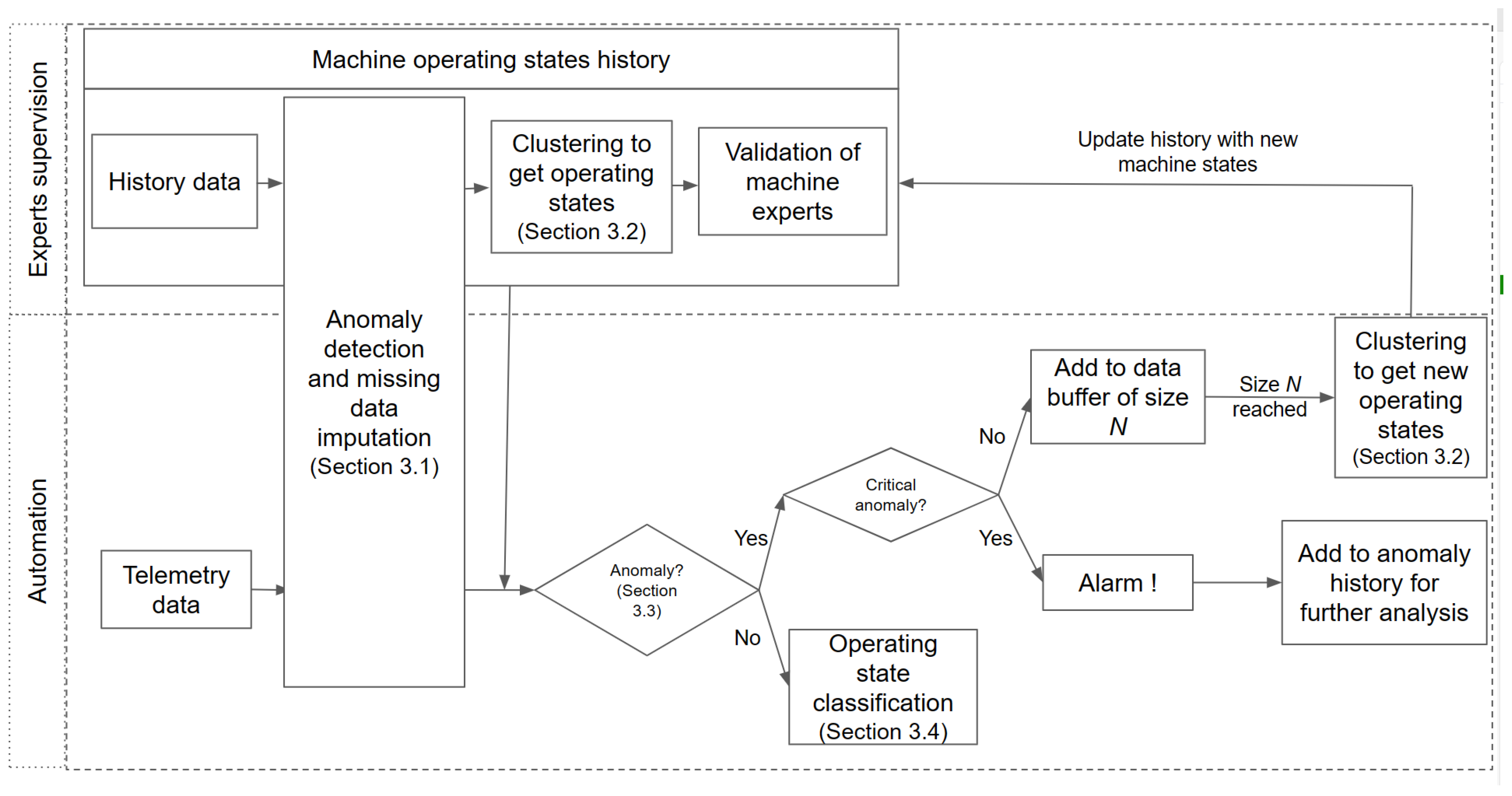
• The learning phase focuses on establishing the first reference machines’ operating states from historical data. This phase is also called “Experts supervision level”, where discussions and validations from the machine experts are needed in some analyses. This part preprocesses and clusters history data to obtain a proposal of machine operating states. The machine experts then review, adjust, and validate the proposal to obtain the machine operating states.

This learning phase starts with a set of historical machine operating data, which typically contains data quality issues including outliers, redundant data, and missing data. The “Anomaly Detection and Missing Data” module (Section 3.1) aims to address these significant data quality issues. Subsequently, the module “Clustering to get Operating States” (Section 3.2) handles the preprocessed dataset to identify the machine’s operational states. These proposed operational states are then subject to review, adjustment, and validation by machine experts to establish the final machine operating states. These labeled operating states serve as the reference points for classifying new observations during the real-time exploitation phase.

• The second part, “real-time exploitation”, or “Automation level”, is almost entirely automated. Telemetry data come from sensors, PLC, etc. The imputation module (“Anomaly Detection and Missing Data”) fills in missing data if necessary. Then, based on historical data, if the telemetry data have abnormal behavior (“Anomaly detection” module, Section 3.3), the procedure classifies it as a candidate for new operating states or triggers an alarm depending on the severity. These anomalies will be added to anomaly history for further analysis. On the other hand, if the telemetry data have normal behavior, the classification module will tag it into one of the historical operating states. Because the real-word dataset has unbalanced class problems, the module “Operating state classification” (Section 3.4) consists of ensemble learning classifiers to enhance the accuracy of the classification.

The upcoming sections will provide a detailed representation of each module within the suggested framework. These modules have been designed to tackle data quality issues such as missing data, the emergence of novel operating states, and unbalanced class problems. The approach aims to comprehensively manage and mitigate these challenges, ensuring the robust and effective functioning of the IIoT technology framework in the detection and monitoring of machine operational states.

3.1. Missing Data Imputation Module

One of the foundational steps in the proposed data monitoring process is data preprocessing, where the data’s quality, consistency, and reliability are established. This step involves various tasks, including outlier detection, handling, and addressing missing data. Detecting and managing outliers is vital for ensuring the integrity of the dataset by identifying and mitigating potentially erroneous or anomalous data points. In addition, missing data imputation techniques are applied to handle gaps in the dataset caused by various factors. Successful data preprocessing sets the stage for subsequent analysis, as it produces a clean and well-structured dataset that can yield meaningful insights into the underlying processes.

Indeed, outlier detection methods are often subjective and context-dependent. Collaborative efforts between data scientists and domain-specific experts are essential in this process. While statistical techniques like Z-scores and the Interquartile Range method lay the foundation for identifying outliers, domain experts contribute their invaluable practical knowledge to define the thresholds, categorize outliers, and provide insights into variable interactions. This synergy between statistical rigor and domain expertise enhances outlier detection accuracy and contextual understanding.

Missing data imputation involves filling in or estimating values for data points absent or incomplete within a dataset. The proposed framework offers a spectrum of imputation techniques, from straightforward median imputation to advanced methods such as K-nearest Neighbors, Density Estimation, Expectation Maximization, Random Forest, and Stochastic Regression imputation. By making a wide range of imputation methods available, users can choose the most appropriate imputation technique to suit the data at hand, leading to more robust and accurate results.

3.2. Identification of the Process Reference States

3.2.1. Dimensionality Reduction

In the context of IIoT, having a substantial volume of available measurements and various monitoring variables for each machine is expected. It often extends to around 20 parameters or more. Analyzing such high-dimensional data is a time-consuming and resource-intensive task. Additionally, the curse of dimensionality is a considerable problem in machine learning. The high number of features increases the complexity of models and hence reduces their performance. As a result, dimensionality reduction techniques are applied to condense the dataset’s feature set while retaining essential information.

Principal Component Analysis is a statistical procedure using an orthogonal transformation to convert a numerical data matrix of potentially correlated variables into a set of uncorrelated linear variables called principal components. To reduce the data dimension, PCA projects each data point onto only the first few principal components (PCs) to obtain lower-dimensional data while preserving as much information as possible. The first principal components are the directions that maximize the projected data variance [75]. In this study, the number of principal components is defined to preserve at least 80% of the total variance of the initial data.

3.2.2. Machine Operational Regimes

The subsequent step is to identify the machine’s operational regimes by analyzing collected data. Machine operating regimes reflect its physical response, diagnostic parameters, and real-time information. Therefore, detecting operating mode will likely improve the performance of several further analyses, such as online fault detection and predictive maintenance. The operational regimes can be obtained by finding the number of clusters in the dataset.

K-means clustering is an unsupervised learning algorithm that proposes a “similarity-based calculation” criterion between the operating unit’s similar operating behaviors and the reference units using Euclidian distance; the algorithm clusters observations with similar operating behaviors into a similar group. Then, the idea is to identify reference units whose behaviors can characterize the machine operating group [76].

Following the identification of operational regimes using clusters, the detection results represent the value range distribution of key machine parameters. Each operating state will be associated with specific parameter value ranges, clearly describing the machine’s behavior under different conditions. These results are then subject to a rigorous examination, adjustment, and verification process led by machine field experts.

3.3. Anomaly Detection and History Updating—Novel Class Detection

With the Industrial Internet of Things (IIoT) implementation, data continuously arrive and need to be processed in the stream. The data stream is preprocessed and classified by classification algorithms to reflect the machine’s instant operating state and health condition. One of the most challenging problems of streaming data classification is “concept drift”, where the data distribution changes in time [4]. That implies the concept that data change over time, and the classification model needs to be updated regularly to reflect the most recent concept. However, another major problem that data stream classification techniques need to handle is “concept-evolution”: the emergence of novel classes.

In real-world data stream classification problems, novel classes may appear at any time in the stream. The classification models cannot detect the novel class (misclassified) until they are trained with labeled instances of the novel class. So, to avoid misclassification of the novel class, the anomaly detection method is applied to data before entering the classification model. It detects outliers that deviate from the “normal class”. Outliers can be distinguished into two types:

• Critical outliers are considered as “danger” or “fault” for the machine operating state. Such outliers are considered as early signs of failure that usually lead to faults or machine breakdown.
• Novel class outliers contain outliers having strong cohesion among themselves. They possess the potential to form a new class regarding “concept-evolution”.

Hence, the contribution of the anomaly detection method is twofold: fault detection and novel class emergence. The most commonly used anomaly detection approaches can be categorized into statistics, clustering, and isolation-based approaches to the best of our knowledge [77].

• Statistics-based approaches construct a model that represents the normal behavior of the dataset. The new incoming data are considered anomalous if they do not match the model or have a very low probability of corresponding to the model [78].
• Clustering and the nearest neighbors approach use the proximity between observations to detect abnormal data. The clustering approach splits the dataset into different clusters as a function of the similarity between the data. Then, it considers the most distant cluster as an anomaly cluster [79]. The nearest neighbors approach calculates the distance between all of the observations in the dataset. It considers new incoming data as an anomaly if it is far from its k nearest neighbors [80] or has the fewest neighbors in a predefined radius r [81].
• The isolation-based approach aims to isolate abnormal observations from the dataset. The anomalous data have two characteristics. First, they have significantly different behavior compared to normal data. Second, they have a very small proportion in the whole dataset. So, the anomalies are likely to be rapidly isolated from the normal dataset [82].

3.4. Operational State Classification Using Ensemble Learning

3.4.1. Unbalanced Classes

In real-world datasets, the issue of imbalanced operating states is a critical concern. It arises when some states occur more frequently than others, potentially leading to biased model predictions. In fields like industrial processes, rare states, such as equipment shutdowns or transitions, can hold crucial information, making it essential to address this imbalance for accurate decision making.

As most of the machine learning algorithms were designed with the assumption of an equal number of examples for each class, unbalanced datasets pose a challenge for the classification models. If the imbalance ratio is extreme, the learning algorithm may sometimes consider the minority class as an outlier or noise and end up dropping them [83]. That leads to poor predictive performance, specifically for the shutdown and transition states.

3.4.2. Mixture Design Weight Ensemble

In Section 2, the study provides an overview of the state of the art in ensemble learning to improve classifier accuracy in unbalanced class distributions. Among the various ensemble techniques, The voting method emerges as a commonly used approach. The voting method aims to efficiently create a weighted scoring system that combines the contributions of individual classifiers. This study introduces a novel approach for optimizing the weights of these participating classifiers. By treating these classifiers as components in a mixture, the study explores the application of a novel simplex–centroid mixture design to obtain experimental weight sets. This approach provides a systematic and data-driven method for enhancing the combination of classifier contributions, strengthening the effectiveness of ensemble learning in class imbalance.

A mixture design is a kind of design of experiments (DOE) which regards each variable as an independent factor. Then, the independent factors are the proportions of different components of a mixture. For example, to optimize the strength of a mixture of concrete, a material engineer searches for an appropriate blend of cement, sand, gravel, and water. Therefore, the strength of the concrete depends on the proportions of the individual material components present in the mix. Applying to this study, the approach aims to maximize the precision, recall, and F1-score by searching for the proportions of the base classifiers’ contributions in ensemble learning. It employs the mixture design to discover the combinations of weights of base classifiers.

The DOE applies a simplex coordinate system, specially simplex–centroid design, to find the optimal weights of participant classifiers. The simplex–centroid mixture designs were first introduced by Scheffe [84] and now are one of the most used standard mixture designs for fitting standard models. The experimental region forms a simplex, a geometric figure with one more vertex than the number of dimensions in these designs. The centroid of the domain corresponds to the mixture with equal proportions for all components. It takes experimental points at the border of the experimental domain. These points are evenly spaced along the coordinates, representing factors. It defines a simplex–centroid design by $(k,m)$, where each of the k components can take on $m+1$ equally spaced levels from 0 to 1, and all possible combinations of the proportions from Equation (1). So, in a $(k,m)$ simplex–centroid design, the total number of points is given in Equation (2).

$$x_i=0,\frac{1}{m},\frac{2}{m},\dots ,\frac{m-1}{m},1;\forall i=1,2,\dots ,k$$

(1)

$$\frac{(k+m-1)!}{m!(q-1)!}$$

(2)

Figure 2 shows illustrations for $(3,2)$ and $(3,3)$ simplex–centroid designs.

To apply a simplex–centroid design in the voting ensemble method, the approach takes the following steps. First, it conducts all the experiments in the mixture design. The method collects and matches as pairs response data with the proportions of base classifiers to build up the dataset. Then, based on the dataset, it can use tools such as regression analysis to build the response prediction models. After making the response prediction models, optimization tools such as mathematical programming techniques [85,86] can be used to maximize some responses (accuracy, recall, or F1-score) by adjusting base classifiers’ weights.

3.4.3. Operating State Classification Module

The operating state classification module implements a plethora of machine learning models for the operating state classification. First of all, it employs the three most widely used classifiers: K-nearest neighbors (KNN), Support Vector Machine (SVM), and Random Forest (RF):

• KNN classifier: It works on the premise that data points having similar attributes will be located closer to each other than data points having dissimilar characteristics. For each query, KNN estimates its relative distances from a specified number of neighboring data points (K) closest to the query. Then, KNN sorts the K-nearest neighboring data points in ascending order of their distances from the query point and classifies the query points according to the mode of the K-nearest data point labels [87].
• SVM classifier: It creates and uses hyperplanes as a decision boundary to be able to classify a query into its correct category class. The hyperplanes are the extreme cases of each data class (known as support vectors), which help define the class boundary. The algorithm attaches a penalty to every point located on the other side of its class across a particular hyperplane. It then explores several hyperplane solutions and selects the best class boundary that maximizes the separation margin between classes [88].
• RF classifier: It consists of multiple decision trees. A decision tree is a set of hierarchical decisions that leads to a classification result. The tree has “root” nodes at the top. Then, it splits into branches based on certain feature-based conditions. Each branch may further split into sub-branches based on more specific sub-feature conditions. The splitting of branches may continue until they reach the leaf node, which is the final classification decision, and no further splitting is needed. For each query, each decision tree in the random forest votes for one of the classes to which the input belongs. Then, the RF will take the vote for the class with the most occurrence as the final prediction [89].

Then, the module employs ensemble learning approaches and cost-sensitive learning methods to handle the problem of imbalance classes and improve the predictive performance:

• It combines the classification output of KNN, SVM, and RF using three voting ensemble approaches—hard voting, soft voting, and mixture design weights—to obtain three classifiers, called “HARD_VOTING”, “SOFT_VOTING”, and “MIXTURE_VOTING”, respectively.
• It uses SMOTE to oversample minority classes, then trains KNN, SVM, and RF on the oversampled complete dataset to obtain three classifiers, “KNN_SMOTE”, “SVM_SMOTE”, and “RF_SMOTE”, respectively.
• It applies cost-sensitive learning methods on SVM and RF to obtain “SVM_COST” and “RF_COST”, respectively. The classifiers put higher costs for misclassifying minority classes than majority classes.

The module evaluates the classification accuracy of eleven classifiers: KNN, SVM, RF, HARD_VOTING, SOFT_VOTING, MIXTURE_VOTING, KNN_SMOTE, SVM_SMOTE, RF_SMOTE, SVM_COST, and RF_COST. It trains and tests the classifiers with the complete train/test datasets and the imputed train/test datasets.

4. Application to Industrial Manufacturing: Glass Wool Production

The research is within the context of an innovative project, Smart InUse, from 2021 to 2023. The project aims to develop advanced predictive and preventive maintenance programs, enhance product quality, and optimize processes. It relies on data from intelligent sensors, dedicated algorithms, and artificial intelligence for analysis to achieve these objectives. This study, in particular, uses Industrial Internet of Things (IIoT) technologies to identify and monitor the operational status of equipment used in the production of glass wool, with a specific focus on a curing oven at the end of the insulation manufacturing chain [90]. The study introduces a comprehensive framework for managing data, covering data acquisition, preprocessing, and machine multi-class classification. This project represents a collaborative effort between the University of Technology of Compiègne and its industrial partners, ALFI Technologies [91] and Cetim [92].

4.1. Data Acquisition

One of the essential steps in data-driven approaches is acquiring, storing, and preprocessing data. It helps to provide reliable data processing for the further analysis. In the context of the project Smart InUse, the data collected every minute from various smart sensors mounted on the curing oven have been stored, building a rich and vast dataset. It contains information of one year of production. The dataset includes different variables representing the processes’ state and other variables reporting the product’s specification.

The curing oven consists of different components such as conveyor belts, curing oven zones, burners, and fans. Generally, the curing oven zone includes five or six discrete horizontal oven zones or stages, each comprising its heat source to form a continuous oven. Each oven zone has its gas burner, serving as a heat source, and a recirculating fan, circulating hot air through the oven. The curing oven also has two exhaust fans to remove the solvent-laden air from the oven and draw fresh air.

The conveyor belts move the fiberglass mat through the curing oven zone to cure the binder. The conveyor belts include a top and a bottom belt. To accommodate products of different thicknesses, operators adjust the distance between these two belts (conveyor height).

To monitor the operating states of different components of ovens, the study collected data on process variables (parameters). These variables consist of conveyor speed, conveyor height, recirculating fan speed, exhaust fan speed, the electricity consumption of conveyors, gas consumption of oven, curing oven zones’ temperature and the number of vibrators, spinners in production. In addition to process variables, the data concerning product variables are also collected. These variables consist of the density, thickness, and net weight of the product. There are relations between the process and product variables, such as the conveyor’s speed condition and the product density. This sums up more than twenty variables describing the curing oven operating states.

4.1.1. Missing Data

In the context of project Smart InUse, the missing data are a typical challenge. It involves sensor failure or disconnection, and some variables have a considerable missing rate of up to 40%. Figure 3 gives an overview of the incompleteness rate of the dataset. In the following paragraphs, the impact of missing data and several statistical approaches are presented to handle incomplete data.

Some researchers prefer the deletion technique, which excludes observations with missing elements from the analysis to clean the dataset. This method is known as list-wise or case-wise deletion [93]. However, although the incomplete observations may contain missing elements, they are not information-free. Deleting inconvenient observations will reduce the information and make the analysis less efficient. In our study, the list-wise deletion reduces 2/3 observations of the dataset. Therefore, the loss of information can be considerable.

4.1.2. Application of the Proposed Framework to the Curing Oven

As described in Section 4.1, the project collected data of the curing oven process variables and the product variables. The process variables consist of conveyor speed, conveyor height, recirculating fan speed, exhaust fan speed, the electricity consumption of conveyors, gas consumption of oven, curing oven zones’ temperature, and the number of vibrators in production. The product variables consist of product density, thickness, and net weight to control the processing product’s quality. This covers a total of more than twenty variables describing the curing oven operating states. To reduce the dimension of data, the project applies PCA to obtain lower-dimensional data while preserving at least 80% of the total variance of the initial data.

In the presented study, the curing oven has five operating states: three production states, one machine shutdown state, and one transition state. Compared to the three production states, the oven shutdown state and its transition are infrequent occurrences of unexpected equipment breakdown and unplanned or planned maintenance. The impact of curing oven shutdown on business can be important. During this study, the collected datasets present most of the three production states and a minority of the shutdown and transition states. Given the extreme class imbalance, there is a risk that the learning algorithm may erroneously classify the minority class as an outlier or noise, potentially leading to their exclusion. This situation results in suboptimal predictive performance, especially concerning the shutdown and transition states. Therefore, the framework requires an ensemble learning approach to enhance the unbalanced class classification.

The study collects data from February 2021 to March 2022. The train dataset was sampled from February 2021 to August 2021. The test dataset was from September 2021 to March 2022 and is divided into 7 datasets. First, the machine field experts examine each dataset to remove outliers, fill in missing data, and label machine operating states. The dataset treated by the machine expert will be considered as the complete dataset in our numerical experiences. Then, the study uses a raw dataset with all missing data to evaluate the impact of missing data on the operating states’ classification.

The study undergoes a two-step process for evaluation. Initially, multiple classifiers are tested on the complete dataset. In the subsequent step, various imputation methods are employed to address missing data within the raw dataset. The classifiers are then re-applied to the imputed dataset. Our primary focus is on assessing the classification accuracy from three perspectives: comparing accuracy between the complete and imputed datasets to gauge the impact of missing data, evaluating the classification accuracy and execution time across different imputation methods, and examining the robustness of classifiers in the presence of missing data. Figure 4 provides an overview of the overall framework for the numerical experiments.

Table 1. The incompleteness rate (%) of each dataset.

Data Set	Gaz Consumpt		Exhaust Fan Speed		Fan Speed Zone 1		T° Zone 1		Electricity Consumpt
	Missing	Longest	Missing	Longest	Missing	Longest	Missing	Longest	Missing	Longest
Train	4.5	0.55	4.5	3.2	12.4	2.3	3	0.5	28.5	2.47
Test 1	5.5	0.6	7.8	3.1	11.1	2.2	5	1.1	12.5	5
Test 2	4.4	0.5	9.7	2.5	14.7	2.9	19.3	1.5	31.5	3.3
Test 3	6.75	0.65	3.29	0.5	7	1.2	11.5	2.5	12.3	3.2
Test 4	15.5	0.59	8.5	3.1	13.9	3.1	6.3	0.4	13.7	4.3
Test 5	5.9	0.7	5.8	1.2	10.1	2.8	2.5	0.4	15.7	2.5
Test 6	3.13	0.41	3.5	0.9	12.3	3.6	17.1	2.1	14.5	2.3
Test 7	2.7	0.64	5.1	2.2	8.2	1.1	1.7	0.1	17.5	3.1

Missing stands for the missing rate (%) of the variable over time horizon. Longest stands for the longest consecutive time interval of the missing data.

gives an overview of the incompleteness rate for all datasets. This study has one train dataset and seven test datasets. The table only illustrates some important variables: gas consumption, exhaust fan speed, fan speed zone 1, temperature zone 1, and electricity consumption. For each variable, it gives the incompleteness rate (Missing) and the longest time interval of missing data (Longest). The incompleteness rate is the ratio (%) of total missing data periods over the time horizon. The “Longest” columns give the longest consecutive time interval of missing data. It represents the duration of the consecutive time interval by its ratio (%) over time horizon duration. For example, a dataset has 1000 data points. A variable whose “Missing”$=10\%$ and “Longest”$=5\%$ has in total 100 missing data points and 50 consecutive missing data points.

4.2. Numerical Results and Discussions

This section presents experimental results, demonstrating the effectiveness and robustness of the proposed framework. The study compares the proposed methodology with two existing ensemble learning methods: the Histogram Gradient Boosting Classifier (HGBC) and the Extreme Gradient Boosting classifier (XGBoost). To assess the classification performances of these methods, the study employs the weighted accuracy metric.

Weighted accuracy is a metric for evaluating classifier performance in imbalanced class classification. It considers class imbalance by assigning weights to classes based on their relative proportions. It calculates accuracy for each class and then computes a weighted average of these class accuracies, with each weight proportional to the class size. This provides a more balanced assessment of classifier performance, giving more weight to smaller classes.

$$\mathrm{Weighted}\mathrm{Accuracy}=\frac{W_1·{\mathrm{Accuracy}}_1+W_2·{\mathrm{Accuracy}}_2+\dots +W_n·{\mathrm{Accuracy}}_n}{W_1+W_2+\dots +W_n}$$

(3)

where:

• Weighted Accuracy is the overall accuracy score that takes into account class weights.
• $W_1$, $W_2$, …, $W_n$ are the weights assigned to each class. These weights are often calculated as the proportion of instances in each class relative to the total number of instances in the dataset.
• Accuracy${}_1$, Accuracy${}_2$, …, Accuracy${}_n$ are the accuracy scores for each class, calculated as the ratio of true positives for that class to the total number of instances in that class.
• n is the total number of classes.

Figure 5 shows the effect of missing data on classification accuracy. It compares the performance between using the complete dataset and the imputed datasets. Figure 6 gives more details on the classification accuracies between imputation methods. Figure 7 presents the overview of classifiers’ performances.

Table 2. Execution time for imputation methods (in seconds) in the “Learning phase”.

Method	KNN	Kernel	EM	RF	S_Regression
Max	5567.00	2800.00	806.00	10,406.00	61.00
Mean	4426.86	2311.86	696.00	8834.43	42.10
$\sigma$	1106.70	478.16	100.53	1319.03	13.59
Min	2973.00	1531.00	535.00	7256.00	21.67

summarizes the execution time for imputation methods (in seconds) in the “Learning phase”. The following sections will discuss the results in detail in the following paragraphs.

4.2.1. The Effect of Missing Data

This section compares the effect of missing data in Figure 5. As the study has up to seven test datasets, it presents the classification accuracy of each classifier in the form of a distribution box plot. There are three columns in the figure: “Complete data”, “Imputed data”, and “Missing data columns”.

The “Complete data” column gives accuracy box plots of classifiers using the “complete” test datasets. As a reminder, the “complete” column includes test datasets whose missing data have been examined and corrected by the machine field experts.

The “Imputed data” column shows the accuracy box plot of classifiers using the imputed datasets, the datasets whose missing data have been filled with different imputation methods. Six imputation methods are applied on seven test datasets. Therefore, each box plot in the “Imputed data” column represents the distribution of classification accuracy of the corresponding classifier on 42 datasets.

The “Missing data” column displays box plots illustrating the classification accuracy of the HGBC and XGBoost classifiers. Notably, these two methods directly classify using incomplete datasets. Each individual box plot within the “Missing data” column represents the distribution of classification accuracy for these two classifiers across the seven incomplete datasets.

Based on Figure 5, the following observations are made:

• All classifiers have high classification accuracy when using the “Complete” test datasets. Their accuracies are at least $82\%$, and in some test datasets, the accuracy is up to $92\%$ for the “HARD_VOTING”. The “RF_SMOTE” and the “RF_COST” box plot show that there is an improvement in the overall classification accuracies of unbalanced classes by using SMOTE and cost-sensitive learning methods in the “Complete” datasets.
• There is a significant performance decrease when using “Imputed” datasets. Most classification accuracies for using “Imputed” datasets are between $80\%$ and $85\%$. For some classifiers, the accuracy decreases to $65\%$, such as for “RF_SMOTE” and “RF_COST”. These two classifiers have high accuracy with the “Complete” dataset. However, their performances fall considerably in cases of imputed data.
  The decrease in performance of RF COST and RF SMOTE can be attributed to multiple factors. RF SMOTE’s synthetic samples can introduce complexity and noise into the dataset, reducing accuracy. RF COST may underperform when the cost matrix is inaccurately defined, failing to reflect true misclassification costs. Both techniques are also prone to overfitting and model complexity issues, especially with high-dimensional or noisy data. These complexities can reduce their accuracy.
• Despite the ability of HGBC and XGBoost to handle incomplete data directly, their performance is significantly inferior to that of other methods. The classification accuracy achieved by these two classifiers varies, frequently falling below $80\%$, and, in the case of XGBoost, declining even to under $60\%$. This observation strongly emphasizes the requirement for employing data imputation methods to address incomplete data before the classification process.

4.2.2. Improvement of Classification Accuracy Using Imputation Methods

This section compares the effect of imputation methods on classification accuracy. The study has seven test datasets and eleven classifiers. Therefore, each box plot in Figure 5 represents the accuracy distribution of 77 experiments. Based on Figure 5, the following observations are made:

• The “Complete” dataset gives the best classification results. On the other hand, the imputed datasets can be divided into three groups according to their performances. The first group comprised methods with the highest accuracy, albeit with a significant computational time requirement. The second group featured methods with slightly lower accuracy but reduced computational demands compared to the first group. The third group encompassed methods that prioritized computational efficiency over accuracy.
• The first group consists of two imputation methods, KNN and RF. They provide accuracy as close as the “Complete” dataset. RF imputation is slightly better than KNN imputation. However, as shown in Table 2, the required execution time of the RF imputation method is nearly twice as long as that required by KNN. Therefore, the KNN imputation method has more performance and time requirement advantages.
• The second group consists of Median imputation, Stochastic regression imputation (S_regression), and EM imputation. Imputation by median value is a straightforward approach. However, in our experiments, its accuracy is as good as with other techniques: S_regression imputation and EM imputation. These three approaches require less execution time and provide over $75\%$ classification accuracy.
• The kernel imputation method provides the worst accuracy among imputation methods. In some datasets, the accuracy may fall to $65\%$. In addition, it is the third most time-consuming approach in our experiments.
• The “Missing data” box plot combines the accuracy results of HGBC and XGBoost when classifying data directly from the incomplete dataset. Despite their computational speed advantages, as demonstrated in the missing data box plot, HGBC and XGBoost often yield accuracy below $70\%$. This observation again emphasizes data imputation methods’ essential role in addressing incomplete data before the classification process.

4.2.3. Ensemble Learning Classifier Performances

This section examines the classifiers’ performances using the “Complete” dataset and imputation approaches. Each column in Figure 7 represents a classifier. Each column has seven box plots corresponding to the “Complete data set” and six “Imputed data sets”. Each box plot shows the distribution of seven experiments corresponding to the seven test datasets. Based on Figure 7, the study carried out can confirm the aforementioned observations:

• The “Complete” dataset gives the best accuracy. “HARD_VOTING”, “RF_SMOTE”, and “RF_SENSITIVE” handle better the unbalanced class classification problem.
• The KNN classifier is more robust to missing data. As can been seen in the KNN columns, there are fewer variations in the box plots than for other classifiers, regardless of imputation methods.
• The KNN and RF imputation approaches give classification accuracies as close as using the “Complete” dataset. These methods ensure the best classification accuracy in the case of missing data. However, their time requirements are significant.
• The Median imputation and Stochastic regression imputation are rapid techniques to handle the missing data in our experiments. They provide over $75\%$ classification accuracies in a short execution time.

5. Conclusions and Perspectives

In the context of the Industrial Internet of Things, the guarantee of the quality of data collected is essential for ensuring reliable and accurate analysis results. The most common problems encountered with real industrial databases are missing data, outliers, anomalies, unbalanced classes, and non-exhaustive historical data. The objective of the paper is to address all these problems at once.

The presented study proposes a general framework for data flow from data acquisition and data preprocessing to machine class classification in two phases: the learning phase and the real-time exploitation phase.

For the learning phase, the missing data problem was handled using several imputation methods. Both outliers and anomalies were detected and eliminated. Two types of outliers were singled out: critical outliers, considered as “danger” or “fault” for the machine, and novel class outliers, which can potentially form a new machine behavior. Dimensionality reduction and clustering methods were applied to detect the operational regimes of the machine. The detected functional states were then discussed, adjusted, and validated with the machine field expert. The final results became the historical databases that characterize the machine states. The entire process was applied in an industrial context.

For the second phase, the problem of unbalanced class classification and the impact of missing data on classification accuracy were addressed. Eleven machine learning models were implemented for operating state classification. The implementation was carried out on the industrial application case of the SMART InUse project. Seven test datasets were collected during the project. Six imputation methods were used to correct the missing data problem. The classification accuracy was compared between the imputed datasets and the complete datasets to obtain the influence of the missing data.

The main finding highlighted by the study is that using “hard voting” ensemble learning methods to combine several classifiers makes the final classifier more robust to missing data. The KNN imputation method is the best-performing and fastest of the six imputation methods tested. Stochastic regression imputation and EM imputation require lower execution times and provide acceptable classification accuracy. The kernel imputation method provides the worst accuracy in some datasets and is the third most time-consuming approach for the considered dataset.

Another point to discuss in this study is the importance of expertise from the field and operational experience in the preprocessing data phase. The benefit from exchanges of practical experience helps to detect outliers and abnormal data efficiently. The feedback from the machine operator provides valuable information to model the oven operating state’s characteristics. Therefore, the collaboration between data scientists and operational experiences from the field is essential.

For perspective, improvements for the key modules within our framework can enhance their efficiency and effectiveness. In the domain of outlier detection, automating the process further to reduce the reliance on human intervention is a significant goal. It can streamline outlier detection without requiring field experts to fine-tune the process. Integrating deep learning techniques, such as coupled deep learning, offers a promising approach for more robust and complete data recovery in the context of missing data imputation. For operating state detection, improving dimensionality reduction is essential. Traditional PCA primarily captures linear correlations, but adopting Kernel Principal Component Analysis (KPCA) [94] can better represent complex nonlinear relationships within the data, leading to more accurate and robust operating state detection.

As seen previously, the considered process has several operational regimes that are all normal operating states and which are very dependent on the type of product manufactured. All those operating states can be seen as a single reference state. Consequently, the reference state has a non-Gaussian distribution. The next step of this study would be to control such a process (detect and identify a potential drift). To this end, the use of a multivariate approach for a non-Gaussian multidimensional distribution considering a clustering algorithm based on Gaussian mixtures and several $T^2$ multivariate control charts could be studied.

References

1. Rüßmann, M.; Lorenz, M.; Gerbert, P.; Waldner, M.; Justus, J.; Engel, P.; Harnisch, M. Industry 4.0: The future of productivity and growth in manufacturing industries. Boston Consult. Group 2015, 9, 54–89. [Google Scholar]
2. Shahin, K.I.; Simon, C.; Weber, P.; Theilliol, D. Input-Output Hidden Markov Model for System Health Diagnosis Under Missing Data. In Proceedings of the 2020 28th Mediterranean Conference on Control and Automation (MED), Saint-Raphaël, France, 15–18 September 2020; pp. 556–561. [Google Scholar]
3. He, H.; Garcia, E.A. Learning from imbalanced data. IEEE Trans. Knowl. Data Eng. 2009, 21, 1263–1284. [Google Scholar]
4. Gama, J.; Žliobaitė, I.; Bifet, A.; Pechenizkiy, M.; Bouchachia, A. A survey on concept drift adaptation. ACM Comput. Surv. (CSUR) 2014, 46, 1–37. [Google Scholar] [CrossRef]
5. Tan, X.; Gao, C.; Zhou, J.; Wen, J. Three-way decision-based co-detection for outliers. Int. J. Approx. Reason. 2023, 160, 108971. [Google Scholar] [CrossRef]
6. Iglewicz, B.; Hoaglin, D.C. Volume 16: How to Detect and Handle Outliers; Quality Press: Milwaukee, WI, USA, 1993. [Google Scholar]
7. Whaley, D.L., III. The Interquartile Range: Theory and Estimation. Electronic Theses and Dissertations, East Tennessee State University, Johnson City, TN, USA, 2005. [Google Scholar]
8. Yang, X.; Latecki, L.J.; Pokrajac, D. Outlier detection with globally optimal exemplar-based GMM. In Proceedings of the 2009 SIAM International Conference on Data Mining, Sparks, NV, USA, 30 April–2 May 2009; pp. 145–154. [Google Scholar]
9. Degirmenci, A.; Karal, O. Efficient density and cluster based incremental outlier detection in data streams. Inf. Sci. 2022, 607, 901–920. [Google Scholar] [CrossRef]
10. He, Z.; Xu, X.; Deng, S. Discovering cluster-based local outliers. Pattern Recognit. Lett. 2003, 24, 1641–1650. [Google Scholar] [CrossRef]
11. Angiulli, F.; Pizzuti, C. Fast outlier detection in high dimensional spaces. In Proceedings of the European Conference on Principles of Data Mining and Knowledge Discovery, Helsinki, Finland, 19–23 August 2002; pp. 15–27. [Google Scholar]
12. Zhang, K.; Hutter, M.; Jin, H. A new local distance-based outlier detection approach for scattered real-world data. In Proceedings of the 13th Pacific-Asia Conference on Knowledge Discovery and Data Mining (PAKDD-09), Bangkok, Thailand, 27–30 April 2009; pp. 813–822. [Google Scholar]
13. Breunig, M.M.; Kriegel, H.P.; Ng, R.T.; Sander, J. LOF: Identifying density-based local outliers. In Proceedings of the 2000 ACM SIGMOD International Conference on Management of Data, Dallas, TX, USA, 16–18 May 2000; pp. 93–104. [Google Scholar]
14. Tang, J.; Chen, Z.; Fu, A.W.C.; Cheung, D.W. Enhancing effectiveness of outlier detections for low density patterns. In Proceedings of the 6th Pacific-Asia Conference on Advances in Knowledge Discovery and Data Mining, Taipei, Taiwan, 6–8 May 2002; pp. 535–548. [Google Scholar]
15. Kriegel, H.P.; Kröger, P.; Schubert, E.; Zimek, A. LoOP: Local outlier probabilities. In Proceedings of the 18th ACM Conference on Information and Knowledge Management, Hong Kong, China, 2–6 November 2009; pp. 1649–1652. [Google Scholar]
16. Tang, B.; He, H. A local density-based approach for outlier detection. Neurocomputing 2017, 241, 171–180. [Google Scholar] [CrossRef]
17. Liu, F.T.; Ting, K.M.; Zhou, Z.H. Isolation forest. In Proceedings of the 2008 Eighth IEEE International Conference on Data Mining, Pisa, Italy, 15–19 December 2008; pp. 413–422. [Google Scholar]
18. Blomberg, L.C.; Ruiz, D.D.A. Evaluating the influence of missing data on classification algorithms in data mining applications. In Proceedings of the Anais do IX Simpósio Brasileiro de Sistemas de Informação (SBC), João Pessoa, Brazil, 22–24 May 2013; pp. 734–743. [Google Scholar]
19. Acuna, E.; Rodriguez, C. The treatment of missing values and its effect on classifier accuracy. In Classification, Clustering, and Data Mining Applications: Proceedings of the Meeting of the International Federation of Classification Societies (IFCS), Illinois Institute of Technology, Chicago, IL, USA, 15–18 July 2004; Springer: Berlin/Heidelberg, Germany, 2004; pp. 639–647. [Google Scholar]
20. Farhangfar, A.; Kurgan, L.; Dy, J. Impact of imputation of missing values on classification error for discrete data. Pattern Recognit. 2008, 41, 3692–3705. [Google Scholar] [CrossRef]
21. Twala, B. An empirical comparison of techniques for handling incomplete data using decision trees. Appl. Artif. Intell. 2009, 23, 373–405. [Google Scholar] [CrossRef]
22. Buczak, P.; Chen, J.J.; Pauly, M. Analyzing the Effect of Imputation on Classification Performance under MCAR and MAR Missing Mechanisms. Entropy 2023, 25, 521. [Google Scholar] [CrossRef]
23. Gabr, M.I.; Helmy, Y.M.; Elzanfaly, D.S. Effect of missing data types and imputation methods on supervised classifiers: An evaluation study. Big Data Cogn. Comput. 2023, 7, 55. [Google Scholar] [CrossRef]
24. Brown, R.L. Efficacy of the indirect approach for estimating structural equation models with missing data: A comparison of five methods. Struct. Equ. Model. Multidiscip. J. 1994, 1, 287–316. [Google Scholar] [CrossRef]
25. Tutz, G.; Ramzan, S. Improved methods for the imputation of missing data by nearest neighbor methods. Comput. Stat. Data Anal. 2015, 90, 84–99. [Google Scholar] [CrossRef]
26. Titterington, D.; Sedransk, J. Imputation of missing values using density estimation. Stat. Probab. Lett. 1989, 8, 411–418. [Google Scholar] [CrossRef]
27. Di Zio, M.; Guarnera, U.; Luzi, O. Imputation through finite Gaussian mixture models. Comput. Stat. Data Anal. 2007, 51, 5305–5316. [Google Scholar] [CrossRef]
28. Stekhoven, D.J.; Bühlmann, P. MissForest—Non-parametric missing value imputation for mixed-type data. Bioinformatics 2012, 28, 112–118. [Google Scholar] [CrossRef]
29. Little, R.J.; Rubin, D.B. Statistical Analysis with Missing Data; John Wiley & Sons: Hoboken, NJ, USA, 2019; Volume 793. [Google Scholar]
30. Lim, H. Low-rank learning for feature selection in multi-label classification. Pattern Recognit. Lett. 2023, 172, 106–112. [Google Scholar] [CrossRef]
31. Priyadharshini, M.; Banu, A.F.; Sharma, B.; Chowdhury, S.; Rabie, K.; Shongwe, T. Hybrid Multi-Label Classification Model for Medical Applications Based on Adaptive Synthetic Data and Ensemble Learning. Sensors 2023, 23, 6836. [Google Scholar] [CrossRef]
32. Teng, Z.; Cao, P.; Huang, M.; Gao, Z.; Wang, X. Multi-label borderline oversampling technique. Pattern Recognit. 2024, 145, 109953. [Google Scholar] [CrossRef]
33. Lin, I.; Loyola-González, O.; Monroy, R.; Medina-Pérez, M.A. A review of fuzzy and pattern-based approaches for class imbalance problems. Appl. Sci. 2021, 11, 6310. [Google Scholar] [CrossRef]
34. Wong, W.Y.; Hasikin, K.; Khairuddin, M.; Salwa, A.; Razak, S.A.; Hizaddin, H.F.; Mokhtar, M.I.; Azizan, M.M. A Stacked Ensemble Deep Learning Approach for Imbalanced Multi-Class Water Quality Index Prediction. Comput. Mater. Contin. 2023, 76, 1361–1384. [Google Scholar]
35. Asselman, A.; Khaldi, M.; Aammou, S. Enhancing the prediction of student performance based on the machine learning XGBoost algorithm. Interact. Learn. Environ. 2023, 31, 3360–3379. [Google Scholar] [CrossRef]
36. Tarekegn, A.N.; Giacobini, M.; Michalak, K. A review of methods for imbalanced multi-label classification. Pattern Recognit. 2021, 118, 107965. [Google Scholar] [CrossRef]
37. Batista, G.E.; Prati, R.C.; Monard, M.C. A study of the behavior of several methods for balancing machine learning training data. ACM SIGKDD Explor. Newsl. 2004, 6, 20–29. [Google Scholar] [CrossRef]
38. Liu, X.Y.; Wu, J.; Zhou, Z.H. Exploratory undersampling for class-imbalance learning. IEEE Trans. Syst. Man Cybern. Part B (Cybern.) 2008, 39, 539–550. [Google Scholar]
39. Castellanos, F.J.; Valero-Mas, J.J.; Calvo-Zaragoza, J.; Rico-Juan, J.R. Oversampling imbalanced data in the string space. Pattern Recognit. Lett. 2018, 103, 32–38. [Google Scholar] [CrossRef]
40. Charte, F.; Rivera, A.J.; Jesus, M.J.d.; Herrera, F. MLeNN: A first approach to heuristic multilabel undersampling. In Proceedings of the International Conference on Intelligent Data Engineering and Automated Learning, Salamanca, Spain, 10–12 September 2014; pp. 1–9. [Google Scholar]
41. Pereira, R.M.; Costa, Y.M.; Silla, C.N., Jr. MLTL: A multi-label approach for the Tomek Link undersampling algorithm. Neurocomputing 2020, 383, 95–105. [Google Scholar] [CrossRef]
42. Santiago, J.; Claeys-Bruno, M.; Sergent, M. Construction of space-filling designs using WSP algorithm for high dimensional spaces. Chemom. Intell. Lab. Syst. 2012, 113, 26–31. [Google Scholar] [CrossRef]
43. Sobol’, I.M. On the distribution of points in a cube and the approximate evaluation of integrals. Zhurnal Vychislitel’Noi Mat. Mat. Fiz. 1967, 7, 784–802. [Google Scholar] [CrossRef]
44. Bakhvalov, N.S. On the approximate calculation of multiple integrals. J. Complex. 2015, 31, 502–516. [Google Scholar] [CrossRef]
45. Butler, N.A. Optimal and orthogonal Latin hypercube designs for computer experiments. Biometrika 2001, 88, 847–857. [Google Scholar] [CrossRef]
46. Raghavarao, D.; Preece, D. Combinatorial analysis and experimental design: A review of “Constructions and Combinatorial Problems in Design of Experiments” by Damaraju Raghavarao. J. R. Stat. Soc. Ser. D (Stat.) 1972, 21, 77–87. [Google Scholar] [CrossRef]
47. Chawla, N.V.; Bowyer, K.W.; Hall, L.O.; Kegelmeyer, W.P. SMOTE: Synthetic minority over-sampling technique. J. Artif. Intell. Res. 2002, 16, 321–357. [Google Scholar] [CrossRef]
48. Wang, B.X.; Japkowicz, N. Imbalanced data set learning with synthetic samples. In Proceedings of the IRIS Machine Learning Workshop, Ottawa, ON, Canada, 9 June 2004; Volume 19, p. 435. [Google Scholar]
49. Han, H.; Wang, W.Y.; Mao, B.H. Borderline-SMOTE: A new over-sampling method in imbalanced data sets learning. In Proceedings of the International Conference on Intelligent Computing, Hefei, China, 23–26 August 2005; pp. 878–887. [Google Scholar]
50. Pradipta, G.A.; Wardoyo, R.; Musdholifah, A.; Sanjaya, I.N.H. Radius-SMOTE: A new oversampling technique of minority samples based on radius distance for learning from imbalanced data. IEEE Access 2021, 9, 74763–74777. [Google Scholar] [CrossRef]
51. He, H.; Bai, Y.; Garcia, E.A.; Li, S. ADASYN: Adaptive synthetic sampling approach for imbalanced learning. In Proceedings of the 2008 IEEE International Joint Conference on Neural Networks (IEEE World Congress on Computational Intelligence), Hong Kong, China, 1–8 June 2008; pp. 1322–1328. [Google Scholar]
52. Tepvorachai, G.; Papachristou, C. Multi-label imbalanced data enrichment process in neural net classifier training. In Proceedings of the 2008 IEEE International Joint Conference on Neural Networks (IEEE World Congress on Computational Intelligence), Hong Kong, China, 1–8 June 2008; pp. 1301–1307. [Google Scholar]
53. Zhang, M.L. ML-RBF: RBF neural networks for multi-label learning. Neural Process. Lett. 2009, 29, 61–74. [Google Scholar] [CrossRef]
54. Sun, K.W.; Lee, C.H. Addressing class-imbalance in multi-label learning via two-stage multi-label hypernetwork. Neurocomputing 2017, 266, 375–389. [Google Scholar] [CrossRef]
55. Pouyanfar, S.; Wang, T.; Chen, S.C. A multi-label multimodal deep learning framework for imbalanced data classification. In Proceedings of the 2019 IEEE Conference on Multimedia Information Processing and Retrieval (MIPR), San Jose, CA, USA, 28–30 March 2019; pp. 199–204. [Google Scholar]
56. Sozykin, K.; Protasov, S.; Khan, A.; Hussain, R.; Lee, J. Multi-label class-imbalanced action recognition in hockey videos via 3D convolutional neural networks. In Proceedings of the 2018 19th IEEE/ACIS International Conference on Software Engineering, Artificial Intelligence, Networking and Parallel/Distributed Computing (SNPD), Busan, Republic of Korea, 27–29 June 2018; pp. 146–151. [Google Scholar]
57. Li, C.; Shi, G. Improvement of Learning Algorithm for the Multi-instance Multi-label RBF Neural Networks Trained with Imbalanced Samples. J. Inf. Sci. Eng. 2013, 29, 765–776. [Google Scholar]
58. Kittler, J.; Hatef, M.; Duin, R.P.; Matas, J. On combining classifiers. IEEE Trans. Pattern Anal. Mach. Intell. 1998, 20, 226–239. [Google Scholar] [CrossRef]
59. Ho, T.K. Random decision forests. In Proceedings of the 3rd International Conference on Document Analysis and Recognition, Montreal, QC, Canada, 14–16 August 1995; Volume 1, pp. 278–282. [Google Scholar]
60. Wolpert, D.H. Stacked generalization. Neural Netw. 1992, 5, 241–259. [Google Scholar] [CrossRef]
61. Ho, T.K.; Hull, J.J.; Srihari, S.N. Decision combination in multiple classifier systems. IEEE Trans. Pattern Anal. Mach. Intell. 1994, 16, 66–75. [Google Scholar]
62. Kuncheva, L.I.; Rodríguez, J.J. A weighted voting framework for classifiers ensembles. Knowl. Inf. Syst. 2014, 38, 259–275. [Google Scholar] [CrossRef]
63. Yin, X.; Liu, Q.; Pan, Y.; Huang, X.; Wu, J.; Wang, X. Strength of stacking technique of ensemble learning in rockburst prediction with imbalanced data: Comparison of eight single and ensemble models. Nat. Resour. Res. 2021, 30, 1795–1815. [Google Scholar] [CrossRef]
64. Winata, G.I.; Khodra, M.L. Handling imbalanced dataset in multi-label text categorization using Bagging and Adaptive Boosting. In Proceedings of the 2015 International Conference on Electrical Engineering and Informatics (ICEEI), Denpasar, Bali, Indonesia, 10–11 August 2015; pp. 500–505. [Google Scholar]
65. Sun, Y.; Kamel, M.S.; Wong, A.K.; Wang, Y. Cost-sensitive boosting for classification of imbalanced data. Pattern Recognit. 2007, 40, 3358–3378. [Google Scholar] [CrossRef]
66. Cao, P.; Liu, X.; Zhao, D.; Zaiane, O. Cost sensitive ranking support vector machine for multi-label data learning. In Proceedings of the International Conference on Hybrid Intelligent Systems, Seville, Spain, 18–20 April 2016; pp. 244–255. [Google Scholar]
67. Wu, G.; Tian, Y.; Liu, D. Cost-sensitive multi-label learning with positive and negative label pairwise correlations. Neural Netw. 2018, 108, 411–423. [Google Scholar] [CrossRef] [PubMed]
68. Witten, I.H.; Frank, E. Data mining: Practical machine learning tools and techniques with Java implementations. Acm Sigmod Rec. 2002, 31, 76–77. [Google Scholar] [CrossRef]
69. Kim, H.; Kim, H.; Moon, H.; Ahn, H. A weight-adjusted voting algorithm for ensembles of classifiers. J. Korean Stat. Soc. 2011, 40, 437–449. [Google Scholar] [CrossRef]
70. Cheon, Y.; Kim, D. Natural facial expression recognition using differential-AAM and manifold learning. Pattern Recognit. 2009, 42, 1340–1350. [Google Scholar] [CrossRef]
71. Sun, B.; Xu, F.; Zhou, G.; He, J.; Ge, F. Weighted joint sparse representation-based classification method for robust alignment-free face recognition. J. Electron. Imaging 2015, 24, 013018. [Google Scholar] [CrossRef]
72. Lu, W.; Wu, H.; Jian, P.; Huang, Y.; Huang, H. An empirical study of classifier combination based word sense disambiguation. IEICE Trans. Inf. Syst. 2018, 101, 225–233. [Google Scholar] [CrossRef]
73. Ren, F.; Li, Y.; Hu, M. Multi-classifier ensemble based on dynamic weights. Multimed. Tools Appl. 2018, 77, 21083–21107. [Google Scholar] [CrossRef]
74. Peng, T.; Ye, C.; Chen, Z. Stacking Model-based Method for Traction Motor Fault Diagnosis. In Proceedings of the 2019 CAA Symposium on Fault Detection, Supervision and Safety for Technical Processes (SAFEPROCESS), Xiamen, China, 5–7 July 2019; pp. 850–855. [Google Scholar]
75. Wold, S.; Esbensen, K.; Geladi, P. Principal component analysis. Chemom. Intell. Lab. Syst. 1987, 2, 37–52. [Google Scholar] [CrossRef]
76. Jain, A.K.; Dubes, R.C. Algorithms for Clustering Data; Prentice-Hall, Inc.: Upper Saddle River, NJ, USA, 1988. [Google Scholar]
77. Togbe, M.U.; Chabchoub, Y.; Boly, A.; Barry, M.; Chiky, R.; Bahri, M. Anomalies detection using isolation in concept-drifting data streams. Computers 2021, 10, 13. [Google Scholar] [CrossRef]
78. Yamanishi, K.; Takeuchi, J.I.; Williams, G.; Milne, P. On-line unsupervised outlier detection using finite mixtures with discounting learning algorithms. Data Min. Knowl. Discov. 2004, 8, 275–300. [Google Scholar] [CrossRef]
79. Masud, M.; Gao, J.; Khan, L.; Han, J.; Thuraisingham, B.M. Classification and novel class detection in concept-drifting data streams under time constraints. IEEE Trans. Knowl. Data Eng. 2010, 23, 859–874. [Google Scholar] [CrossRef]
80. Angiulli, F.; Fassetti, F. Detecting distance-based outliers in streams of data. In Proceedings of the Sixteenth ACM Conference on Conference on Information and Knowledge Management, Lisbon, Portugal, 6–10 November 2007; pp. 811–820. [Google Scholar]
81. Pokrajac, D.; Lazarevic, A.; Latecki, L.J. Incremental local outlier detection for data streams. In Proceedings of the 2007 IEEE Symposium on Computational Intelligence and Data Mining, Honolulu, HI, USA, 1–5 April 2007; pp. 504–515. [Google Scholar]
82. Liu, F.T.; Ting, K.M.; Zhou, Z.H. Isolation-based anomaly detection. ACM Trans. Knowl. Discov. Data (TKDD) 2012, 6, 1–39. [Google Scholar] [CrossRef]
83. Dangut, M.D.; Skaf, Z.; Jennions, I. Rescaled-LSTM for predicting aircraft component replacement under imbalanced dataset constraint. In Proceedings of the 2020 Advances in Science and Engineering Technology International Conferences (ASET), Dubai, United Arab Emirates, 4 February–9 April 2020; pp. 1–9. [Google Scholar]
84. Scheffé, H. Experiments with mixtures. J. R. Stat. Soc. Ser. B (Methodol.) 1958, 20, 344–360. [Google Scholar] [CrossRef]
85. Montgomery, D.C. Design and Analysis of Experiments; John Wiley & Sons: Hoboken, NJ, USA, 2017. [Google Scholar]
86. Khuri, A.I.; Mukhopadhyay, S. Response surface methodology. Wiley Interdiscip. Rev. Comput. Stat. 2010, 2, 128–149. [Google Scholar] [CrossRef]
87. Lopez-Bernal, D.; Balderas, D.; Ponce, P.; Molina, A. Education 4.0: Teaching the basics of KNN, LDA and simple perceptron algorithms for binary classification problems. Future Internet 2021, 13, 193. [Google Scholar] [CrossRef]
88. Chapelle, O.; Haffner, P.; Vapnik, V.N. Support vector machines for histogram-based image classification. IEEE Trans. Neural Netw. 1999, 10, 1055–1064. [Google Scholar] [CrossRef]
89. Pal, M. Random forest classifier for remote sensing classification. Int. J. Remote Sens. 2005, 26, 217–222. [Google Scholar] [CrossRef]
90. Ho, M.H.; Ponchet Durupt, A.; Boudaoud, N.; Vu, H.C.; Caracciolo, A.; Sieg-Zieba, S.; Xu, Y.; Leduc, P. An Overview of Machine Health Management in Industry 4.0. In Proceedings of the 31st European Safety and Reliability Conference, ESREL 2021, Angers, France, 19–23 September 2021; Research Publishing Services: Singapore, 2021; pp. 433–440. [Google Scholar]
91. Alfi. The ALFI Technologies Group: Turnkey Solutions FOR the Intralogistics and the Production of Building Materials. 2021. Available online: http://www.alfi-technologies.com/en/alfi-technologies/le-groupe/ (accessed on 1 June 2021).
92. Cetim. Mission—Cetim—Technical Centre for Mechanical Industry. 2021. Available online: https://www.cetim.fr/en/About-Cetim/Mission (accessed on 1 June 2021).
93. Lin, T.H. A comparison of multiple imputation with EM algorithm and MCMC method for quality of life missing data. Quality Quant. 2010, 44, 277–287. [Google Scholar] [CrossRef]
94. Lee, J.M.; Yoo, C.; Choi, S.W.; Vanrolleghem, P.A.; Lee, I.B. Nonlinear process monitoring using kernel principal component analysis. Chem. Eng. Sci. 2004, 59, 223–234. [Google Scholar] [CrossRef]
Figure 1. The global scheme to exploit the IIotT data in monitoring and detecting machine operational states.
Mathematics 11 04602 g001
Figure 2. Three-component simplex–lattice mixture designs.
Mathematics 11 04602 g002
Figure 3. The overview of the incompleteness rate of dataset.
Mathematics 11 04602 g003
Figure 4. The summary scheme of numerical experiments.
Mathematics 11 04602 g004
Figure 5. Classification performance between classifiers for complete data and imputed data. (The diamond symbol indicates data points outside the majority range of the data).
Mathematics 11 04602 g005
Figure 6. Classification between imputation methods. (The circle symbol indicates data points outside the majority range of the data).
Mathematics 11 04602 g006
Figure 7. Overview of classification performance comparison between classifiers. (The diamond symbol indicates data points outside the majority range of the data.)
Mathematics 11 04602 g007