
A Heavy-Tailed Distribution Based on the Lomax–Rayleigh Distribution with Applications to Medical Data
 , , , and
Abstract
:1. Introduction
2. The Slash Lomax–Rayleigh Model
2.1. Stochastic Representation
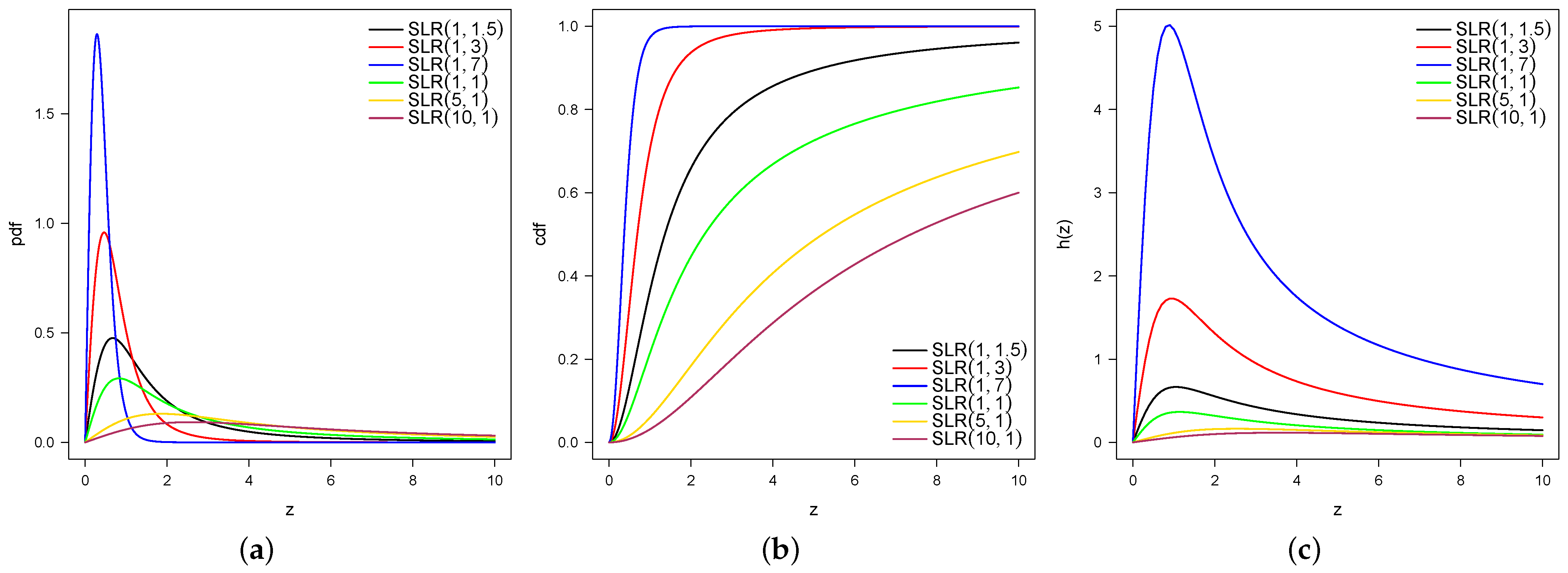
2.2. PDF, CDF, Hazard Function, and Other Properties
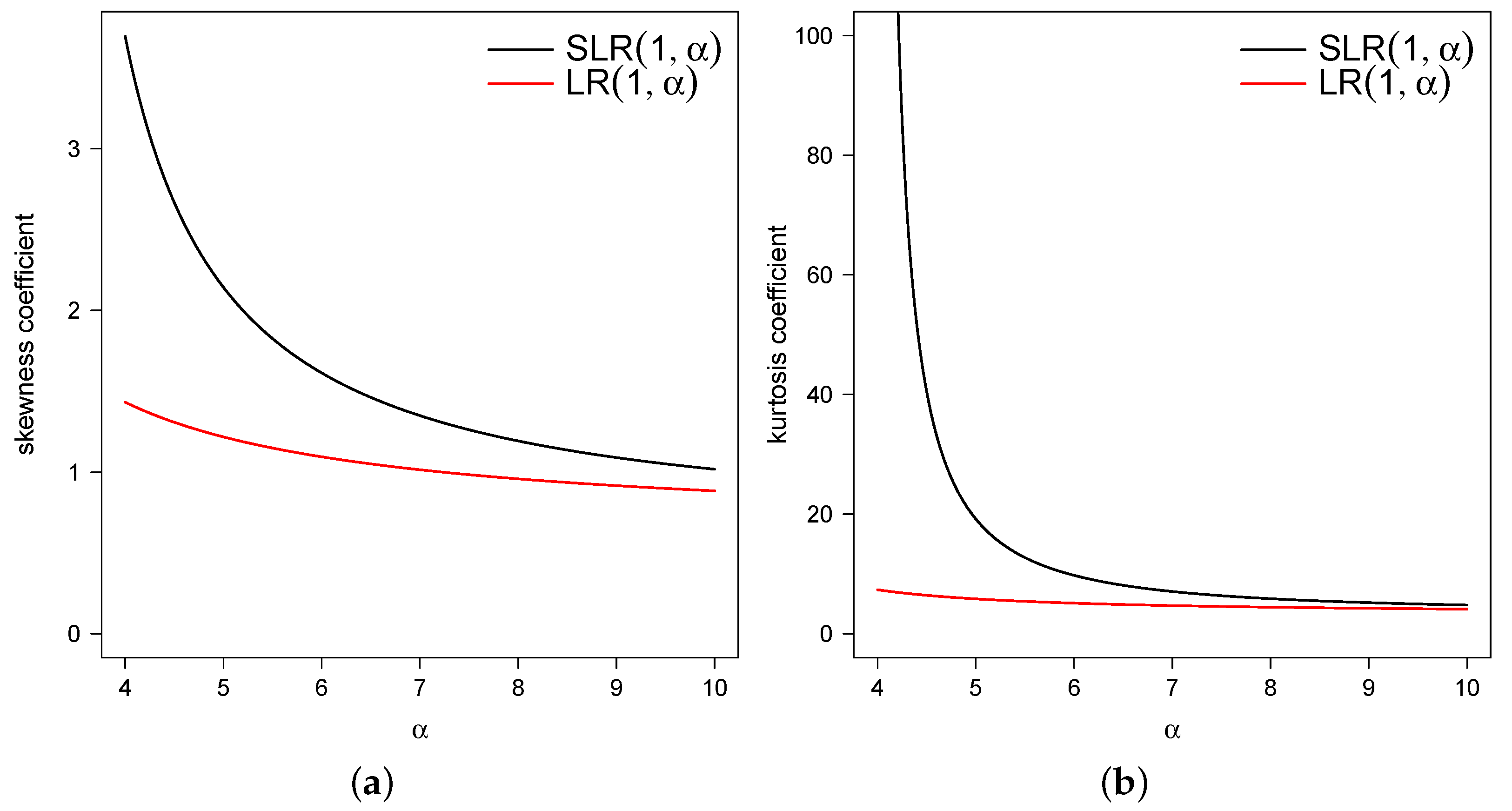
2.3. Moments
- 1.
- 2.
- 3.
- 4.
- 5.
- Var
2.4. Incomplete Moments
2.5. The Lorenz Curve and the Gini Index
2.6. Order Statistics
- 1.
- The PDF of the first-order statistic is given by:
- 2.
- The PDF of the n-th order statistic is given by:
3. Inference
3.1. Moment Estimators
3.2. ML Estimators
3.3. Observed Information Matrix
4. Simulation Study
| Algorithm 1 Simulating values from the distribution |
| 1: Simulate . 2: Calculate . 3: Calculate . 4: Return Z. . |
4.1. Recovery Parameters
4.2. Assessing Model Selection Criteria
5. Applications
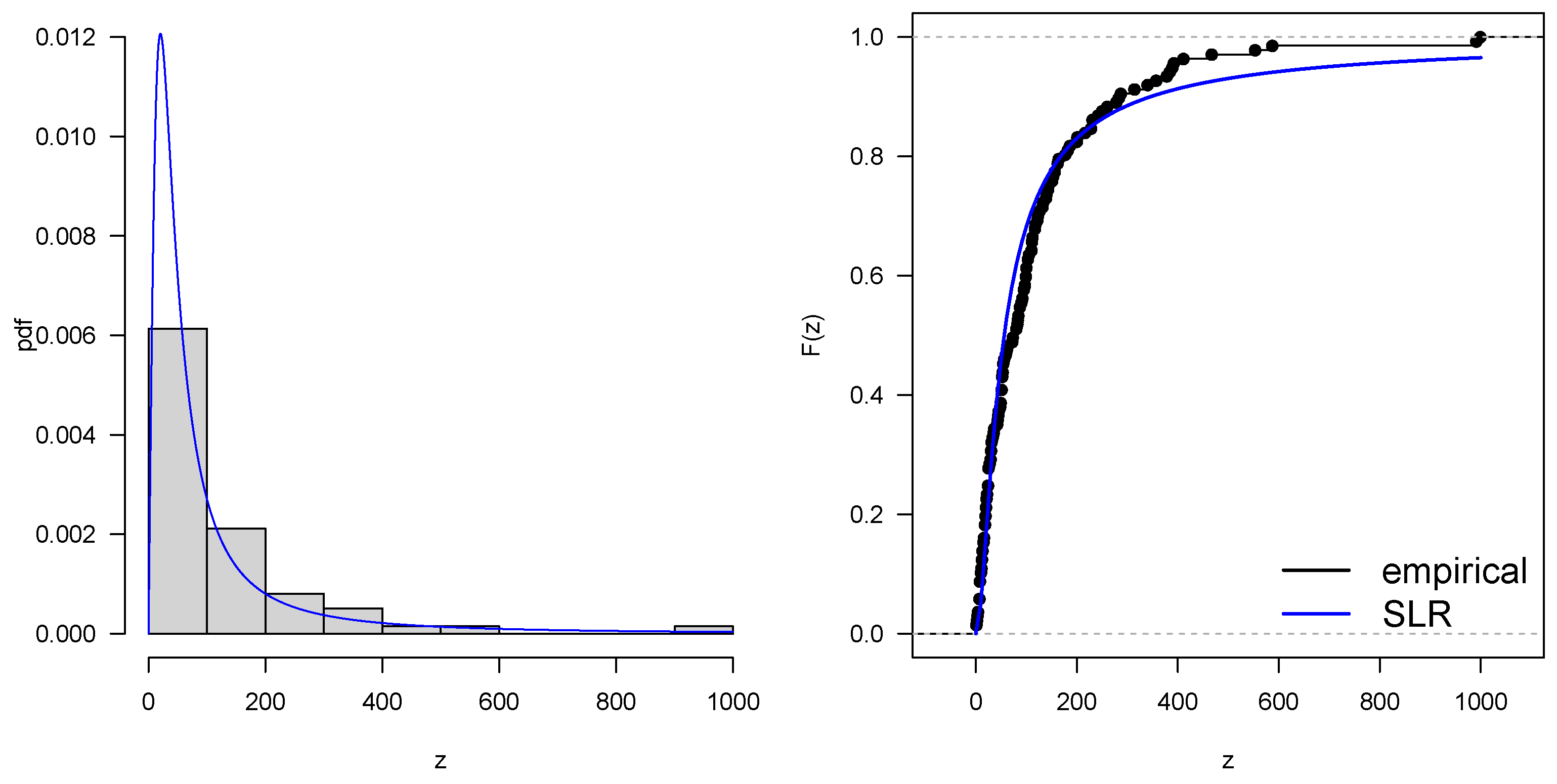
5.1. Application 1
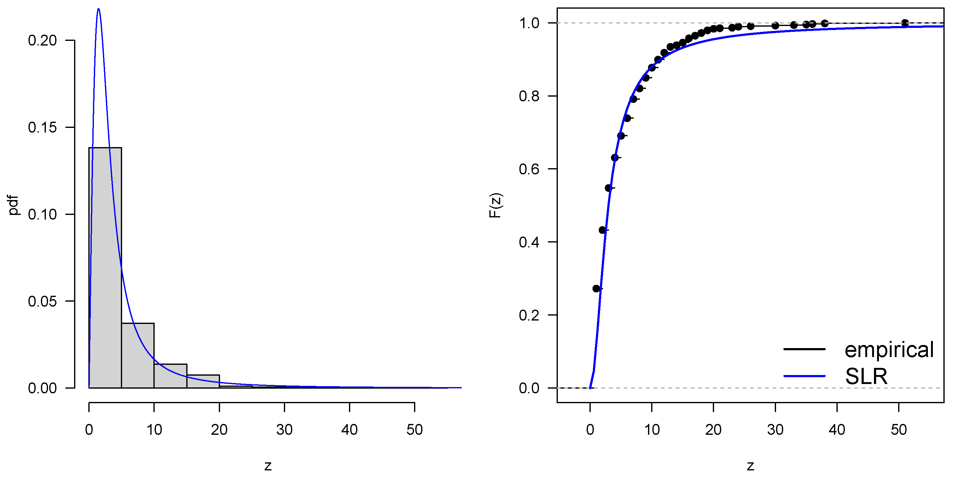
5.2. Application 2
6. Final Discussion
- The SLR distribution has a closed expression and depends on the incomplete beta function.
- The SLR distribution has a heavy right tail.
- The SLR distribution can also be represented as a mixed scale between the LR and beta distributions.
- The CDF, hazard function, moments, and incomplete moments are explicit and are represented by known functions.
- The asymmetry and kurtosis coefficients of the SLR distribution have greater ranges than the coefficients of the LR distribution.
- The applications show that the SLR distribution is a good alternative when the data present positive asymmetry with a heavy right tail; this is confirmed by the AIC and BIC model selection criteria.
Author Contributions
Funding
Institutional Review Board Statement
Informed Consent Statement
Data Availability Statement
Conflicts of Interest
References
- Johnson, N.L.; Kotz, S.; Balakrishnan, N. Continuous Univariate Distributions, 2nd ed.; Wiley: New York, NY, USA, 1995; Volume 1. [Google Scholar]
- Cordeiro, G.M.; Cristino, C.T.; Hashimoto, E.M.; Ortega, E.M. The beta generalized Rayleigh distribution with applications to lifetime data. Stat. Pap. 2013, 54, 133–161. [Google Scholar] [CrossRef]
- Olmos, N.M.; Gómez-Déniz, E.; Venegas, O. The Heavy-Tailed Gleser Model: Properties, Estimation, and Applications. Mathematics 2022, 10, 4577. [Google Scholar] [CrossRef]
- Zhao, J.; Ahmad, Z.; Mahmoudi, E.; Hafez, E.H.; El-Din, M.M.M. A New Class of Heavy-Tailed Distributions: Modeling and Simulating Actuarial Measures. Complexity 2021, 2021, 5580228. [Google Scholar] [CrossRef]
- Riad, F.H.; Radwan, A.; Almetwally, E.M.; Elgarhy, M. A new heavy tailed distribution with actuarial measures. J. Radiat. Res. Appl. Sci. 2023, 16, 100562. [Google Scholar] [CrossRef]
- Afify, A.Z.; Pescim, R.R.; Cordeiro, G.M.; Mahran, H.A. A New Heavy-Tailed Exponential Distribution: Inference, Regression Model and Applications. Pak. J. Stat. Oper. Res. 2023, 19, 395–411. [Google Scholar] [CrossRef]
- Cococcioni, M.; Fiorini, F.; Pagano, M. Modelling Heavy Tailed Phenomena Using a LogNormal Distribution Having a Numerically Verifiable Infinite Variance. Mathematics 2023, 11, 1758. [Google Scholar] [CrossRef]
- Xu, L.; Yao, Q.; Zhang, H. Non-Asymptotic Guarantees for Robust Statistical Learning under Infinite Variance Assumption. J. Mach. Learn. Res. 2023, 24, 1–46. [Google Scholar]
- Venegas, O.; Iriarte, Y.A.; Astorga, J.M.; Gómez, H.W. Lomax-Rayleigh Distribution with an Application. Appl. Math. Inf. Sci. 2019, 13, 741–748. [Google Scholar] [CrossRef]
- Rogers, W.H.; Tukey, J.W. Understanding some long-tailed symmetrical distributions. Stat. Neerl. 2019, 26, 211–226. [Google Scholar] [CrossRef]
- Mosteller, F.; Tukey, J.W. Data Analysis and Regression. A Second Course in Statistics; Addison-Wesley: Reading, MA, USA, 1977. [Google Scholar]
- Kafadar, K. A biweight approach to the one-sample problem. J. Am. Stat. Assoc. 1982, 77, 416–424. [Google Scholar] [CrossRef]
- Wang, J.; Genton, M. The multivariate skew-slash distribution. J. Stat. Plan. Inference 2006, 136, 209–220. [Google Scholar] [CrossRef]
- Gómez, H.W.; Quintana, F.A.; Torres, F.J. A new family of slash-distributions with elliptical contours. Stat. Probab. Lett. 2007, 77, 717–725. [Google Scholar] [CrossRef]
- Olmos, N.M.; Varela, H.; Gómez, H.W.; Bolfarine, H. An extension of the half-normal distribution. Stat. Pap. 2012, 53, 875–886. [Google Scholar] [CrossRef]
- Olmos, N.M.; Varela, H.; Bolfarine, H.; Gómez, H.W. An extension of the generalized half-normal distribution. Stat. Pap. 2014, 55, 967–981. [Google Scholar] [CrossRef]
- Acitas, S.; Arslan, T.; Senoglu, B. Slash Maxwell Distribution: Definition, Modified Maximum Likelihood Estimation and Applications. Gazi Univ. J. Sci. 2020, 33, 249–263. [Google Scholar] [CrossRef]
- Gómez, H.J.; Gallardo, D.I.; Santoro, K.I. Slash Truncation Positive Normal Distribution and its Estimation Based on the EM Algorithm. Symmetry 2021, 13, 2164. [Google Scholar] [CrossRef]
- Barrios, L.; Gómez, Y.M.; Venegas, O.; Barranco-Chamorro, I.; Gómez, H.W. The Slashed Power Half-Normal Distribution with Applications. Mathematics 2022, 10, 1528. [Google Scholar] [CrossRef]
- Arendarczyk, M.; Kozubowski, T.J.; Panorska, A.K. Slash distributions, generalized convolutions, and extremes. Ann. Ins. Stat. Math. 2023, 74, 593–617. [Google Scholar] [CrossRef]
- Rolski, T.; Schmidli, H.; Schmidt, V.; Teugel, J. Stochastic Processes for Insurance and Finance; John Wiley & Sons: Hoboken, NJ, USA, 1999. [Google Scholar]
- Lorenz, M.O. Methods of measuring the concentration of wealth. J. Am. Stat. Assoc. 1905, 9, 209–219. [Google Scholar]
- Gini, C. On the measurement of concentration and variability of characters. Metron 2005, 63, 1–38. [Google Scholar]
- Gini, C. Measurement of inequality of incomes. Econ. J. 1921, 31, 124–126. [Google Scholar] [CrossRef]
- Balakrishnan, N.; Cohen, C.A. Order Statistics and Inference: Estimation Methods; Statistical Modeling and Decision Science; Elsevier Science: Amsterdam, The Netherlands, 1991. [Google Scholar]
- Casella, G.; Berger, R.L. Statistical Inference; Duxbury: Pacific Grove, CA, USA, 2002. [Google Scholar]
- R Core Team. R: A Language and Environment for Statistical Computing; R Foundation for Statistical Computing: Vienna, Austria, 2023; Available online: https://www.R-project.org/ (accessed on 12 October 2023).
- MacDonald, I.L. Does Newton-Raphson really fail? Stat. Methods Med. Res. 2014, 23, 308–311. [Google Scholar] [CrossRef] [PubMed]
- Akaike, H. A new look at the statistical model identification. IEEE Trans. Autom. Control 1974, 19, 716–723. [Google Scholar] [CrossRef]
- Schwarz, G. Estimating the dimension of a model. Ann. Stat. 1978, 6, 461–464. [Google Scholar] [CrossRef]
- Vuong, Q.H. Likelihood Ratio Tests for Model Selection and non-nested Hypotheses. Econometrica 1989, 57, 307–333. [Google Scholar] [CrossRef]
- Kalbfleisch, J.D.; Prentice, R.L. The Statistical Analysis of Failure Time Data; John Wiley and Sons: New York, NY, USA, 1980. [Google Scholar]
- Therneau, T. A Package for Survival Analysis in R; R Package Version 3.5-7; R Foundation for Statistical Computing: Vienna, Austria, 2023; Available online: https://cran.r-project.org/package=survival (accessed on 12 March 2023).
- Castillo, J.S.; Rojas, M.A.; Reyes, J. A More Flexible Extension of the Fréchet Distribution Based on the Incomplete Gamma Function and Applications. Symmetry 2023, 15, 1608. [Google Scholar] [CrossRef]
- Schumacher, M.; Bastert, G.; Bojar, H.; Hübner, K.; Olschewski, M.; Sauerbrei, W.; Schmoor, C.; Beyerle, C.; Neumann, R.L.; Rauschecker, H.F. Randomized 2×2 trial evaluating hormonal treatment and the duration of chemotherapy in node-positive breast cancer patients. German Breast Cancer Study Group. J. Clin. Oncol. 1994, 12, 2086–2093. [Google Scholar] [CrossRef]

| 5 | 6 | 7 | 10 | 20 | ||
|---|---|---|---|---|---|---|
| 2.142 | 1.826 | 1.613 | 1.349 | 1.018 | 0.777 | |
| 19.029 | 12.727 | 9.763 | 7.065 | 4.796 | 3.718 |
| Mode | |
|---|---|
| 1 | 0.824 |
| 3 | 0.462 |
| 5 | 0.348 |
| 7 | 0.288 |
| 9 | 0.251 |
| 12 | 0.215 |
| True Value | ||||||||||||||
|---|---|---|---|---|---|---|---|---|---|---|---|---|---|---|
| Estim. | Bias | SE | RMSE | CP | Bias | SE | RMSE | CP | Bias | SE | RMSE | CP | ||
| 1 | 1 | 0.1437 | 0.4563 | 0.5292 | 0.8970 | 0.0418 | 0.2929 | 0.3174 | 0.9100 | 0.0175 | 0.1730 | 0.1924 | 0.9240 | |
| 0.0270 | 0.1287 | 0.1380 | 0.9210 | 0.0083 | 0.0883 | 0.0902 | 0.9250 | 0.0008 | 0.0534 | 0.0566 | 0.9350 | |||
| 2 | 0.1739 | 0.4910 | 0.6288 | 0.9340 | 0.0793 | 0.3130 | 0.3483 | 0.9450 | 0.0278 | 0.1858 | 0.1968 | 0.9470 | ||
| 0.1136 | 0.3858 | 0.4428 | 0.9500 | 0.0587 | 0.2576 | 0.2832 | 0.9520 | 0.0181 | 0.1561 | 0.1622 | 0.9490 | |||
| 3 | 0.2152 | 0.5945 | 0.7354 | 0.9300 | 0.1068 | 0.3532 | 0.3980 | 0.9480 | 0.0399 | 0.2046 | 0.2087 | 0.9590 | ||
| 0.2703 | 0.8385 | 1.0074 | 0.9620 | 0.1357 | 0.5158 | 0.5614 | 0.9560 | 0.0530 | 0.3061 | 0.3159 | 0.9550 | |||
| 10 | 1 | 1.0928 | 4.6147 | 4.9835 | 0.9200 | 0.6209 | 3.0987 | 3.1515 | 0.9430 | 0.3235 | 1.9047 | 1.9843 | 0.9490 | |
| 0.0215 | 0.1316 | 0.1361 | 0.9560 | 0.0091 | 0.0904 | 0.0908 | 0.9460 | 0.0075 | 0.0569 | 0.0570 | 0.9480 | |||
| 2 | 1.8062 | 4.9530 | 6.2205 | 0.9420 | 0.6775 | 3.0951 | 3.3442 | 0.9550 | 0.3048 | 1.8784 | 1.9640 | 0.9510 | ||
| 0.1246 | 0.3904 | 0.4693 | 0.9610 | 0.0508 | 0.2559 | 0.2748 | 0.9540 | 0.0200 | 0.1571 | 0.1630 | 0.9480 | |||
| 3 | 2.3098 | 6.0022 | 7.1093 | 0.9380 | 1.0098 | 3.5086 | 3.6259 | 0.9560 | 0.3798 | 2.0444 | 2.1095 | 0.9540 | ||
| 0.3110 | 0.8537 | 1.0266 | 0.9570 | 0.1285 | 0.5135 | 0.5295 | 0.9550 | 0.0468 | 0.3054 | 0.3111 | 0.9520 | |||
| LR | W | IG | SHN | LR | W | IG | SHN | LR | W | IG | SHN | |||
|---|---|---|---|---|---|---|---|---|---|---|---|---|---|---|
| 1 | 1 | AIC | 0.64 | 1.00 | 0.84 | 0.92 | 0.64 | 1.00 | 0.95 | 0.97 | 0.65 | 1.00 | 1.00 | 1.00 |
| BIC | 0.64 | 1.00 | 0.84 | 0.92 | 0.64 | 1.00 | 0.95 | 0.97 | 0.65 | 1.00 | 1.00 | 1.00 | ||
| Vuong | 0.33 | 0.89 | 0.20 | 0.45 | 0.35 | 1.00 | 0.43 | 0.59 | 0.39 | 1.00 | 0.83 | 0.86 | ||
| 2 | AIC | 0.47 | 0.98 | 0.84 | 0.97 | 0.48 | 1.00 | 0.94 | 1.00 | 0.50 | 1.00 | 1.00 | 1.00 | |
| BIC | 0.47 | 0.98 | 0.84 | 0.97 | 0.48 | 1.00 | 0.94 | 1.00 | 0.50 | 1.00 | 1.00 | 1.00 | ||
| Vuong | 0.38 | 0.59 | 0.18 | 0.60 | 0.41 | 0.84 | 0.30 | 0.78 | 0.45 | 1.00 | 0.69 | 0.98 | ||
| 3 | AIC | 0.44 | 0.91 | 0.86 | 0.98 | 0.49 | 0.98 | 0.97 | 1.00 | 0.49 | 1.00 | 1.00 | 1.00 | |
| BIC | 0.44 | 0.91 | 0.86 | 0.98 | 0.49 | 0.98 | 0.97 | 1.00 | 0.49 | 1.00 | 1.00 | 1.00 | ||
| Vuong | 0.41 | 0.32 | 0.17 | 0.64 | 0.44 | 0.55 | 0.30 | 0.88 | 0.47 | 0.89 | 0.73 | 0.99 | ||
| 10 | 1 | AIC | 0.62 | 1.00 | 0.83 | 0.94 | 0.61 | 1.00 | 0.96 | 0.97 | 0.64 | 1.00 | 1.00 | 1.00 |
| BIC | 0.62 | 1.00 | 0.83 | 0.94 | 0.61 | 1.00 | 0.96 | 0.97 | 0.64 | 1.00 | 1.00 | 1.00 | ||
| Vuong | 0.31 | 0.91 | 0.21 | 0.48 | 0.32 | 0.99 | 0.47 | 0.60 | 0.37 | 1.00 | 0.84 | 0.89 | ||
| 2 | AIC | 0.48 | 0.97 | 0.83 | 0.97 | 0.52 | 1.00 | 0.94 | 1.00 | 0.51 | 1.00 | 1.00 | 1.00 | |
| BIC | 0.48 | 0.97 | 0.83 | 0.97 | 0.52 | 1.00 | 0.94 | 1.00 | 0.51 | 1.00 | 1.00 | 1.00 | ||
| Vuong | 0.35 | 0.60 | 0.19 | 0.58 | 0.37 | 0.85 | 0.32 | 0.80 | 0.38 | 1.00 | 0.71 | 0.99 | ||
| 3 | AIC | 0.41 | 0.92 | 0.85 | 0.98 | 0.45 | 0.98 | 0.96 | 1.00 | 0.47 | 1.00 | 1.00 | 1.00 | |
| BIC | 0.41 | 0.92 | 0.85 | 0.98 | 0.45 | 0.98 | 0.96 | 1.00 | 0.47 | 1.00 | 1.00 | 1.00 | ||
| Vuong | 0.39 | 0.30 | 0.18 | 0.64 | 0.42 | 0.53 | 0.34 | 0.85 | 0.46 | 0.90 | 0.72 | 1.00 | ||
| n | ||||
|---|---|---|---|---|
| 137 |
| Parameter | SLR | LR | SFr | IG |
|---|---|---|---|---|
| 630.939 (223.857) | 1043.268 (855.508) | 0.772 (0.110) | 24.443 (2.953) | |
| 1.029 (0.112) | 0.497 (0.142) | 0.339 (0.037) | 121.829 (23.277) | |
| Log-likelihood | −802.71 | −804.49 | −872.47 | −816.67 |
| AIC | 1609.43 | 1612.99 | 1748.95 | 1637.35 |
| BIC | 1615.27 | 1618.83 | 1754.79 | 1643.19 |
| Vuong test (p-value) | − | −2.60 (0.009) | −13.81 (<0.001) | −2.05 (0.040) |
| n | ||||
|---|---|---|---|---|
| 686 |
| Parameter | SLR | LR | SHN | W |
|---|---|---|---|---|
| 4.715 (0.777) | 5.584 (0.789) | 3.250 (0.238) | 5.156 (0.196) | |
| 1.493 (0.089) | 0.730 (0.052) | 1.926 (0.203) | 1.067 (0.029) | |
| Log-likelihood | −1748.00 | −1749.81 | −1790.61 | −1788.88 |
| AIC | 3500.00 | 3503.61 | 3585.22 | 3581.76 |
| BIC | 3509.07 | 3512.68 | 3594.28 | 3590.82 |
| Vuong test (p-value) | − | −4.18 (<0.001) | −6.88 (<0.001) | −3.78 (<0.001) |
Disclaimer/Publisher’s Note: The statements, opinions and data contained in all publications are solely those of the individual author(s) and contributor(s) and not of MDPI and/or the editor(s). MDPI and/or the editor(s) disclaim responsibility for any injury to people or property resulting from any ideas, methods, instructions or products referred to in the content. |
© 2023 by the authors. Licensee MDPI, Basel, Switzerland. This article is an open access article distributed under the terms and conditions of the Creative Commons Attribution (CC BY) license (https://creativecommons.org/licenses/by/4.0/).
Share and Cite
Santoro, K.I.; Gallardo, D.I.; Venegas, O.; Cortés, I.E.; Gómez, H.W. A Heavy-Tailed Distribution Based on the Lomax–Rayleigh Distribution with Applications to Medical Data. Mathematics 2023, 11, 4626. https://doi.org/10.3390/math11224626
Santoro KI, Gallardo DI, Venegas O, Cortés IE, Gómez HW. A Heavy-Tailed Distribution Based on the Lomax–Rayleigh Distribution with Applications to Medical Data. Mathematics. 2023; 11(22):4626. https://doi.org/10.3390/math11224626
Chicago/Turabian StyleSantoro, Karol I., Diego I. Gallardo, Osvaldo Venegas, Isaac E. Cortés, and Héctor W. Gómez. 2023. "A Heavy-Tailed Distribution Based on the Lomax–Rayleigh Distribution with Applications to Medical Data" Mathematics 11, no. 22: 4626. https://doi.org/10.3390/math11224626