
Optimal Transport and Seismic Rays

Research School of Earth Sciences, The Australian National University, Canberra, ACT 2601, Australia
*
Author to whom correspondence should be addressed.
Mathematics 2023, 11(22), 4686; https://doi.org/10.3390/math11224686
Submission received: 9 October 2023
/
Revised: 29 October 2023
/
Accepted: 16 November 2023
/
Published: 17 November 2023
(This article belongs to the Special Issue Mathematical Modeling in Geophysics: Concepts and Practices)
Abstract
:We present a theoretical framework that links Fermat’s principle of least time to optimal transport theory via a cost function that enforces local transport. The proposed cost function captures the physical constraints inherent in wave propagation; when paired with specific mass distributions, it yields shortest paths in the considered media through the optimal transport plans. In the discrete setting, our formulation results in physically significant optimal couplings, whose off-diagonal entries identify shortest paths in both directed and undirected graphs. For undirected graphs with positive edge weights, commonly used to parameterize seismic media, our method provides solutions to the Eikonal equation consistent with those from the Dijkstra algorithm. For directed negative-weight graphs, corresponding to transportation cost matrices with negative entries, our approach aligns with the Bellman–Ford algorithm but offers considerable computational advantages. We also highlight potential research directions. These include the use of sparse cost matrices to reduce the number of unknowns and constraints in the considered transportation problem, and solving specific classes of optimal transport problems through the Dijkstra algorithm to enhance computational efficiency.
1. Introduction
The origins of optimal transport theory can be traced back to Gaspard Monge in the 18th century [1]. Monge’s initial problem was rooted in practical concerns, specifically the relocation of soil in the context of construction projects. He aimed to determine the most efficient way to move piles of sand to fill holes, while minimizing worker effort. More generally, optimal transport seeks the cheapest way—in terms of transportation cost—of reshaping a mass distribution into another, or of relocating resources from suppliers to consumers.
Over the years, the theory of optimal transport has transcended its original application and nowadays plays a central role in many areas of applied mathematics, including biology, fluid mechanics, image processing, machine learning, inverse and optimization problems [2,3,4,5]. In the field of geophysics, optimal transport found its first application in exploration seismology less than a decade ago [6], and since then, it has garnered increasing attention [7,8,9].
The renewed interest in this theory, particularly within the seismological community, can be largely attributed to optimal transport inducing a metric; this is known as the Wasserstein or optimal-transport distance, and provides a measure of similarity between density functions. The optimal-transport distance carries interesting properties, which render it amenable to seismic data analysis [10]. For example, when associated with specific (transportation) cost functions and normalizations of seismic waveforms, it exhibits robustness to noise and convexity with respect to data translation and dilation [10]. Furthermore, unlike the Euclidean distance—which measures point-wise similarity between seismograms—the Wasserstein distance offers holistic comparisons, considering simultaneously both their amplitude and phase. Overall, these properties have proven beneficial in mitigating cycle-skipping challenges in waveform-inversion tasks [11,12].
While a significant portion of recent geophysical research has delved into the properties of the Wasserstein distance, the physical interpretability of optimal transport plans remains less explored [13]. This study aims to present an unconventional formulation of the optimal transportation problem, conceived from a simple geometric idea linking Fermat’s principle of least time to the optimal-transport distance. This leads us to devise a cost function that—when used in conjunction with particular mass distributions—reflects wave propagation in heterogeneous media, resulting in transport plans with clear physical significance. The thus identified optimal transport plans allow for tracing rays in the given media, yielding, in the discrete case, approximate solutions to the Eikonal equation.
2. Optimal Transport Theory: A Primer
We briefly introduce in this section the mathematical formalism of optimal transport, from Monge’s initial formulation [1] to its generalization by Kantorovich [14]. As anticipated, optimal transport concerns distributions of “mass” or “density”, which represent the supply and demand of resources. While many studies treat these distributions as probability measures [15], we consider general mass distributions without normalization.
2.1. Monge Formulation
Let and be non-negative measures defined over domains X and Y respectively, representing the supply and demand distributions. These are assumed to have the same mass, i.e.,
Monge’s problem seeks a transport map that transforms into and is bijective, ensuring no mass splitting. Among all feasible (mass-preserving) transport maps , the optimal one minimizes the total transportation cost
where denotes the cost of transporting a unit mass from to . (For clarity, throughout this manuscript, we use to denote the set of non-negative real numbers.)
2.2. Kantorovich Formulation
In 1942, Léon Kantorovich provided a relaxation of Monge’s problem by allowing mass to be split and combined during transport [14]. This leads to the concept of the transport plan, which describes how mass is transported from each point in X to each point in Y. A feasible plan, , must satisfy
The optimal plan is then determined by minimizing the total transportation cost over the set of all feasible plans, i.e.,
Commonly [9,13], the cost function is chosen as , leading to the p-Wasserstein distance .
2.3. Discrete Optimal Transport
The continuous formulation of Kantorovitch can be translated into a discrete form by introducing the concept of coupling, which serves as the discrete counterpart of the transport plan. Given a discretization of the domains X and Y into n and m bins, respectively, let and denote the supply and demand vectors, chosen such that . A feasible coupling, , must satisfy
In other words, each entry represents the amount of mass transported from the ith bin in X to the jth bin in Y [15].
Similar to Equation (4), the optimal coupling minimizes the transportation cost, i.e.,
where is the cost of transporting a unit of mass from the ith to the jth bin, and denotes the set of all feasible couplings. Determining amounts to solving a linear programming problem [16], although the optimal solution is not guaranteed to be unique [15].
3. Linking Optimal Transport to Wave Propagation
Wave propagation in elastic media, such as the Earth’s subsurface, results in a continuous flow of energy or, equivalently, a displacement of mass. At high frequencies, where the wavelength is significantly shorter than the scale of heterogeneities in the medium, the continuous wavefront of a propagating seismic wave can be approximated using ray theory [17,18]. In ray theory, waves are represented by rays that travel along paths determined by the medium’s properties, specifically its velocity structure (or its reciprocal, slowness). The corresponding wave travel times are stationary with respect to perturbations in the ray path, a concept rooted in Fermat’s principle.
The link between optimal transport and ray theory becomes clear when we think of the propagation of a seismic wave as a flow of energy within the medium. In the context of optimal transport, such an energy flow can be analogously viewed as a sequential movement of mass. Starting from a source point (representing the hypocenter), mass is successively transported through its immediate neighborhood, progressing from one neighboring point to another, until it eventually reaches a target point (representing, for example, a receiver). This sequence of infinitesimally small transport steps mirrors the wavefront’s continuous advance through the medium.
3.1. Cost Function and Mass Distributions
To formalize the above idea, we first need to choose appropriate mass distributions, defined over the spatial domain , so as to induce a mass flow (in the optimal-transport sense) from to . Here, X is assumed to be connected in the topological sense, i.e., any two points in X can be joined by a continuous path lying entirely within X. An obvious choice for such distributions is
and
requiring a unit of mass to be relocated from to .
Let , where denotes the Euclidean norm, be the -neighborhood (or ball) of any point , with being a small positive real number. Then, we can define the transportation cost function
where denotes the time required for a wave to travel from x to y. Throughout this manuscript, any transport associated with an infinite cost is treated as unallowed, ensuring that the optimal-transport distance remains finite. Since the cost function (8) assigns infinite cost to the transport of mass between non-neighboring points, it strictly enforces local transport, reflecting the physical constraints of wave propagation. Note how this definition departs from “traditional” optimal transport formulations, where mass can be transported across larger distances without prohibitive costs [6,9].
3.2. Existence of the Transport Plan
Proposition 1.
Given the mass distributions (7), defined over the connected domain X, and the cost function (8), there exists a feasible (mass-preserving) transport plan π. This transport plan must involve a continuous path for mass transport between the source, , and the receiver, , within the domain X.
Proof.
To transform into , a unit of mass must be moved from to . Without loss of generality, assume that and are not immediate neighbors, i.e., . By definition, the cost function (8) assigns infinite cost to transport mass between any two non-neighboring points. Since the mass cannot be transported from to directly, it must come from a neighboring point of , say . Transporting mass to from induces a mass deficit at ; in turn, this must be rectified by transporting a unit of mass to from another neighboring point, say .
The described sequence of mass-transport steps, compensating for the mass deficit at successive neighbors, must eventually be traced back to , the original location with a surplus of mass. It follows that a feasible transport plan must involve a sequence of neighboring points that identify a continuous path for mass transport from to within X. The existence of such a continuous path is guaranteed by the connectedness of X, thus concluding the proof. □
3.3. Optimal Transport Plan
It is important to recognize that, while a continuous path for mass transport from to is ensured by Proposition 1, a feasible transport plan is not required to move mass along this path exclusively. In fact, mass transport between neighboring points that do not lie directly on the path from to may still satisfy mass balance; however, since by definition if , such mass movements will necessarily incur higher transportation costs.
Corollary 1.
From the above discussion, we deduce that an optimal transport plan, as defined by Equation (4), must involve mass transport exclusively along a continuous path (as described in Proposition 1) connecting to .
We emphasize that the optimal transport plan is not guaranteed to be unique, i.e., multiple plans associated with the same transportation cost may exist. For instance, consider a medium with uniform slowness everywhere except for a high-slowness region situated along the most direct route from to . This configuration leads to multiple optimal paths for wave propagation that circumvent the high-slowness region. Specifically, due to the symmetry of the problem, two equivalent optimal paths can be identified in the 2-D setting (Figure 1) and infinitely many in 3-D.
3.4. Optimal-Transport Distance as Least Arrival Time
We established that an optimal transport plan always exists, and this involves a continuous path for mass transport connecting and . Building on this foundation, we now aim to demonstrate the following theorem.
Theorem 1.
Proof.
Consider a continuous path P from to within the domain X. We can decompose this path into a sequence of infinitesimally small segments , each lying entirely within an -neighborhood of some point in X. From (8), the transportation cost between neighboring points x and is , where denotes the time required by a wave to travel between the two points. According to Corollary 1, the optimal transport plan must direct mass exclusively along a continuous path that connects and . This is because any deviations or additional mass exchanges across the domain X would increase the total transportation cost.
It follows that the optimal transport plan is the one minimizing , where is the average slowness of the infinitesimal segment . The optimal-transport distance therefore reads
where denotes the set of all continuous paths connecting and . In the context of our formulation, represents a time duration, specifically the cumulative time taken to traverse the path P given the slowness structure. This minimal time, in accordance with Fermat’s principle of least time, represents the propagation time of a wave from to [17]. □
3.5. Tracing Multiple Rays
The mass distributions defined in Equation (7), which we used earlier to trace a wave generated at and recorded at , can be generalized to accommodate N receivers located at . To this end, we introduce the mass distributions
and
where denotes the set of receivers.
Proposition 2.
Under the conditions of Theorem 1, given the mass distributions and from Equation (10), there exists an optimal transport plan. This plan transports mass along continuous paths from to each receiver, with each path being the shortest in terms of wave travel time.
Proof.
To transform into , N units of mass must be redistributed from the source to the receivers , with each receiver receiving one unit. The structure of the cost function (8) requires that each such mass transportation take place along a continuous path, , spanning a sequence of neighborhoods from to . Building on the proof of Proposition 1, the existence of a feasible transport plan is guaranteed by the connectedness of X and the mass excess at the source in . Furthermore, as established in Corollary 1, any mass exchanges in the domain X outside the paths must result in higher transportation costs. It follows that an optimal transport plan will involve transportation of mass exclusively along such continuous paths.
As deduced in Theorem 1, an optimal transport of mass to each receiver minimizes , where denotes an infinitesimal segment of and its slowness. Since the total transportation cost equals the cumulative cost of transporting mass along , an optimal transport plan minimizes . Minimizing h is equivalent to minimizing the individual transportation costs to each receiver, i.e.,
where denotes the set of all continuous paths connecting and . By Theorem 1, the minimal cost (11) is achieved when each corresponds to a path of least propagation time, thus completing the proof. □
Corollary 2.
A direct implication of Proposition 2 is that the optimal-transport distance, , associated with the optimal transport plan (4), equals the cumulative arrival times of the wave at each receiver. Specifically,
where and are the mass distributions from Equations (7a) and (7b), respectively, and the superscript denotes the receiver.
4. Numerical Validation
In this section, we aim to demonstrate that the derived theory can be implemented in computer code using the discrete optimal transport formulation (Section 2.3). While our study focuses on 2-D media discretized through regular grids for simplicity, the foundational principles of our approach—optimal transport and wave propagation—are inherently geometric. As such, they are not limited by dimensionality, allowing our methodology to be applicable in 2-D, 3-D, as well as higher-dimensional spaces.
4.1. Cost Matrix
Consider a 2-D medium discretized through a Cartesian grid with uniform spacing along both dimensions. Let be the medium’s slowness in each of the n pixels identified by the grid (Figure 2a). To implement the theoretical framework from Section 3, a cost matrix is required that restricts mass transport to neighboring nodes and has entries with time as their physical unit.
To construct such a matrix, we define a connected undirected graph, , where the vertex set consists of nodes placed at the center of each pixel, and the edge set connects only neighboring nodes. Here, we consider two nodes to be neighbors if they reside within adjacent pixels (Figure 2a). For instance, with a unitary grid spacing along both dimensions, neighboring nodes would be those within a distance of either 1 (for horizontally or vertically adjacent pixels) or (for diagonally adjacent pixels). Nodes not directly connected by an edge are considered infinitely distant from each other.
Accordingly, let be the distance matrix where each entry is the Euclidean distance between nodes i and j, with () denoting the coordinates of i. Entries corresponding to non-neighboring nodes are set to infinity. Likewise, we introduce a slowness matrix , chosen such that
The slowness and distance matrices allow us to define the cost matrix , with entries
which serves as the discrete counterpart of the cost function (8). In fact, the above definition results in if , if i and j are neighbors (similar to Section 3, denotes the time required by a wave to travel from node i to node j), and otherwise. An example of the structure of is illustrated in Figure 2b.
4.2. Mass Vectors
We emphasize that the cost matrix (14) is determined solely by the medium’s parameterization, via , and its slowness. Conversely, the mass vectors and , which act as the discrete analogs of the supply and demand distributions from Section 3, depend on the locations of the source and receivers. Similar to Equation (10), these are computed by assigning an appropriate amount of mass to each node in the vertex set . In the case of N receivers belonging to the set ,
and
where denotes the coordinates of the source.
4.3. Optimal Coupling and Its Physical Significance
Given the cost matrix (14) and the mass vectors (15), we can compute an optimal coupling , representing the discrete counterpart of the optimal transport plan. This is achieved by solving the linear program (6), subject to the constraints (5).
Recall from Section 3 that, for a connected domain, an optimal transport plan inherently directs mass along paths from the source to the receivers. As established by Theorem 1 and Proposition 2, these paths are the shortest in terms of wave arrival time. This principle is visually reinforced by Figure 3, which presents two examples of optimal couplings associated with the cost matrix shown in Figure 2b and different source–receiver configurations. A characteristic of these couplings is that only a limited number of off-diagonal entries are non-zero. Each such entry represents the amount of mass transported from the ith to the jth position within the discretized domain. When visualized as arrows connecting nodes i and j in the graph (Figure 3b,d), these mass transports delineate “continuous” paths that connect the source to the receivers. Notably, the identified paths often deviate from the most direct routes, bending towards low-slowness regions of the medium to ensure minimal arrival times [19]. This aspect highlights the physical meaning of , making it a tool for ray tracing in heterogeneous media.
4.4. Optimal Coupling as an Eikonal Solver
As established earlier, off-diagonal entries of an optimal coupling relate to wave propagation between adjacent nodes. This intrinsic property can be exploited to obtain approximate solutions to the Eikonal equation
where s denotes the medium’s slowness, and it is emphasized that the wave travel time t to a point x is dependent on the source location .
In our context, solving Equation (16) involves determining the travel time across n discrete locations that define the medium’s parameterization. Based on Proposition 2, this is achieved by positioning a “receiver” at the center of each pixel that discretizes the medium; with , the mass vectors (15) are computed accordingly. The resulting optimal coupling enables the calculation of the wave’s travel time throughout the medium to each node. In fact, its off-diagonal entries, , correspond to fractional paths taken by the wave to propagate from the ith to the jth node. Starting from a given node, this information can be used to trace the ray’s trajectory back to its source, concurrently computing the arrival time as detailed in Algorithm 1.
| Algorithm 1 Retrieve arrival time at a node. |
|
4.5. Accuracy of the Eikonal Solution
To validate our approach, we employ the P-wave component of the Marmousi model [20], a 2-D slowness model known for its complex subsurface structure (Figure 4a). We first select an arbitrary wave-source position (Figure 4b) and define the mass vectors (15) using 432,776 receivers, each corresponding to a pixel in Figure 4a. We then compute the cost matrix (14), based on the known distances between adjacent nodes and the slowness structure as described in Section 4.1. Finally, we retrieve the optimal coupling by solving the linear program (6), subject to the constraints (5).
Figure 4b shows the resulting travel times. Notably, our results are equivalent to those derived from the Dijkstra algorithm [21], given the same parameterization or undirected graph. (We omitted the image from Dijkstra’s algorithm as it is identical to ours within floating-point precision, making its inclusion redundant.) This congruence is a logical outcome of the foundational principles of both methodologies. In fact, our method identifies the most efficient paths for wave propagation through a heterogeneous medium (Theorem 1 and Proposition 2). Likewise, the Dijkstra algorithm inherently determines the shortest paths between nodes in a weighted graph, where the weights represent the traversal cost or time. Consequently, given identical node distributions and travel costs, our approach is to be considered as accurate as the Dijkstra algorithm and, by extension, the shortest-path networks frequently used in the literature for seismic ray tracing [19,22].
5. Beyond Seismic Media
Building on the theoretical framework presented in Section 3, we have thus far focused on media with strictly positive slowness, discretized through undirected graphs. Drawing a parallel between optimal transport and wavefront propagation, we showed that our approach allows for determining shortest paths in the considered graph, yielding the same results as the Dijkstra algorithm. In this section, we shall consider more general cost functions, admitting negative transportation costs. In particular, we aim to show that our method retrieves the shortest paths within directed graphs characterized by the presence of negative edge weights, consistent with the Bellman–Ford algorithm [23].
5.1. Directed Graphs with Negative Edge Weights
Directed graphs with negative edge weights, while not common in seismology, are of significant interest in other disciplines. In seismology, negative weights would imply the existence of media with negative slowness, a non-physical scenario. However, in computer networking, such graphs are able to represent certain paths or connections that offer rewards or credits [24,25]. For instance, in some network protocols, a node might “credit” data packets sent along a particular route, assigning a negative cost to incentivize its use.
Another intriguing application of negative edge weights lies in the route planning for electric vehicles [26,27]. Unlike fossil-fueled ones, electric vehicles can recover energy under certain conditions, such as while decelerating. This capability, known as regenerative braking, allows them to recharge their battery while in motion, resulting in negative costs in terms of energy consumption. In terrains with varied topography, efficient route planning is therefore crucial, as downhill segments offer opportunities for energy recovery through deceleration [28].
In directed graphs with negative weights, the Bellman–Ford algorithm can reliably find the optimal solution to the above shortest-path problems, given two conditions: (i) a viable route between the path’s endpoints exists, and (ii) no negative cycle is present along the route. Here, by “negative cycle”, we refer to the circumstance where traveling in a loop from a node in the graph to the same node results in a net negative or zero cost. (For clarity, such a cycle would be akin to an electric car that, perpetually traveling within a closed trajectory or loop, produces as much or more energy than it consumes, thereby defying the fundamental laws of energy conservation.)
5.2. Negative Transportation Costs
In the continuous setting, let us reconsider the cost function (8), this time allowing for negative transportation costs. Namely,
where is a real-valued function.
Proposition 3.
Consider the cost function (17) and the mass distributions (7), defined over the connected domain X. Under the assumption that no closed trajectory with net negative transportation cost exists in X, the optimal transport plan, as defined by (4), must involve mass transport exclusively along the shortest path between the considered origin, , and destination, .
Proof.
Building upon Proposition 1, any feasible transport plan must involve transportation of mass along a continuous path connecting and , the existence of which is ensured by the connectedness of X and the mass excess at . In the absence of closed paths with net negative cost in X, any transport plan that involves mass exchanges between pairs of neighboring points, or sequences of neighbors throughout closed trajectories, will have a net positive cost. It follows that an optimal transport plan will not involve any mass exchanges across the domain except for those happening along the continuous path connecting origin and destination; in fact, any deviations from this path must necessarily result in higher transportation costs.
Analogous to the reasoning in Theorem 1, the optimal transport plan will favor the least costly route among all continuous connections between the two considered endpoints in X. This route is also known as the shortest path. □
Corollary 3.
Under the conditions of Proposition 3 and considering the mass distributions (10) for multiple destinations, the optimal transport plan corresponds to mass transports along the shortest paths from the origin to each destination. This follows directly from the arguments presented in the proofs of Propositions 2 and 3.
Remark 1.
Throughout our discussion, we considered X as a connected domain, a natural assumption given the inherent physical continuity of seismic media. However, Proposition 3 and Corollary 3 remain valid even for non-connected domains, provided a continuous path exists between the origin and each destination. This observation is relevant in contexts such as electric vehicles traveling across topographic terrains, where domain connectivity may not be guaranteed.
5.3. Energy-Efficient Routes in Topographic Terrains
To validate the proposed framework, we conduct synthetic numerical tests, simulating the navigation of a topographic terrain with an electric vehicle equipped with regenerative braking capabilities. We consider a discretized topographic surface comprising n pixels, with the elevation of the ith pixel corresponding to the ith entry of (Figure 5a).
Drawing from Section 4.1, we define the directed graph , with nodes at each pixel center and edges connecting only neighboring nodes. Based on , we introduce the cost matrix , where each entry is set to zero if and to if i and j are non-neighboring nodes. We choose the remaining entries such that
where denotes the Euclidean distance between nodes i and j, the signed topographic gradient, and the base energy required to travel a unit of distance. The factors and account for the variations in energy requirement during uphill and downhill traversals, respectively.
It is important to note that, although the cost matrix (18) captures the asymmetry in energy consumption due to topographic gradients (Figure 5b), it offers a simplified representation of an electric car’s energy requirement. Here, we employ Equation (18) for illustrative purposes, and arbitrarily set , and .
Analogous to Section 4, we use Equation (15) to define the mass vectors for specific configurations of origin and destinations. In conjunction with the cost matrix (18), we use the mass vectors to compute an optimal coupling , by solving the linear program (6). Figure 5c shows an example of such a coupling; note how the off-diagonal entries of , corresponding to mass transports between nearby nodes, identify a “continuous” path that connects the origin and destination (Figure 5a). Once again, this path deviates from the most direct route to minimize the total transportation or travel cost.
In a second test, we consider a topographic surface finely discretized into n = 62,001 pixels (Figure 6a) and determine the travel cost from a specific origin point (Figure 6b). This is achieved by defining the mass vectors (15) through 62,001 “receivers” (i.e., destinations, each located at a pixel center), which are used to retrieve an optimal coupling. The energy required to reach each destination is then computed via the off-diagonal entries of the optimal coupling as per Algorithm 1. In fact, while Algorithm 1 was introduced in the context of wave propagation to calculate arrival times, here it retrieves an energy cost due to the definition of the cost matrix (18).
Similar to our earlier comparison with the Dijkstra algorithm in Section 4.5, the results presented in Figure 6b closely match (within floating-point precision) those derived from the Bellman–Ford algorithm, given an analogous directed-graph parameterization. This consistency highlights the robustness of our approach, suggesting its reliability in calculating shortest paths in graphs with negative edge weights.
6. Technical and Computational Remarks
A key observation in the transportation problems solved across this manuscript is the “sparsity” of the cost matrices (14) and (18). In fact, most of their entries, and , are infinite (Figure 2b and Figure 5b); these infinite values inherently indicate prohibited mass transports between nodes i and j, ensuring that the corresponding entries in the resulting optimal coupling are zero (Figure 3a,c and Figure 5c). Since such entries in the optimal coupling are known, the sparsity of and significantly reduces the number of decision variables and constraints in the linear-programming problem (6), making it more tractable.
Leveraging the mentioned sparsity, we evaluate the computational efficiency of our approach by computing approximate solutions to the Eikonal Equation (16) based on increasingly larger undirected graphs . In this experiment, each such graph corresponds to a 2-D seismic medium defined by random slowness (0.2–2 s/m) and discretized via a regular grid as described in Section 4.1. For each parameterization, we randomly select a source position and compute the wave arrival times throughout the medium, based on our approach, and the Dijkstra and Bellman–Ford algorithms. We repeat this calculation fifty times to estimate the average running time and standard deviation for each method. Here and throughout the manuscript, we employ the Dijkstra and Bellman–Ford algorithm implementations from the SciPy Python library [29]; for solving the linear program (6), we use the network simplex algorithm [15] provided by the DOcplex Python API [30].
The outcome of this experiment is illustrated in Table 1. Although the Dijkstra algorithm consistently demonstrates superior computational efficiency, our optimal-transport approach exhibits a significant advantage over the Bellman–Ford algorithm. In fact, based on the collected running times, we estimate computational complexities of for the Bellman–Ford algorithm and for solving our transportation problem; this implies that the relative efficiency of our method, compared with the Bellman–Ford algorithm, becomes increasingly evident as the associated graph grows in size.
7. Future Directions and Conclusions
We showed that optimal transport theory can be used to compute shortest paths in heterogeneous media through ad hoc transportation cost functions and mass distributions. In the discrete setting, the derived theoretical framework can be readily translated into computer code and applied to connected graphs with either positive or negative edge weights. For graphs with positive weights, optimal transport provides shortest-path solutions analogous to those obtained from the Dijkstra algorithm. For graphs with negative weights—assuming the absence of negative cycles—our method aligns with the Bellman–Ford algorithm.
The computational tests presented in this study highlight the advantages of our approach over the Bellman–Ford algorithm when dealing with negative-weight graphs, even though these are infrequently encountered in geophysical parameterizations. Consequently, the immediate applicability of our method to seismic ray-tracing problems might be limited, especially given the Dijkstra algorithm’s superior computational efficiency.
Nevertheless, the novel approach introduced here opens potential avenues for future research. One promising direction involves the use of sparse transportation cost matrices, characterized by infinite entries associated with distant node pairs. These matrices inherently produce optimal couplings that emphasize local transport. Furthermore, their sparsity reduces the number of unknowns and constraints in the associated transportation problems, offering computational benefits. This principle might find utility in scenarios where local mass transport is advantageous, or where this constraint provides valid approximations. For instance, sparse cost matrices could facilitate the transformation of regular grids into curvilinear ones through optimal transport, with each grid point’s distortion representing local mass transport.
Another intriguing research direction arises from the established relationship between optimal transport theory and wave propagation. The Dijkstra algorithm, by design, retrieves shortest paths on undirected graphs, with each path consisting of a node sequence originating from the source. In our optimal transport framework, such node sequences are identified by the off-diagonal entries of the optimal couplings. It follows that the Dijkstra algorithm can be employed to derive optimal couplings when the transportation problem is framed as a shortest-path or wave-propagation problem. Given the Dijkstra algorithm’s computational advantage over the network simplex algorithm, this idea can potentially lead to significant speed-ups in the solution of specific classes of transportation problems.
Author Contributions
Conceptualization, F.M.; Methodology, F.M.; Software, F.M.; Formal analysis, F.M.; Writing—original draft, F.M.; Writing—review & editing, F.M. and M.S.; Visualization, F.M.; Supervision, M.S. All authors have read and agreed to the published version of the manuscript.
Funding
We acknowledge support from the Australian Research Council through a Discovery Project (grant number DP200100053).
Data Availability Statement
The Python codes to reproduce the figures in this manuscript are available at https://github.com/fmagrini/ot-rays (accessed on 7 October 2023).
Acknowledgments
We thank the Commonwealth Scientific Industrial Research Organization Future Science Platform for Deep Earth Imaging for support. The authors are also grateful to three anonymous reviewers.
Conflicts of Interest
The authors declare no conflict of interest.
References
- Monge, G. Mémoire sur la Théorie des Déblais et des Remblais. Mem. Math. Phys. Acad. R. Sci. 1781, 666–704. [Google Scholar]
- Santambrogio, F. Optimal Transport for Applied Mathematicians; Birkäuser: Cham, Switzerland, 2015; Volume 55, p. 94. [Google Scholar]
- Kolouri, S.; Park, S.R.; Thorpe, M.; Slepcev, D.; Rohde, G.K. Optimal mass transport: Signal processing and machine-learning applications. IEEE Signal Process. Mag. 2017, 34, 43–59. [Google Scholar] [PubMed]
- Facca, E.; Benzi, M. Fast iterative solution of the optimal transport problem on graphs. SIAM J. Sci. Comput. 2021, 43, A2295–A2319. [Google Scholar]
- Villani, C. Topics in Optimal Transportation; American Mathematical Society: Providence, RI, USA, 2021; Volume 58. [Google Scholar]
- Engquist, B.; Froese, B.D. Application of the Wasserstein metric to seismic signals. Commun. Math. Sci. 2014, 12, 979–988. [Google Scholar] [CrossRef]
- Métivier, L.; Brossier, R.; Merigot, Q.; Oudet, E.; Virieux, J. An optimal transport approach for seismic tomography: Application to 3D full waveform inversion. Inverse Probl. 2016, 32, 115008. [Google Scholar]
- Yang, Y.; Engquist, B. Analysis of optimal transport and related misfit functions in full-waveform inversion. Geophysics 2018, 83, A7–A12. [Google Scholar] [CrossRef]
- Sambridge, M.; Jackson, A.; Valentine, A.P. Geophysical inversion and optimal transport. Geophys. J. Int. 2022, 231, 172–198. [Google Scholar]
- Engquist, B.; Yang, Y. Optimal transport based seismic inversion: Beyond cycle skipping. Commun. Pure Appl. Math. 2022, 75, 2201–2244. [Google Scholar]
- Métivier, L.; Allain, A.; Brossier, R.; Mérigot, Q.; Oudet, E.; Virieux, J. Optimal transport for mitigating cycle skipping in full-waveform inversion: A graph-space transform approach. Geophysics 2018, 83, R515–R540. [Google Scholar]
- Yang, Y.; Engquist, B.; Sun, J.; Hamfeldt, B.F. Application of optimal transport and the quadratic Wasserstein metric to full-waveform inversion. Geophysics 2018, 83, R43–R62. [Google Scholar] [CrossRef]
- Bryan, J.; Frank, W.B.; Audet, P. Capturing seismic velocity changes in receiver functions with optimal transport. Geophys. J. Int. 2023, 234, 1282–1306. [Google Scholar] [CrossRef]
- Kantorovich, L.V. On the translocation of masses. Dokl. Akad. Nauk. USSR 1942, 37, 199–201. [Google Scholar] [CrossRef]
- Peyré, G.; Cuturi, M. Computational optimal transport: With applications to data science. Found. Trends Mach. Learn. 2019, 11, 355–607. [Google Scholar]
- Vanderbei, R.J. Linear Programming; Springer: Berlin/Heidelberg, Germany, 2020. [Google Scholar]
- Cervenỳ, V. Seismic Ray Theory; Cambridge University Press: Cambridge, UK, 2001; Volume 110. [Google Scholar]
- Aki, K.; Richards, P.G. Quantitative Seismology; University Science Books: Sausalito, CA, USA, 2002. [Google Scholar]
- Rawlinson, N.; Sambridge, M. Seismic traveltime tomography of the crust and lithosphere. Adv. Geophys. 2003, 46, 81–199. [Google Scholar]
- Versteeg, R. The Marmousi experience: Velocity model determination on a synthetic complex data set. Lead. Edge 1994, 13, 927–936. [Google Scholar] [CrossRef]
- Dijkstra, E. A note on two problems in connexion with graphs. Numer. Math. 1959, 1, 269–271. [Google Scholar] [CrossRef]
- Moser, T. Shortest path calculation of seismic rays. Geophysics 1991, 56, 59–67. [Google Scholar] [CrossRef]
- Bellman, R. On a routing problem. Q. Appl. Math. 1958, 16, 87–90. [Google Scholar] [CrossRef]
- Mounika, K.; Jyothirmai, N.; Krishna, A.R. Dynamic Routing with Security Considerations. Int. J. Innov. Technol. Explor. Eng. 2012, 1, 2278–3075. [Google Scholar]
- Sulaiman, O.K.; Siregar, A.M.; Nasution, K.; Haramaini, T. Bellman Ford algorithm—In Routing Information Protocol (RIP). J. Phys. Conf. Ser. 2018, 1007, 012009. [Google Scholar] [CrossRef]
- Abousleiman, R.; Rawashdeh, O. A Bellman-Ford approach to energy efficient routing of electric vehicles. In Proceedings of the 2015 IEEE Transportation Electrification Conference and Expo (ITEC), Dearborn, MI, USA, 14–17 June 2015; pp. 1–4. [Google Scholar]
- Garcia, A.G.; Tria, L.A.R.; Talampas, M.C.R. Development of an energy-efficient routing algorithm for electric vehicles. In Proceedings of the 2019 IEEE Transportation Electrification Conference and Expo (ITEC), Detroit, MI, USA, 19–21 June 2019; pp. 1–5. [Google Scholar]
- Perger, T.; Auer, H. Energy efficient route planning for electric vehicles with special consideration of the topography and battery lifetime. Energy Effic. 2020, 13, 1705–1726. [Google Scholar]
- Virtanen, P.; Gommers, R.; Oliphant, T.E.; Haberland, M.; Reddy, T.; Cournapeau, D.; Burovski, E.; Peterson, P.; Weckesser, W.; Bright, J.; et al. SciPy 1.0: Fundamental algorithms for scientific computing in Python. Nat. Methods 2020, 17, 261–272. [Google Scholar] [PubMed]
- IBM. DOcplex Python Modeling API. 2021. Available online: https://www.ibm.com/docs/en/icos/12.9.0?topic=docplex-python-modeling-api (accessed on 1 September 2023).
Figure 1.
Schematic illustration of a 2-D seismic medium characterized by uniform slowness except for a high-slowness region (dark grey) along the most direct route between a seismic source (star) and a receiver (triangle). In this configuration, two stationary ray paths exist (red lines), both corresponding to the least arrival time of the wave at the receiver.
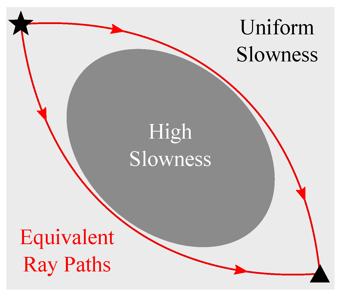
Figure 2.
(a) Discretization of a 2-D medium into a grid with uniform (unitary) spacing along both dimensions, resulting in pixels. Each pixel has a value of slowness and a central node. The red lines highlight the neighbors of the node at (), located in horizontally, vertically, and diagonally adjacent pixels. (b) Cost matrix (14), derived from the discretization in (a). In this case, is a matrix where only a limited number of entries are finite, as indicated by the background color (gray corresponds to non-finite entries). Row and column indexes in (b) correspond to the numbers reported in the lower right of each pixel in (a).

Figure 3.
Optimal couplings, (a,c), associated with the source (star) receivers (triangles) configuration shown in (b,d). The two couplings were computed using the cost matrix in Figure 2b and the mass vectors in Equation (15). Note how each off-diagonal entry corresponds to a mass transport from the ith to the jth node; this is visualized through arrows in (b,d), with colors representing the amount of transported mass.

Figure 4.
(a) P-wave component of the Marmousi model. (b) Wave travel time across the medium, with the red star denoting the source position.
Figure 4.
(a) P-wave component of the Marmousi model. (b) Wave travel time across the medium, with the red star denoting the source position.

Figure 5.
(a) Topographic surface discretized into pixels through a grid with unitary spacing along both dimensions. The yellow star and triangle denote the origin and destination , which are used to calculate the mass vectors (15). (b) Cost matrix (18), derived from the topography in (a). Note the matrix’s asymmetry compared to Figure 2b, which reflects the asymmetric nature of the directed graph introduced in Section 5.3. (c) Optimal coupling , derived from the cost matrix (18) and the mass vectors (15). The shortest path connecting and , as identified by the off-diagonal entries of , is shown in the form of red arrows in panel (a).

Figure 6.
(a) Topographic surface discretized into 62,001 pixels. (b) Energy required to travel from the origin (red star) throughout the terrain, obtained from the optimal coupling as explained in Section 5.3.
Figure 6.
(a) Topographic surface discretized into 62,001 pixels. (b) Energy required to travel from the origin (red star) throughout the terrain, obtained from the optimal coupling as explained in Section 5.3.


Table 1.
Average running time (in ms) and standard deviation for the Dijkstra, Bellman–Ford and optimal-transport (OT) algorithms on undirected graphs with random edge weights, with and denoting the number of graph nodes and edges. The reported times, obtained using a 6-core (AMD Ryzen 5 5600H) laptop with 16 GB of RAM, omit the computations needed to determine the graph weights.
| Dijkstra | Bellman–Ford | OT | ||
|---|---|---|---|---|
| 400 | 2964 | 0.21 ± 0.06 | 1.92 ± 0.42 | 15.58 ± 0.97 |
| 1600 | 12,324 | 0.42 ± 0.01 | 29.60 ± 0.47 | 96.05 ± 2.08 |
| 3600 | 28,084 | 0.87 ± 0.22 | 150.91 ± 2.57 | 195.31 ± 5.22 |
| 6400 | 50,244 | 1.46 ± 0.08 | 480.75 ± 8.84 | 358.32 ± 8.99 |
| 10,000 | 78,804 | 2.36 ± 0.16 | 1184.05 ± 20.83 | 653.19 ± 29.23 |
| 16,900 | 133,644 | 4.27 ± 0.92 | 3383.53 ± 59.46 | 1450.47 ± 33.10 |
| 25,600 | 202,884 | 6.36 ± 0.47 | 7750.18 ± 110.86 | 2715.73 ± 73.76 |
| 40,000 | 317,604 | 10.93 ± 2.65 | 18,968.36 ± 265.16 | 5440.09 ± 147.60 |
| 62,500 | 497,004 | 16.19 ± 0.46 | 46,406.79 ± 755.12 | 11,245.12 ± 799.94 |
Disclaimer/Publisher’s Note: The statements, opinions and data contained in all publications are solely those of the individual author(s) and contributor(s) and not of MDPI and/or the editor(s). MDPI and/or the editor(s) disclaim responsibility for any injury to people or property resulting from any ideas, methods, instructions or products referred to in the content. |
© 2023 by the authors. Licensee MDPI, Basel, Switzerland. This article is an open access article distributed under the terms and conditions of the Creative Commons Attribution (CC BY) license (https://creativecommons.org/licenses/by/4.0/).
Share and Cite
MDPI and ACS Style
Magrini, F.; Sambridge, M. Optimal Transport and Seismic Rays. Mathematics 2023, 11, 4686. https://doi.org/10.3390/math11224686
AMA Style
Magrini F, Sambridge M. Optimal Transport and Seismic Rays. Mathematics. 2023; 11(22):4686. https://doi.org/10.3390/math11224686
Chicago/Turabian StyleMagrini, Fabrizio, and Malcolm Sambridge. 2023. "Optimal Transport and Seismic Rays" Mathematics 11, no. 22: 4686. https://doi.org/10.3390/math11224686
Note that from the first issue of 2016, this journal uses article numbers instead of page numbers. See further details here.