On the State-Feedback Controller Design for Polynomial Linear Parameter-Varying Systems with Pole Placement within Linear Matrix Inequality Regions

Abstract

The present paper addresses linear parameter-varying systems with high-order time-varying parameter dependency known as polynomial LPV systems and their controller design. Throughout this work, a procedure ensuring a state-feedback controller from a parameterized linear matrix inequality (PLMI) solution is presented. As the main contribution of this paper, the controller is designed by considering the time-varying parameter rate as a tuning parameter with a continuous control gain in such a way that the closed-loop eigenvalues lie in a complex plane subset, with high-order time-varying parameters defining the system dynamics. Simulation results are presented, aiming to show the effectiveness of the proposed controller design.

1. Introduction

Nowadays, control systems have been increasing their application in many real problems, rendering an important and vital subsystem within the technology used in our daily life. As a result, this application increment involves an evident control design systems evolution, aiming to face increasingly complex technology challenges. With this, the research community works in different and, in some cases, easier procedures to solve specific control problems, giving rise to new control methodologies. Consequently, and aiming at improving the control systems results, several methods are frequently reported, including those dealing with mathematical approximations for dynamical systems from nonlinear representations. This is the case of linear parameter-varying (LPV) systems [1,2,3,4,5,6], from which nonlinear behaviors can be achieved in such a way that they can be addressed while considering extensions of existing theories for LTI systems with certain restrictions. The previous can be viewed as the main contribution of LPV systems to control systems theory. There exist several representations with different characteristics in the context of LPV systems: descriptor LPV systems [7,8,9], a polytopic LPV representation which interpolates solutions for linear subsystems with their summation viewed as the LPV system’s dynamical behavior [10,11,12,13,14], a quasi-LPV representation from which one can perceive the time-varying dependency as a part of the system state [15,16], and affine LPV systems [17,18]. Within the affine representation, in turn, if the time-varying parameter is defined in polynomial functions of two or greater degrees, a polynomial LPV (PLPV) system should be addressed [19,20,21,22]. As an insight into polynomial LPV systems, let us point out that this particular representation for dynamical systems has been considered, over the years, to approximate real systems such as turbofan engines [23], electrostatically actuated microgrippers [24], 3DOF gyroscopes [25], jet engine compressors [26], flexible robot end-effectors [27], and riderless bicycles [22], among others. Additional important aspects on LPV methodology, in general, can be found in [28,29], presenting data-driven modeling and $H_{\infty }$ control, respectively. Following polynomial LPV systems, the structure for LPV systems from which the present paper’s results are defined becomes important for stating a few concepts involved within their analysis. In addressing PLPV systems stabilization, Lyapunov stability theory is applied to achieve closed-loop stability with a specific controller including decision variables depending on the time-varying parameters, giving rise to a parameterized linear matrix inequality (PLMI) [30,31]. In matrix inequalities theory, in turn, a PLMI is viewed as an infinite-dimension problem because it is time-varying-dependent from a time-varying parameters vector, in the LPV framework. This can be solved using the sum of squares method [32], the discretization method, and a fixed structure search [33]. Within these methods, the fixed structure search allows for the computing of a continuous solution for the PLMI derived from Lyapunov stability theory’s application to polynomial LPV systems. This paper’s results apply this method to compute a continuous control gain by considering a fixed structure for the controller, aiming at placing the closed-loop eigenvalues within a specific subset of the complex plane. Directly related to Lyapunov stability theory, in turn, the so-called LMI regions are usually considered to place eigenvalues within a desired subset of the complex plane. The LMI region is a subset of the complex plane represented by an LMI, allowing for the definition of closed-loop transient criteria, in the case of control design, from a linear matrix inequality. As a result, the problem definition of this paper is related to controller design for PLPV systems with continuous gain, ensuring the closed-loop eigenvalues lie within an LMI region, giving rise to a procedure viewed as an extension of the LMI region methodology towards polynomial LPV systems. Let us point out that although the closed-loop eigenvalues criterion for LPV systems is associated with a slow time-varying parameter variation, the procedure addressed throughout this paper considers the maximum time-varying parameter rate as a tuning parameter for the controller, from the application of Lyapunov stability theory to LPV systems. Including such considerations within the controller design allows us to define a maximum value for the time-varying parameter rate, resulting in an additional degree of freedom involved in the design. As a result, the above provides a maximum time-varying parameter rate that the controller will be able to deal with while controlling the PLPV system, associating it with closed-loop transient responses in terms of eigenvalues located within a specific region of the complex plane. It is important to mention that although there are computer tools for the analysis and computation of PLMIs [34], the proposed methodology considers the matrix relaxation procedure as an analytical design tool, whose development is presented so that the maximum time-varying parameter rate is included within the control design to compute state-feedback control for PLPV systems. With this, consequently, the main contribution of this article refers to a procedure that allows for the placing of closed-loop eigenvalues from what is defined for LTI systems as LMI regions to PLPV systems, considering the time-varying parameter rate as a tuning parameter within the controller design. The result, finally, corresponds to a state-feedback controller whose gains are presented as a polynomial function of the time-varying parameter allocating the closed-loop eigenvalues within an LMI region. Let us point out this contribution concerning [12], research close to that presented within this paper. The proposed method rendering the results shown throughout the present paper is related to polynomial LPV systems, while that contained in [12] is applied to affine LPV systems without considering time-varying parameters with high-order polynomial dependency. In other words, the proposal in [12] considers LPV systems with time-varying dependence in an affine form, computing results by solving its proposal at subsystems formed by the combination of the time-varying parameters’ maximum and minimum values. In general, in the case of two time-varying parameters, a set of four subsystems is that from which the referred results are presented, with its solution associated with the overall LPV system. As for the difference between this particularity and polynomial LPV systems, the results presented throughout this paper do not consider independent subsystems, with handling the PLPV system aiming at computing a continuous time-varying control gain from a system with high time-varying parameter dependency. This is, in turn, enhanced with the LMI regions methodology by taking into account the time-varying parameter rate as a tuning parameter, from which the main contribution of the present paper is defined. With this, finally, the significance of the present results is revealed. The paper structure is as follows: Section 2 contains preliminaries in polynomial LPV systems definition, parameterized LMI, and LMI regions. Section 3 addresses the problem definition to be solved via the controller design and PLMI setup, with issues presented in Section 4. Section 5, in turn, shows the effectiveness of the proposed method by considering a set of LMI regions characterized by different complex plane functions. It presents, additionally, intersections between them or, in other words, the LMI regions’ combination solved simultaneously. Finally, Section 6 provides relevant remarks associated with the proposed method before presenting the conclusion of this paper in Section 7.

2. Notation

Aiming at providing the reader with the variables defining analytical developments within this paper, the

Table 1. Notation.

t	Generalized variable for time.
$\zeta , \beta$	Time-varying parameters.
$x, u, y$	System state and input and output system vectors, respectively.
$A\left(\zeta \right)$, $B\left(\zeta \right)$, $C\left(\zeta \right)$	Time-varying-dependent system matrices.
$i, l, j$	Indexing variables.
${\sum }_{i=1}^k{\sum }_{l=1}^m{\chi }_{\left\{\right[(i-1)m]+l\}}\zeta {\left(t\right)}_l^i$	Generalization for time-varying parameter-dependent matrix.
$K\left(\zeta \right), \overline{K}\left(\zeta \right)$	Control gain.
$V(x,\zeta )$	Time-varying parameter-dependent Lyapunov function.
$Q\left(\zeta \right), \overline{Q}\left(\zeta \right), X\left(\zeta \right)$	Time-varying parameter-dependent matrices for stability purposes.
$M_0, {\gamma }_o, {\gamma }_s$	Parameterized linear matrix inequalities (PLMIs) coefficients.
w	Decision variable in PLMIs.
$\mathbb{C}$	Complex number generalized set.
D	Complex plane subset.
z	Complex number.
$f_D\left(z\right)$	Characteristic function of D.
$M_D(A,X)$	D-stable matrix.
${\chi }_0, L, M, X, A_1, A_2, A_3, B$	Compatible-dimensions constant matrices.
$N_j, Q_1, Q_2, Q_3, {\overline{K}}_0, {\overline{K}}_1, {\overline{K}}_2$	Compatible-dimensions constant matrices.
${\alpha }_0, {\alpha }_1, {\alpha }_2, {\alpha }_3, {\alpha }_4$	Matrix factoring closed-loop coefficients.
$r_j, s$	Relaxed PLMI decision variables.
$J, \nabla$	Jacobian and Hessian matrices, respectively.
$\alpha , r, q, a_1, a_2, \sigma$	LMI regions-defining parameters.
${\Omega }_{1,1}, {\Omega }_{1,2}, {\Omega }_{2,1}, {\Omega }_{2,2}$	Matrix coefficients of factoring disk LMI region.
$N_0, N_{01}, N_{04}, N_{11}, N_{14}$	Matrix coefficients involved in vertical bands LMI region.
${\Gamma }_1, {\Gamma }_2$	Matrix coefficients of factoring horizontal half-strip LMI region.

includes the notation considered in following sections.

3. Preliminaries

3.1. Polynomial Linear Parameter-Varying Systems

Consider the following dynamical system:

$$\begin{array}{c}\dot{x}\left(t\right)=A\left(\zeta \left(t\right)\right)x+B\left(\zeta \left(t\right)\right)u\hfill \\ y\left(t\right)=C\left(\zeta \right(t\left)\right)x,\hfill \end{array}$$

(1)

where $x\in {\mathbb{R}}^n$, $u\in {\mathbb{R}}^p$, and $y\in {\mathbb{R}}^s$ correspond to the state, input, and output (vector) variables, respectively. $A\left(\zeta \right)$, $B\left(\zeta \right)$, and $C\left(\zeta \right)$ (the argument of $\zeta$ has been dropped for the sake of simplicity) represent parameter-dependent matrices of compatible dimensions. $\zeta \in {\mathbb{R}}^m$ is the time-varying parameter vector. Within LPV systems, $\zeta$ is considered measurable and bounded, with bounded time ratio $\zeta$, i.e., $\exists \nu ,\nu >0$ such that $\parallel \zeta \parallel \le \nu$ and $\parallel \dot{\zeta }\parallel \le \mu$ with $\mu >0$. If $A\left(\zeta \right)$, $B\left(\zeta \right)$, and/or $C\left(\zeta \right)$ adopt the form [21]:

$$\chi \left(\zeta \right)={\chi }_0+\sum _{i=1}^k\sum _{l=1}^m{\chi }_{\left\{\right[(i-1)m]+l\}}\zeta {\left(t\right)}_l^i,$$

(2)

for some $k\ge 1$, where ${\chi }_n$, $n=0,\cdots ,\left(k\right)\left(m\right)$, are matrices of compatible dimensions, then the state model (1) corresponds to a polynomial LPV system (PLPV system). As an example, consider $\zeta \in {\mathbb{R}}^2$, i.e., two time-varying parameters ${\zeta }_1$ and ${\zeta }_2$ giving rise to $m=2$. With $k=2$, Equation (2) corresponds to:

$$\chi \left(\zeta \right)={\chi }_0+{\chi }_1{\zeta }_1+{\chi }_2{\zeta }_2+{\chi }_3{\zeta }_1^2+{\chi }_4{\zeta }_2^2.$$

(3)

As a result, the system dependency in the time-varying parameter vector appears in polynomial form, giving rise to a polynomial linear parameter-varying system (PLPV). In addressing the stability of PLPV systems, the Lyapunov methodology is applied in the context of the present paper by means of a control law $u=-K\left(\zeta \right)x$, $K\left(\zeta \right)$ being the control gain. For this, a Lyapunov candidate function $V(x,\zeta )=x^{T}Q\left(\zeta \right)x$ with $Q\left(\zeta \right)=Q{\left(\zeta \right)}^{\top }>0$ is considered as follows [20].

$$\dot{V}(x,\zeta )=x^{\top }[Q\left(\zeta \right)A\left(\zeta \right)-Q\left(\zeta \right)B\left(\zeta \right)K\left(\zeta \right)+A{\left(\zeta \right)}^{\top }Q\left(\zeta \right)-K{\left(\zeta \right)}^{\top }B{\left(\zeta \right)}^{\top }Q\left(\zeta \right)+\dot{\zeta }\frac{\partial Q\left(\zeta \right)}{\partial \zeta }]x.$$

(4)

Let us point out that ensuring $\dot{V}(x,\zeta )<0$ with $Q\left(\zeta \right)=Q{\left(\zeta \right)}^{\top }>0$ will guarantee the system state converges to zero through a control law $u=-K\left(\zeta \right)x$. However, the bilinear condition in Equation (4), i.e., $Q\left(\zeta \right)B\left(\zeta \right)K\left(\zeta \right)$ and $K{\left(\zeta \right)}^{\top }B{\left(\zeta \right)}^{\top }Q\left(\zeta \right)$, should be eliminated in order to compute the control gain $K\left(\zeta \right)$. For this, by defining $Q{\left(\zeta \right)}^{-1}=\overline{Q}\left(\zeta \right)$ and $K\left(\zeta \right)Q{\left(\zeta \right)}^{-1}=K\left(\zeta \right)\overline{Q}\left(\zeta \right)=\overline{K}\left(\zeta \right)$, the following expression with $\overline{Q}\left(\zeta \right)=\overline{Q}{\left(\zeta \right)}^{\top }>0$ should be satisfied in order to compute the control gain $K\left(\zeta \right)=\overline{K}\left(\zeta \right)\overline{Q}{\left(\zeta \right)}^{-1}$ [22,33]:

$$A\left(\zeta \right)\overline{Q}\left(\zeta \right)-B\left(\zeta \right)\overline{K}\left(\zeta \right)+\overline{Q}{\left(\zeta \right)}^{\top }A{\left(\zeta \right)}^{\top }-\overline{K}{\left(\zeta \right)}^{\top }B{\left(\zeta \right)}^{\top }-\dot{\zeta }\frac{\partial \overline{Q}\left(\zeta \right)}{\partial \zeta }<0.$$

(5)

From Equation (5), the main stability characteristic for LPV systems can be seen specifically in the derivative term with respect to the time-varying parameter and the corresponding maximum rate $\dot{\zeta }$. With this, $\dot{\zeta }$ is considered the maximum rate for the time-varying parameter that the controller can deal with. The latter is worth being mentioned as one of the most important issues related to the stability of LPV systems.

3.2. Parameterized Linear Matrix Inequalities

The following is taken from [30,31]. Linear matrix inequalities (LMIs) have emerged as a very powerful tool in analyzing and synthesizing robust control problems. A parameterized linear matrix inequality (PLMI) consists of LMIs depending on a parameter evolving in a compact set. Such PLMIs can be represented as:

$$M_0\left(w\right)+\sum _{o=1}^q{\gamma }_o{M}_o\left(w\right)+\sum _{1⩽o⩽s⩽q}{\gamma }_o{\gamma }_s{M}_{os}\left(w\right)<0,$$

(6)

where w is the decision variable and $M_o\left(w\right)$ and $M_{os}\left(w\right)$ are affine symmetric matrix-valued functions of w. Alternatively, a PLMI can acquire a generalized form:

$$M_0\left(w\right)+\sum _{v\in J}{\gamma }^{\left[v\right]}{M}_v\left(w\right)<0,$$

(7)

where w and $M_v\left(w\right)$ correspond to the decision variable and affine symmetric matrix-valued functions, respectively. The reader is invited to see [30,31] for additional information regarding the terms $J,v$ and Equations (6) and (7). Let us point out that, unfortunately, in contrast to LMIs, PLMIs involve infinitely many LMIs and therefore are very hard to solve. The PLMI’s definition and its properties will be concurrently mentioned throughout this document, from the fact that this concept is relevant and basic to showing the paper’s results.

3.3. LMI Region

The following is presented from [35]. An LMI region is any subset of the complex plane that can be defined as:

$$D=\{z\in \mathbb{C}:L+zM+\overline{z}{M}^{\top }<0\},$$

(8)

where L and M are real matrices such that $L=L^{\top }$. The matrix-valued function:

$$f_D\left(z\right):=L+zM+\overline{z}{M}^{\top },$$

(9)

is called the characteristic function of D. In other words, an LMI region is a subset of the complex plane approximated by an LMI in z and $\overline{z}$, or equivalently, an LMI in $e=Re\left(z\right)$ and $h=Im\left(z\right)$. Notice that pole placement in a given LMI region can be characterized in terms of the $g\times g$ block matrix:

$$M_D(A,X):=L\otimes X+M\otimes \left(AX\right)++M^{\top }\otimes {\left(AX\right)}^{\top },$$

(10)

as follows.

Theorem 1.

The matrix A is D-stable if and only if there exists a symmetric matrix X such that [36]:

$$M_D(A,X)<0.$$

(11)

Note that $M_D(A,X)<0$ in Equation (11) and $f_D\left(z\right)$ in Equation (9) are related by the substitution $(X,AX,{\left(XA\right)}^{\top })\leftrightarrow (1,z,\overline{z})$.

4. Problem Definition

Let us consider a PLPV system such as the one defined in Equation (1) with a state-feedback control law $u=-\overline{K}\left(\zeta \right)x$, giving rise to a stable system in the Lyapunov sense if the conditions in Equation (5) are fulfilled. Moreover, let us include the fact that is required, aiming at ensuring the desired dynamical behavior for the controlled system, to place the closed-loop eigenvalues within a specific region of the complex plane by taking into account stability analysis for PLPV systems. With this, the problem definition considered as the main contribution for the present paper can be defined in terms of a control law computation $u=-\overline{K}\left(\zeta \right)x$ such that:

$$M_D(A\left(\zeta \right),X\left(\zeta \right))<0,$$

(12)

where subindex D represents the complex plane function as in Equation (9). Notice that the problem $M_D(A\left(\zeta \right),X\left(\zeta \right))$ in Equation (12) can be seen as an extension of the LMI region by considering, analogously as in Equations (10) and (11):

$$M_D(A\left(\zeta \right),X\left(\zeta \right)):=\&L\otimes X\left(\zeta \right)+M\otimes (A\left(\zeta \right),X\left(\zeta \right))+M^{\top }\otimes {(A\left(\zeta \right),X\left(\zeta \right))}^{\top },$$

(13)

related to $M_D(A\left(\zeta \right),X\left(\zeta \right))<0$ in Equation (12) and $f_D\left(z\right)$ by the substitution:

$$(X\left(\zeta \right),\left(A\left(\zeta \right)X\left(\zeta \right)\right),{\left(A\left(\zeta \right)X\left(\zeta \right)\right)}^{\top }\leftrightarrow (1,z,\overline{z}).$$

(14)

In conclusion, the main contribution of the present paper corresponds to a procedure for computing a state-feedback control law for a time-varying parameter vector $\zeta$, ensuring the closed-loop eigenvalues lie in a specific complex plane subset, having the time-varying parameter rate as the tuning parameter within the controller design.

5. Controller Design and LMI Region Setup

5.1. Controller Design

To design a state-feedback control for a PLPV system, let us consider the following:

$$\begin{array}{c}\dot{x}=(A_0+A_1\zeta +A_2{\zeta }^2)x+Bu\hfill \\ y=x,\hfill \end{array}$$

(15)

with $A_0,A_1,A_2,B$ compatible-dimensions constant matrices. From this dynamical system, notice its dependency on the time-varying parameter vector in a quadratic polynomial form, giving rise to a polynomial LPV system. In addressing the controller’s design, let us focus on the system in (15) and Equation (5) with:

$$\overline{Q}\left(\zeta \right)={\overline{Q}}_0+{\overline{Q}}_1\zeta +{\overline{Q}}_2{\zeta }^2,\overline{K}\left(\zeta \right)={\overline{K}}_0+{\overline{K}}_1\zeta +{\overline{K}}_2{\zeta }^2,$$

(16)

and, as a consequence:

$$\begin{array}{c}(A_0+A_1\zeta +A_2{\zeta }^2)({\overline{Q}}_0+{\overline{Q}}_1\zeta +{\overline{Q}}_2{\zeta }^2)-B({\overline{K}}_0+{\overline{K}}_1\zeta +{\overline{K}}_2{\zeta }^2)+\\ {({\overline{Q}}_0+{\overline{Q}}_1\zeta +{\overline{Q}}_2{\zeta }^2)}^{\top }{(A_0+A_1\zeta +A_2{\zeta }^2)}^{\top }-{({\overline{K}}_0+{\overline{K}}_1\zeta +{\overline{K}}_2{\zeta }^2)}^{\top }{B}^{\top }-\\ \dot{\zeta }\frac{\partial \left({\overline{Q}}_0+{\overline{Q}}_1\zeta +{\overline{Q}}_2{\zeta }^2\right)}{\partial \zeta }<0.\end{array}$$

(17)

Note that Equation (16) presents the same structure as the system in (15), giving rise to a fixed structure search for the controller. The previous aimed at computing a control gain such that the closed-loop eigenvalues lie within an LMI region. Following from Equation (17), by performing the referred products and factoring in terms of $\zeta$, the following can be obtained:

$$\sum _{i=0}^4{\alpha }_i{\zeta }^i+\sum _{i=0}^4{\left({\alpha }_i\right)}^{\top }{\zeta }^i-\dot{\zeta }({\overline{Q}}_1+2{\overline{Q}}_2\zeta )<0,$$

(18)

with:

$$\begin{array}{c}{\alpha }_0=A_0{\overline{Q}}_0-B{\overline{K}}_0\hfill \\ {\alpha }_1=A_0{\overline{Q}}_1+A_1{\overline{Q}}_0-B{\overline{K}}_1\hfill \\ {\alpha }_2=A_0{\overline{Q}}_2+A_1{\overline{Q}}_1+A_2{\overline{Q}}_0-B{\overline{K}}_2\hfill \\ {\alpha }_3=A_1{\overline{Q}}_2+A_2{\overline{Q}}_1\hfill \\ {\alpha }_4=A_2{\overline{Q}}_2.\hfill \end{array}$$

From this, let us point out that $\dot{\zeta }$ involved in the closed-loop system is viewed as the time-varying parameter rate that the controller will be able to deal with: a relevant aspect when addressing LPV systems control design. Additionally, notice that Equation (18) is called a parameterized linear matrix inequality (PLMI), which can be seen as an LMI time-dependent through $\zeta$. Among the existing methods for solving these problems, the one named relaxation of PLMI has been considered within this paper. The PLMI relaxation method aims to ensure the convexity of the PLMI based on Hessian operations and a set of lemmas, depending on the PLMI’s structure. In a general sense, this method allows us to compute, in the context of the present paper, a continuous solution for $\overline{K}\left(\zeta \right)$ from the closed-loop system shown in Equation (18). Further, this is accomplished in such a way that the closed-loop eigenvalues lie within a specific LMI region by taking into account the PLPV’s characteristics: the time-varying parameter rate ($\dot{\zeta })$ within the controller’s design.

5.2. PLMI Setup

The present section shows the application of the D.C. convexification method [31], aiming at computing the present paper’s results. Let us focus on the following:

$$\sum _{j=0}^4{N}_j{\beta }^j⩽0.$$

(19)

Equation (19) is known as a time-dependent linear matrix inequality or, as in [30,31], a parameterized linear matrix inequality (PLMI). Notice Equation (19) is similar to some elements included in Equation (18), the reason why the present section will show the procedure for computing the PLMI’s solution. In Equation (19), one can identify $N_j\in {\mathbb{R}}^n$ and ${\beta }^j,j=1,2,\dots ,4$, representing matrices of compatible dimensions and the time-varying parameter, respectively. In addressing the PLMI’s setup, from Equation (19) and as presented in [31], notice that it can be represented as:

$$\sum _{j=0}^4{N}_j{\beta }^j+\sum _{j=2}^4{r}_j{\beta }^j-\sum _{j=2}^4{r}_j{\beta }^j⩽0,$$

(20)

and from [31]:

$$-\sum _{j=2}^4{r}_j{\beta }^j⩽-\sum _{j=2}^4{r}_j\left(\frac{j}{2^{(j-1)}}\beta -\frac{j-1}{2^{\left(j\right)}}\right)I,$$

(21)

with I as an identity matrix of compatible dimensions by considering $\beta$ evolving in the compact set $\beta \in \left[0,1\right]$. Now, by Lemma 2.1 [31], the D.C. convexification process holds true if there exists $r_j⩾0$, $j=1,2,3,4$, such that:

$$\left[\sum _{j=0}^4{N}_j{\beta }^j+\sum _{j=2}^4{r}_j{\beta }^j\right]-\sum _{j=2}^4{r}_j\left(\frac{j}{2^{(j-1)}}\beta -\frac{j-1}{2^{\left(j\right)}}\right)I⩽0\forall \beta \in \left[0,1\right].$$

(22)

Rewriting Equation (22) in LMI form, i.e., evaluating in limits for $\beta$, with $\beta =0$:

$$N_0+\left(\frac{1}{4}\right)r_{2}I+\left(\frac{1}{4}\right)r_{3}I+\left(\frac{3}{16}\right)r_{4}I⩽0\Rightarrow N_0+\sum _{j=2}^4\left(\frac{j-1}{2^{\left(j\right)}}\right)r_{j}I⩽0,$$

(23)

and with $\beta =1$:

$$\begin{array}{c}\sum _{j=0}^4{N}_j+\sum _{j=2}^4{r}_{j}I-\sum _{j=2}^4{r}_j\left(\frac{j}{2^{(j-1)}}\right)I+\sum _{j=2}^4{r}_j\left(\frac{j-1}{2^{\left(j\right)}}\right)I⩽0\Rightarrow \\ \sum _{j=0}^4{N}_j+\sum _{j=2}^4{r}_j\left(1-\frac{j}{2^{(j-1)}}+\frac{j-1}{2^{\left(j\right)}}\right)I⩽0.\end{array}$$

(24)

Following the procedure, let us consider the Hessian (∇) of Equation (22) with respect to $\beta$:

$$\begin{array}{c}J=\sum _{j=0}^{4}j{N}_j{\beta }^{(j-1)}+\sum _{j=2}^{4}j{r}_j{\beta }^{(j-1)}I-\sum _{j=2}^4{r}_j\left(\frac{j}{2^{(j-1)}}\right)I⩽0\hfill \\ \nabla =\sum _{j=0}^{4}j(j-1)N_j{\beta }^{(j-2)}+\sum _{j=2}^{4}j(j-1)r_j{\beta }^{(j-2)}I⩽0\hfill \\ \nabla =\sum _{j=2}^4\left\{j(j-1)\left[N_j+r_{j}I\right]{\beta }^{(j-2)}\right\}⩽0.\hfill \end{array}$$

(25)

Please recall that a Hessian of a function or matrix is convex if it is semidefinite positive at its vertex, reaching the LMI’s properties. As a consequence of the inequality’s properties:

$$\nabla =-\sum _{j=2}^4\left\{j(j-1)\left[N_j+r_{j}I\right]{\beta }^{(j-2)}\right\}⩾0.$$

(26)

From Equation (26), it is necessary to eliminate the high-order index, i.e., ${\beta }^2$, when $j=4$. The previous requires the D.C. convexification method’s application again. Let us focus on:

$$-\sum _{j=2}^4\left\{j(j-1)\left[N_j+r_{j}I\right]{\beta }^{(j-2)}\right\}+s{\beta }^{2}I-s{\beta }^{2}I⩾0,$$

(27)

and, as a consequence of Lemma 2.1 [31]:

$$-\sum _{j=2}^4\left\{j(j-1)\left[N_j+r_{j}I\right]{\beta }^{(j-2)}\right\}+sI{\beta }^2-s\left(\beta -\frac{1}{4}\right)I⩾0,$$

(28)

which is equivalent to:

$$-2\left(N_2+r_{2}I\right)-6\left(N_3+r_{3}I\right)\beta -12\left(N_4+r_{4}I\right){\beta }^2+sI{\beta }^2-s\left(\beta -\frac{1}{4}\right)I⩾0.$$

(29)

Evaluating Equation (29) in the vertex of $\beta$ (recall that $\beta \in \left[0,1\right]$) with $B=0$:

$$-2\left(N_2+r_{2}I\right)+\frac{1}{4}sI⩾0,$$

(30)

and, by considering $B=1$:

$$\begin{array}{c}-2\left(N_2+r_{2}I\right)-6\left(N_3+r_{3}I\right)-12\left(N_4+r_{4}I\right)+\frac{1}{4}sI⩾0\Rightarrow \\ -\sum _{j=2}^4\left\{j(j-1)[N_j+r_{j}I]\right\}+\frac{1}{4}sI⩾0.\end{array}$$

(31)

Finally, generating the Hessian (∇) of Equation (28):

$$\begin{array}{c}J=-\sum _{j=2}^4\left\{j(j-1)(j-2)\left[N_j+r_{j}I\right]{\beta }^{\left(j-3\right)}\right\}\\ +2s\beta I-sI⩾0\\ \nabla =-\sum _{j=2}^4\left\{j(j-1)(j-2)(j-3)\left[N_j+r_{j}I\right]{\beta }^{\left(j-4\right)}\right\}\\ +2sI⩾0\Rightarrow \\ \nabla =-24\left[N_4+r_{4}I\right]+2sI⩾0,\end{array}$$

(32)

the following is obtained:

Proposition 1.

PLMI Equation (19) is feasible if Equations (23), (24), and (30)–(32) hold, or, in compact form:

$$\begin{array}{c}{N}_0+\sum _{j=2}^4{r}_j\left(\frac{j-1}{2^j}\right)I⩽0\\ \sum _{j=0}^4{N}_j+\sum _{j=2}^4{r}_j\left(1-\frac{j}{2^{(}j-1)}+\frac{j-1}{2^j}\right)⩽0\\ 2\left[N_2-r_{2}I\right]-\frac{1}{4}sI⩽0\\ \sum _{j=2}^4\left\{j(j-1)[N_j+r_{j}I]\right\}-\frac{1}{4}sI⩽0\\ -24\left[N_4+r_{4}I\right]+2sI⩾0,\end{array}$$

(33)

with $r_j⩾0,j=2,3,4$, and $s⩾0$.

6. Results

This section shows the main results of this paper. The following is presented to summarize the relation between the preliminaries, stability analysis, PLMI setup, and the addressed LMI region. Let us consider the following LPV system:

$$\begin{array}{c}\dot{x}=(A_0+A_1\zeta +A_2{\zeta }^2)x+Bu\hfill \\ y=x,\hfill \end{array}$$

(34)

with

$$\begin{array}{c}{A}_0=\left[\begin{array}{cc}1& 3\\ -2& 4\end{array}\right]A_1=\left[\begin{array}{cc}1.5& 1\\ 1.7& 2\end{array}\right]A_2=\left[\begin{array}{cc}0.75& 0.5\\ -0.1& 0.4\end{array}\right]B=\left[\begin{array}{c}0\\ 1\end{array}\right].\end{array}$$

For the results presented throughout this paper, the PLPV system in Equation (34) is assumed to be controllable for all time-varying parameter values. By considering an unforced system and the parameter $\zeta$ lie in a set $\zeta =\left[01\right]$, the open-loop eigenvalues are depicted in Figure 1, as a reference for the results presented in the following subsections.

Figure 1a shows the open-loop eigenvalues’ locations by considering the real versus imaginary parts while $\zeta$ varies from 0 to 1; Figure 1b, on the other hand, presents the open-loop eigenvalues as a function of the time-varying parameter $\zeta$.

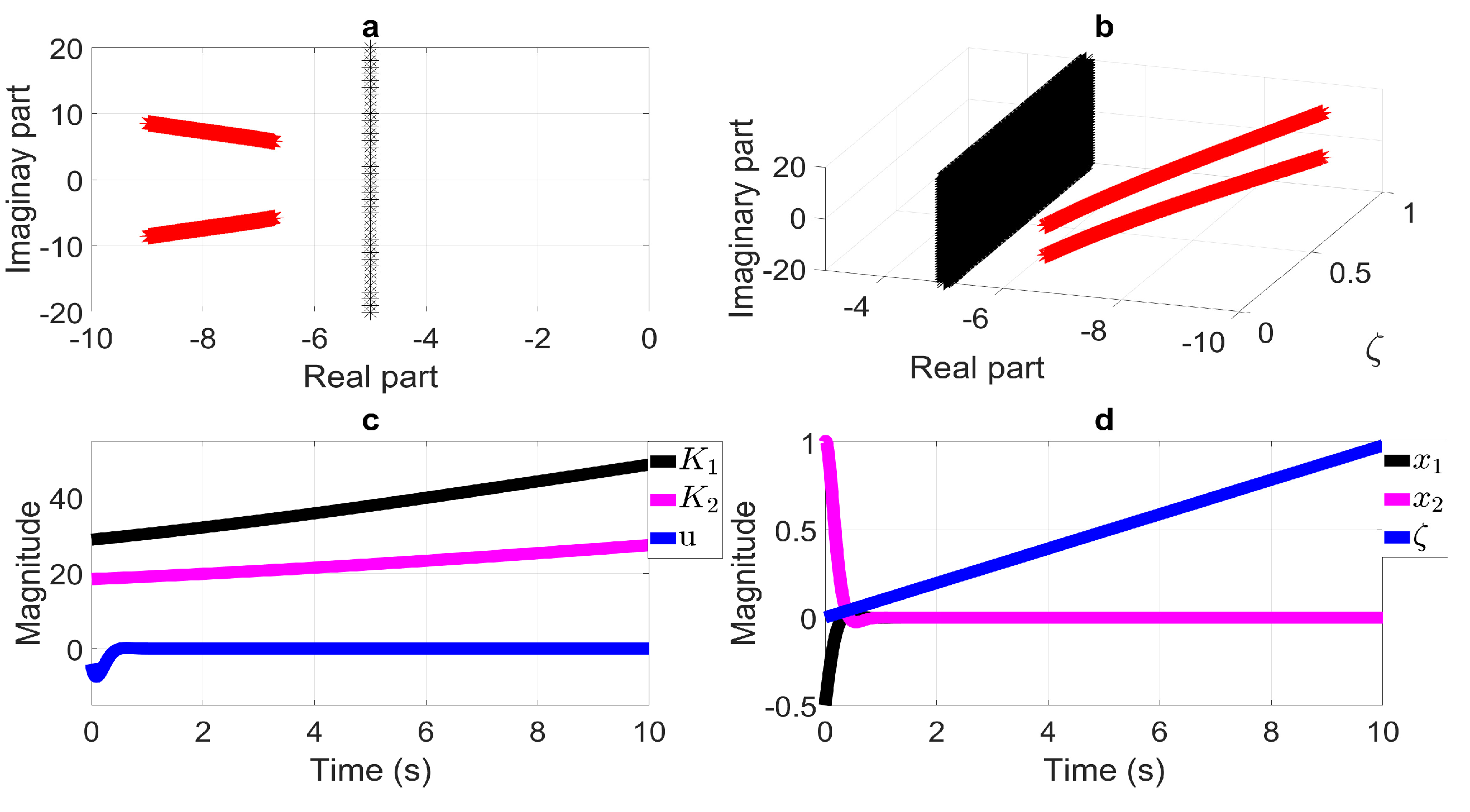
6.1. Half-Plane LMI Region

The half-plane LMI region aims at placing eigenvalues on the left side of a desired value, i.e., $Re\left(z\right)<-\alpha$, with characteristic function:

$$f_D\left(z\right)=2\alpha +z+\overline{z}.$$

(35)

In addressing this result, let us point out that from Equation (14), by considering Equation (18), straightforward calculations result in:

$$\begin{array}{c}2\alpha (\overline{Q}\left(\zeta \right)-\dot{\zeta }({\overline{Q}}_1+2{\overline{Q}}_2\zeta ))+\sum _{i=0}^4{\alpha }_i{\zeta }^i+\sum _{i=0}^4{\left({\alpha }_i\right)}^{\top }{\zeta }^i⩽0\Rightarrow \\ 2\alpha ({\overline{Q}}_0-{\overline{Q}}_1\dot{\zeta })+2\alpha ({\overline{Q}}_1-2{\overline{Q}}_2\dot{\zeta })\zeta +2\alpha {\overline{Q}}_2{\zeta }^2+\sum _{i=0}^4{\alpha }_i{\zeta }^i+\sum _{i=0}^4{\left({\alpha }_i\right)}^{\top }{\zeta }^i⩽0,\end{array}$$

(36)

which is equivalent to

$$\sum _{i=0}^4{N}_j{\zeta }^j⩽0,$$

(37)

with:

$$\begin{array}{c}{N}_0=2\alpha {\overline{Q}}_0-2\alpha {\overline{Q}}_1\dot{\zeta }+{\alpha }_0+{\alpha }_0^{\top },N_1=2\alpha {\overline{Q}}_1-4\alpha {\overline{Q}}_2\dot{\zeta }+{\alpha }_1+{\alpha }_1^{\top },\\ N_2=2\alpha {\overline{Q}}_2+{\alpha }_2+{\alpha }_2^{\top },N_3={\alpha }_3+{\alpha }_3^{\top },N_4={\alpha }_4+{\alpha }_4^{\top }.\end{array}$$

Let us point out that, finally, Equations (36) and (37) are Equation (19) with $\zeta =\beta$. From this, notice that Proposition 1 can be applied. By considering $\dot{\zeta }=0.1$ and $\alpha =5$ along with Yalmip [37] and Sedumi [38] within Matlab, the following results are found:

$$\begin{array}{c}\begin{array}{c}\overline{Q}\left(\zeta \right)={\overline{Q}}_0+{\overline{Q}}_1\zeta +{\overline{Q}}_2{\zeta }^2\\ =\left[\begin{array}{cc}0.416& -0.941\\ ★& 3.092\end{array}\right]+\left[\begin{array}{cc}0.152& -0.336\\ ★& 0.869\end{array}\right]\zeta +\left[\begin{array}{cc}0.034& -0.031\\ ★& 0.041\end{array}\right]{\zeta }^2,\end{array}\end{array}$$

$$r2=0.144,r3=0.038,r4=0.028,s=1.318,$$

$$\begin{array}{c}\overline{K}\left(\zeta \right)={\overline{K}}_0+{\overline{K}}_1\zeta +{\overline{K}}_2{\zeta }^2,\\ =\begin{array}{c}\left[\begin{array}{c}-5.34329.798\end{array}\right]+\left[\begin{array}{c}-1.53511.861\end{array}\right]\zeta +\left[\begin{array}{c}0.3394.543\end{array}\right]{\zeta }^2.\end{array}\end{array}$$

As a result, Proposition 1 is accomplished, with these results giving rise to a continuous control gain at a specific value for $\zeta$ defined by:

$$K\left(\zeta \right)=\overline{K}\left(\zeta \right){\left[\overline{Q}\left(\zeta \right)\right]}^{-1}.$$

(38)

Figure 2 shows the results for this LMI region.

From Figure 2a, it is possible to see the closed-loop eigenvalues’ allocation to the left side of $\alpha =-5$ in the half-plane. Figure 2b, in turn, shows the real and imaginary parts of the closed-loop eigenvalues as a function of the time-varying parameter while it is moving from 0 to 1. Figure 2c,d, finally, show the control gain and control law and the system state from an initial condition ${[-0.51]}^{\top }$ and time-varying parameter variation, respectively. From Figure 2, the accurate results for this LMI region can be clearly viewed. Let us point out that the feasibility of Proposition 1 will depend on the time-varying parameter inference in the system, from the fact that a stronger parameter(s)’s influence within the system could generate a complexity increment for the LMI solver, giving rise to inaccurate or nonfeasible results. From a practical point of view, on the other hand, as long as the time-varying parameter is measured, notice that it will be used in the control gain computation once the solver has found the overall solution. With this, finally, it is possible to conclude that the control gain computation depends in general on the LPV system in terms of $\zeta$, viewed from the solver considered for computing Proposition 1’s results.

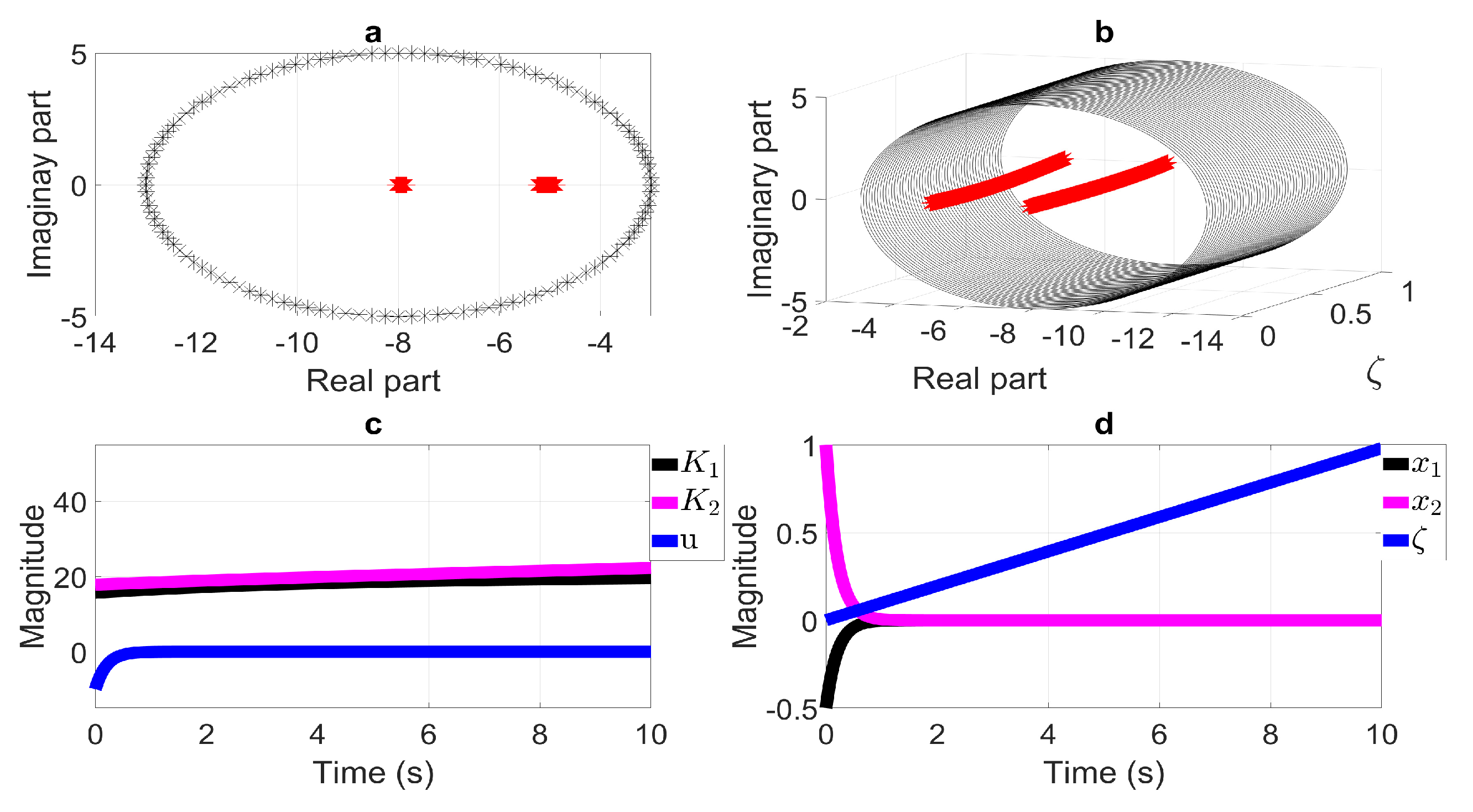
6.2. Disk LMI Region

The disk LMI region aims at placing the closed eigenvalues within a disk of radius r centered in q, specified by the following:

$$f_D\left(z\right)=\left[\begin{array}{cc}-r& z+q\\ \overline{z}+q& -r\end{array}\right].$$

(39)

Again, let us point out from Equation (14) that:

$$\left[\begin{array}{cc}-r(\overline{Q}\left(\zeta \right)-\dot{\zeta }({\overline{Q}}_1+2{\overline{Q}}_2\zeta ))& q(\overline{Q}\left(\zeta \right)-\dot{\zeta }({\overline{Q}}_1+2{\overline{Q}}_2\zeta ))+\sum _{i=0}^4{\alpha }_i{\zeta }^i\\ q(\overline{Q}\left(\zeta \right)-\dot{\zeta }({\overline{Q}}_1+2{\overline{Q}}_2\zeta ))+\sum _{i=0}^4{\alpha }_i^{\top }{\zeta }^i& -r(\overline{Q}\left(\zeta \right)-\dot{\zeta }({\overline{Q}}_1+2{\overline{Q}}_2\zeta ))\end{array}\right]⩽0.$$

(40)

Let us consider Equation (40) as:

$$\left[\begin{array}{cc}{\Omega }_{1,1}& {\Omega }_{1,2}\\ {\Omega }_{2,1}& {\Omega }_{2,2}\end{array}\right]⩽0,$$

(41)

with:

$$\begin{array}{c}{\Omega }_{1,1}=-r({\overline{Q}}_0-\dot{\zeta }{\overline{Q}}_1)-r({\overline{Q}}_1-2\dot{\zeta }{\overline{Q}}_2)\zeta -r{\overline{Q}}_2{\zeta }^2\hfill \\ {\Omega }_{1,2}={\alpha }_0+q({\overline{Q}}_0-\dot{\zeta }{\overline{Q}}_1)+\left[q({\overline{Q}}_1-2\dot{\zeta }{\overline{Q}}_2)+{\alpha }_1\right]\zeta +(q{\overline{Q}}_2+{\alpha }_2){\zeta }^2+{\alpha }_3{\zeta }^3+{\alpha }_4{\zeta }^4\hfill \\ {\Omega }_{2,1}={\alpha }_0^{\top }+q({\overline{Q}}_0-\dot{\zeta }{\overline{Q}}_1)+\left[q({\overline{Q}}_1-2\dot{\zeta }{\overline{Q}}_2)+{\alpha }_1^{\top })\right]\zeta +(q{\overline{Q}}_2+{\alpha }_2^{\top }){\zeta }^2+{\alpha }_3^{\top }{\zeta }^3+{\alpha }_4^{\top }{\zeta }^4\hfill \\ {\Omega }_{2,2}={\Omega }_{1,1}.\hfill \end{array}$$

Further, notice that Equation (41), derived from Equation (40) with Equation (18), can be presented in matrix form by gathering its elements in terms of $\zeta$ as follows:

$$\sum _{i=0}^4{N}_j{\zeta }^j⩽0,$$

(42)

by considering:

$$\begin{array}{c}{N}_0=\left[\begin{array}{cc}-r({\overline{Q}}_0-\dot{\zeta }{\overline{Q}}_1)& q({\overline{Q}}_0-\dot{\zeta }{\overline{Q}}_1)+{\alpha }_0\\ q({\overline{Q}}_0-\dot{\zeta }{\overline{Q}}_1)+{\alpha }_0^{\top }& -r({\overline{Q}}_0-\dot{\zeta }{\overline{Q}}_1)\end{array}\right]\hfill \\ N_1=\left[\begin{array}{cc}-r({\overline{Q}}_1-2\dot{\zeta }{\overline{Q}}_2)& q({\overline{Q}}_1-2\dot{\zeta }{\overline{Q}}_2)+{\alpha }_1\\ q({\overline{Q}}_1-2\dot{\zeta }{\overline{Q}}_2)+{\alpha }_1^{\top }& -r({\overline{Q}}_1-2\dot{\zeta }{\overline{Q}}_2)\end{array}\right]\hfill \\ N_2=\left[\begin{array}{cc}-r{\overline{Q}}_2& q{\overline{Q}}_2+{\alpha }_2\\ q{\overline{Q}}_2+{\alpha }_2^{\top }& -r{\overline{Q}}_2\end{array}\right],N_3=\left[\begin{array}{cc}0& {\alpha }_3\\ {\alpha }_3^{\top }& 0\end{array}\right],N_4=\left[\begin{array}{cc}0& {\alpha }_4\\ {\alpha }_4^{\top }& 0\end{array}\right].\hfill \end{array}$$

As a consequence, finally, Equation (42) is Equation (19) with $\zeta =\beta$, and Proposition 1 can be applied. For this test, similar initial conditions for the system state, parameter $\dot{\zeta }$, and the software for the computation of the results are considered as in the previous LMI region. Recall that ${\alpha }_1$, $i=1,2,\dots ,4$, is taken from Equation (19). By selecting $q=8$ and $r=5$, the following are computed:

$$\begin{array}{c}\begin{array}{c}\overline{Q}\left(\zeta \right)={\overline{Q}}_0+{\overline{Q}}_1\zeta +{\overline{Q}}_2{\zeta }^2\\ =\left[\begin{array}{cc}0.09& -0.178\\ ★& 0.411\end{array}\right]+\left[\begin{array}{cc}0.038& -0.062\\ ★& 0.113\end{array}\right]\zeta +\left[\begin{array}{cc}0.025& -0.035\\ ★& 0.057\end{array}\right]{\zeta }^2\end{array}\end{array}$$

$$r2=0.012,r3=0.007,r4=0.004,s=1.367$$

$$\begin{array}{c}\begin{array}{c}\overline{K}\left(\zeta \right)={\overline{K}}_0+{\overline{K}}_1\zeta +{\overline{K}}_2{\zeta }^2\\ =\left[\begin{array}{c}-1.774.535\end{array}\right]+\left[\begin{array}{c}-0.7011.758\end{array}\right]\zeta +\left[\begin{array}{c}-0.6781.3\end{array}\right]{\zeta }^2.\end{array}\end{array}$$

Notice Proposition 1’s accomplishment, with these results giving rise to the presented Figure 3. Finally, the continuous control gain will be computed as in Equation (38).

From Figure 3a, one can see the closed-loop eigenvalues allocated within the disk centered at 8 with radius 5 in the left subset of the complex plane. In turn, Figure 3b shows the eigenvalues’ real and imaginary part allocation as a function of the time-varying parameter while it is moving from 0 to 1. Figure 3c,d, finally, show the control gain and control law and the system states and time-varying parameter variation, respectively.

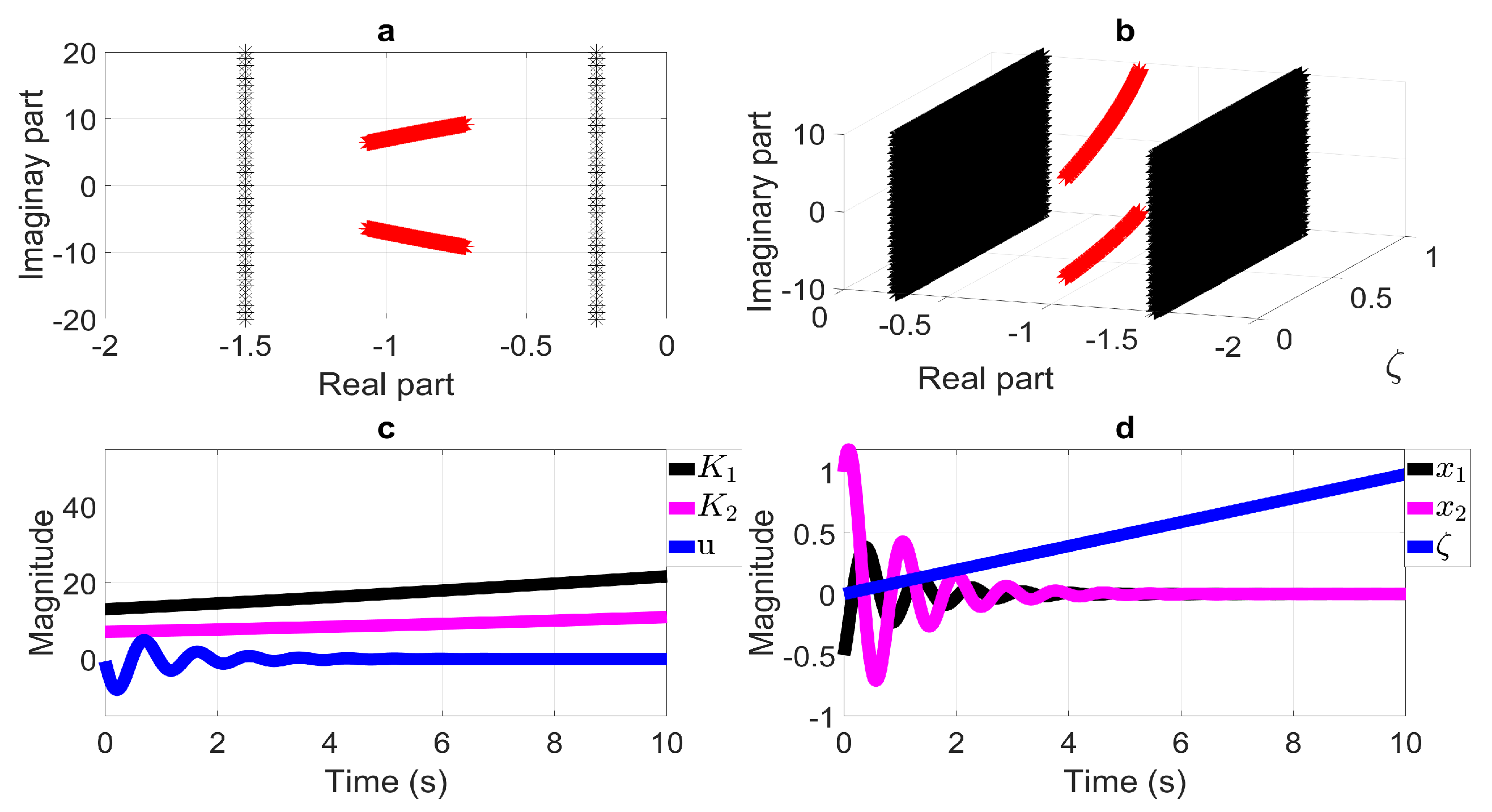
6.3. Vertical Bands LMI Region

As for the vertical bands LMI region, notice the complex-plane function defined as:

$$f_D\left(z\right)=\left[\begin{array}{cc}2a_1+z+\overline{z}& 0\\ 0& -2a_2-z-\overline{z}\end{array}\right],$$

(43)

aiming at placing the closed-loop eigenvalues within the complex plane region defined by parameters $a_1$ and $a_2$. With this, the following from Equations (14) and (18) can be computed:

$$\begin{array}{c}\left[\begin{array}{c}2a_1(\overline{Q}\left(\zeta \right)-\dot{\zeta }({\overline{Q}}_1+2{\overline{Q}}_2\zeta )+\sum _{i=0}^4{\alpha }_i{\zeta }^i+\sum _{i=0}^4{\alpha }_i^{\top }{\zeta }^i\\ 0\end{array}\right.\\ \left.\begin{array}{c}0\\ -2a_2(\overline{Q}\left(\zeta \right)-\dot{\zeta }({\overline{Q}}_1+2{\overline{Q}}_2\zeta )-\sum _{i=0}^4{\alpha }_i{\zeta }^i-\sum _{i=0}^4{\alpha }_i^{\top }{\zeta }^i\end{array}\right]\end{array}⩽0,$$

(44)

where the second line of Equation (44) corresponds to the elements of the second column of Equation (43). Notice that the corresponding expansion of Equation (44), gathering its elements in terms of $\zeta$, can be represented as:

$$\sum _{i=0}^4{N}_j{\zeta }^j⩽0,$$

(45)

with:

$$\begin{array}{c}{N}_0=\left[\begin{array}{cc}{N}_{01}& 0\\ 0& N_{04}\end{array}\right],N_1=\left[\begin{array}{cc}{N}_{11}& 0\\ 0& N_{14}\end{array}\right],\hfill \\ N_2=\left[\begin{array}{cc}2a_1{\overline{Q}}_2+{\alpha }_2+{\alpha }_2^{\top }& 0\\ 0& -2a_2{\overline{Q}}_2-{\alpha }_2-{\alpha }_2^{\top }\end{array}\right]\hfill \\ N_3=\left[\begin{array}{cc}{\alpha }_3+{\alpha }_3^{\top }& 0\\ 0& -{\alpha }_3-{\alpha }_3^{\top }\end{array}\right],N_4=\left[\begin{array}{cc}{\alpha }_4+{\alpha }_4^{\top }& 0\\ 0& -{\alpha }_4+{\alpha }_4^{\top }\end{array}\right],\hfill \end{array}$$

considering $N_{01}=2a_1({\overline{Q}}_0-\dot{\zeta }{\overline{Q}}_1)+{\alpha }_0+{\alpha }_0^{\top }$, $N_{04}=-2a_2({\overline{Q}}_0-\dot{\zeta }{\overline{Q}}_1)-{\alpha }_0-{\alpha }_0^{\top }$, $N_{11}=2a_1({\overline{Q}}_1-2\dot{\zeta }{\overline{Q}}_2)+{\alpha }_1+{\alpha }_1^{\top }$ and $N_{14}=-2a_2({\overline{Q}}_1-2\dot{\zeta }{\overline{Q}}_2)-{\alpha }_1-{\alpha }_1^{\top }$.

Focusing on Equation (45), the expression is, now again, as in Equation (19) with $\zeta =\beta$. As a consequence, Proposition 1 can be applied. For this LMI region, parameters $a_1=0.25$ and $a_2=1.5$ were selected by considering initial conditions for the system state and parameter $\dot{\zeta }$ as in the previous test. The results for this LMI region are depicted in Figure 4, with similar interpretations as in previous results and decision variables computed as:

$$\begin{array}{c}\begin{array}{c}\overline{Q}\left(\zeta \right)={\overline{Q}}_0+{\overline{Q}}_1\zeta +{\overline{Q}}_2{\zeta }^2\\ =\left[\begin{array}{cc}0.183& -0.138\\ ★& 0.935\end{array}\right]+\left[\begin{array}{cc}0.018& -0.029\\ ★& 0.071\end{array}\right]\zeta +\left[\begin{array}{cc}0.009& -0.01\\ ★& 0.017\end{array}\right]{\zeta }^2\end{array}\end{array}$$

$$r2=0.018,r3=0.008,r4=0.008,s=2.216$$

$$\begin{array}{c}\overline{K}\left(\zeta \right)={\overline{K}}_0+{\overline{K}}_1\zeta +{\overline{K}}_2{\zeta }^2\\ =\left[\begin{array}{c}1.44.87\end{array}\right]+\left[\begin{array}{c}0.9851.891\end{array}\right]\zeta +\left[\begin{array}{c}0.2390.698\end{array}\right]{\zeta }^2\end{array}$$

Notice Proposition 1 is accomplished, giving rise to the closed-loop eigenvalues’ allocation within the addressed LMI region.

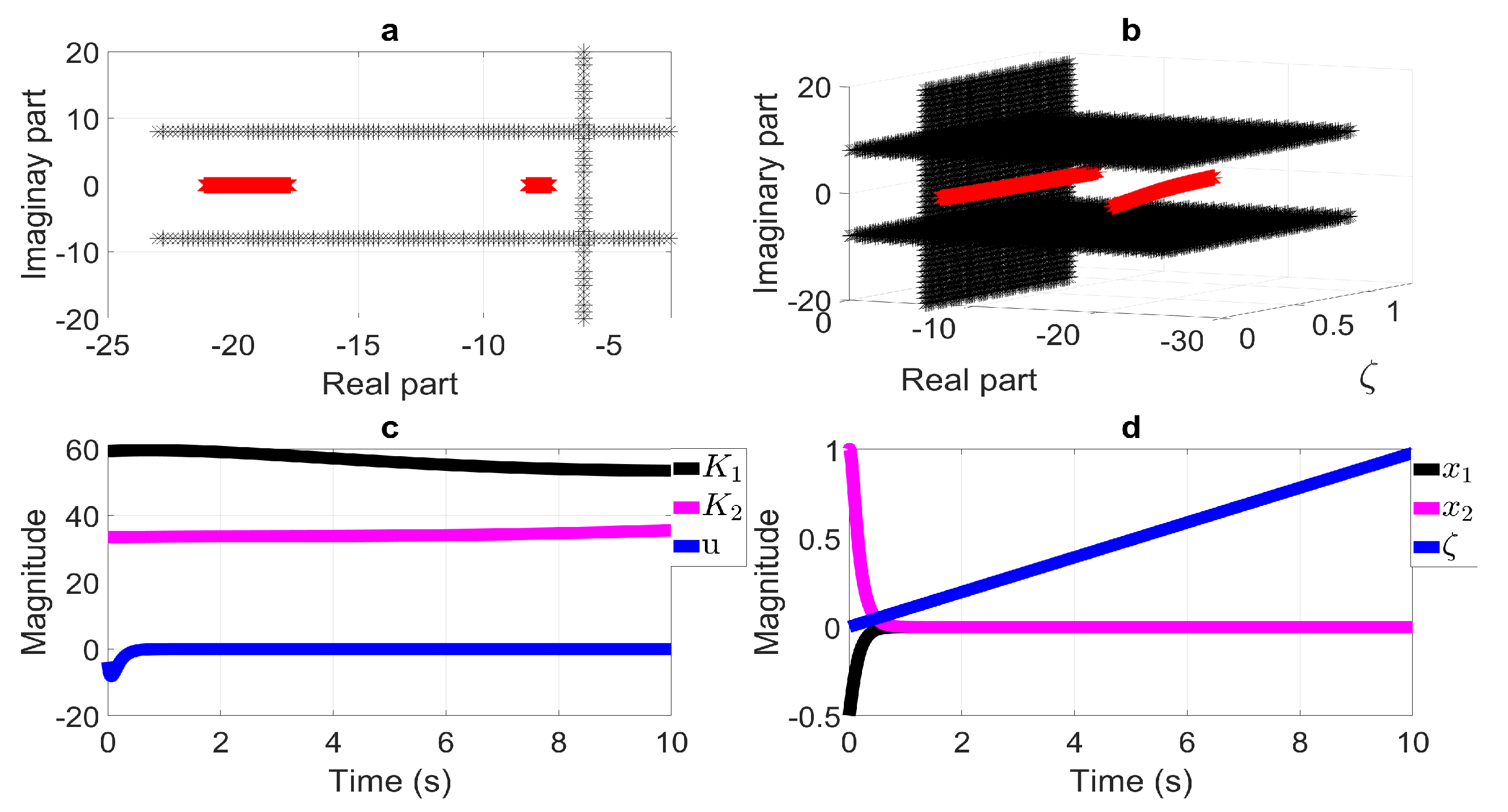
6.4. LMI Region Intersection: Horizontal Half-Strip and Half-Plane LMI Region

As an additional result aiming at showing the effectiveness of the proposed method, let us focus on an LMI region intersection. The objective here is to place the closed-loop eigenvalues from a controller design within a complex-plane region defined by two LMI regions. For this, let us focus on the horizontal half-strip LMI region defined by:

$$f_D\left(z\right)=\left[\begin{array}{cc}-2\sigma & z-\overline{z}\\ -z+\overline{z}& -2\sigma \end{array}\right],$$

(46)

where $\sigma$ represents the magnitude of the limit associated with the horizontal strip. This, in turn, can be represented in terms of the closed-loop system as follows:

$$\left[\begin{array}{cc}{\Gamma }_1& {\Gamma }_2\\ -{\Gamma }_2& {\Gamma }_1\end{array}\right]⩽0,$$

(47)

with:

$$\begin{array}{ccc}{\Gamma }_1& =& -2\sigma \left[{\overline{Q}}_0+{\overline{Q}}_1\zeta +{\overline{Q}}_2{\zeta }^2-\dot{\zeta }({\overline{Q}}_1-2{\overline{Q}}_2\zeta )\right]\hfill \\ & =& -2\sigma ({\overline{Q}}_0-{\overline{Q}}_1\dot{\zeta })-2\sigma ({\overline{Q}}_1+2\dot{\zeta }{\overline{Q}}_2)\zeta -2\sigma {\overline{Q}}_2{\zeta }^2\hfill \\ {\Gamma }_2& =& \sum _{i=0}^4{\alpha }_i{\zeta }^i-\sum _{i=0}^4{\alpha }_i^{\top }{\zeta }^i,\hfill \end{array}$$

giving rise to Equation (19) with $\beta =\zeta$ and:

$$\begin{array}{c}{N}_0=\left[\begin{array}{cc}-2\sigma ({\overline{Q}}_0-{\overline{Q}}_1\dot{\zeta })& {\alpha }_0-{\alpha }_0^{\top }\\ -{\alpha }_0+{\alpha }_0^{\top }& -2\sigma ({\overline{Q}}_0-{\overline{Q}}_1\dot{\zeta })\end{array}\right]\hfill \\ N_1=\left[\begin{array}{cc}-2\sigma ({\overline{Q}}_1+2\dot{\zeta }{\overline{Q}}_2)& {\alpha }_1-{\alpha }_1^{\top }\\ -{\alpha }_1+{\alpha }_1^{\top }& -2\sigma ({\overline{Q}}_1+2\dot{\zeta }{\overline{Q}}_2)\end{array}\right]\hfill \\ N_2=\left[\begin{array}{cc}-2\sigma {\overline{Q}}_2& {\alpha }_2-{\alpha }_2^{\top }\\ -{\alpha }_2+{\alpha }_2^{\top }& -2\sigma {\overline{Q}}_2\end{array}\right],N_3=\left[\begin{array}{cc}0& {\alpha }_3-{\alpha }_3^{\top }\\ -{\alpha }_3+{\alpha }_3^{\top }& 0\end{array}\right]\hfill \\ N_4=\left[\begin{array}{cc}0& {\alpha }_4-{\alpha }_4^{\top }\\ -{\alpha }_4+{\alpha }_4^{\top }& 0\end{array}\right].\hfill \end{array}$$

Notice that this LMI region intersection is accomplished by gathering a horizontal half-strip with $\sigma =8$ and a half-plane LMI region with $\alpha =6$ (as in Section 6.1), by maintaining the same decision variables in common. The computed results are found to be:

$$\begin{array}{c}\begin{array}{c}\overline{Q}\left(\zeta \right)={\overline{Q}}_0+{\overline{Q}}_1\zeta +{\overline{Q}}_2{\zeta }^2\\ =\left[\begin{array}{cc}0.017& -0.043\\ ★& 0.14\end{array}\right]+\left[\begin{array}{cc}0.025& -0.053\\ ★& 0.12\end{array}\right]\zeta +\left[\begin{array}{cc}0.016& -0.021\\ ★& 0.027\end{array}\right]{\zeta }^2\end{array}\end{array}$$

$$r2=0.016,r3=0.005,r4=0.002,s=1.32$$

$$\begin{array}{c}\begin{array}{c}\overline{K}\left(\zeta \right)={\overline{K}}_0+{\overline{K}}_1\zeta +{\overline{K}}_2{\zeta }^2\\ =\left[\begin{array}{c}-0.4152.187\end{array}\right]+\left[\begin{array}{c}-0.2660.8824\end{array}\right]\zeta +\left[\begin{array}{c}-0.3240.9316\end{array}\right]{\zeta }^2.\end{array}\end{array}$$

Recall that those LMI regions considered within the intersection must be solved simultaneously by maintaining common decision variables. The results of this LMI region intersection are depicted in Figure 5.

From Figure 5a, one can see the closed-loop eigenvalues allocated within the complex plane region defined by parameters $\sigma$ and $\alpha$. In turn, Figure 5b shows the eigenvalues’ real and imaginary parts’ allocation as a function of the time-varying parameter, varying from 0 to 1. Figure 5c,d, finally, show the control gain and control law and the system states and time-varying parameter variation, respectively. From Figure 5, the accurate results for this LMI region’s intersection can be clearly perceived.

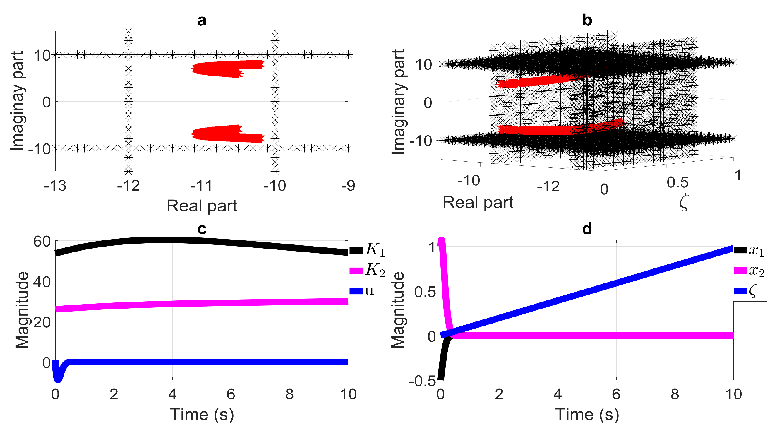
6.5. LMI Region Intersection: Horizontal Half-Strip and Vertical Bands LMI Region

For this result, the intersection between a horizontal half-strip and vertical bands’ LMI regions are considered. This is accomplished by gathering Equation (47) and that presented in Section 6.3, by maintaining the same decision variables in common. Considering parameters defining LMI regions $a_1=10$ and $a_2=12$ and $\sigma =10$, the computed results are found to be:

$$\begin{array}{c}\begin{array}{c}\overline{Q}\left(\zeta \right)={\overline{Q}}_0+{\overline{Q}}_1\zeta +{\overline{Q}}_2{\zeta }^2\\ =\left[\begin{array}{cc}0.011& -0.043\\ ★& 0.207\end{array}\right]+\left[\begin{array}{cc}0.004& -0.010\\ ★& 0.03\end{array}\right]\zeta +\left[\begin{array}{cc}0.006& -0.008\\ ★& 0.016\end{array}\right]{\zeta }^2\end{array}\end{array}$$

$$r2=0.0059,r3=0.0026,r4=0.0013,s=1.2349$$

$$\begin{array}{c}\begin{array}{c}\overline{K}\left(\zeta \right)={\overline{K}}_0+{\overline{K}}_1\zeta +{\overline{K}}_2{\zeta }^2\\ =\left[\begin{array}{c}-0.4993.072\end{array}\right]+\left[\begin{array}{c}-0.040.751\end{array}\right]\zeta +\left[\begin{array}{c}-0.1570.431\end{array}\right]{\zeta }^2,\end{array}\end{array}$$

with the corresponding results depicted in Figure 6 and the interpretation as in previous results.

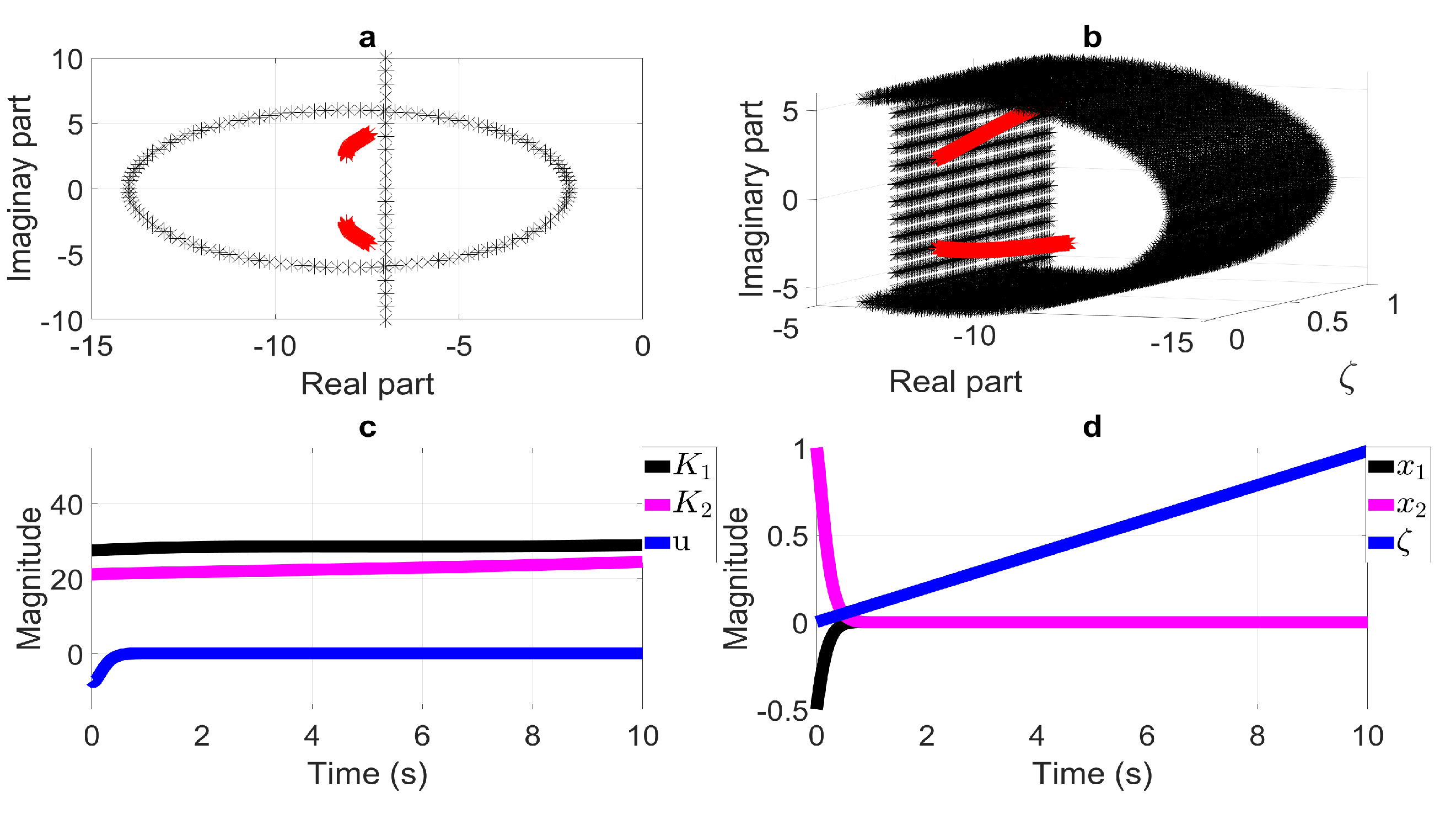
6.6. LMI Region Intersection: Disk LMI Region and Half-Plane LMI Region

As a final result, an LMI region intersection from a disk and half-plane is presented. For this, the procedure shown in Section 6.1 and Section 6.2 is considered by applying the same characteristic at the solution level mentioned in the previous LMI region intersections. A disk with radius $r=6$ centered at $q=7$ and $\alpha =7$ was considered, giving rise to the following results:

$$\begin{array}{c}\begin{array}{c}\overline{Q}\left(\zeta \right)={\overline{Q}}_0+{\overline{Q}}_1\zeta +{\overline{Q}}_2{\zeta }^2\\ =\left[\begin{array}{cc}0.063& -0.168\\ ★& 0.513\end{array}\right]+\left[\begin{array}{cc}0.034& -0.064\\ ★& 0.127\end{array}\right]\zeta +\left[\begin{array}{cc}0.021& -0.028\\ ★& 0.038\end{array}\right]{\zeta }^2\end{array}\end{array}$$

$$r2=0.012,r3=0.004,r4=0.002,s=1.574$$

$$\begin{array}{c}\begin{array}{c}\overline{K}\left(\zeta \right)={\overline{K}}_0+{\overline{K}}_1\zeta +{\overline{K}}_2{\zeta }^2\\ =\left[\begin{array}{c}-1.8246.23\end{array}\right]+\left[\begin{array}{c}-0.6061.713\end{array}\right]\zeta +\left[\begin{array}{c}-0.5021.171\end{array}\right]{\zeta }^2\end{array}\end{array}$$

Notice that Figure 7 has the same interpretation as in previous cases. Finally, from the presented results, it is possible to conclude that the proposed procedure is applicable, with accurate performance, to several LMI regions and intersections between them. In conclusion, as long as the solver is able to compute the solution for the closed-loop system considering combinations of different LMIs, the corresponding eigenvalues will lie in the resulting LMI region composed of those originally desired.

7. Remarks

From the presented results, it is important for the reader to understand the following remarks, mainly referring to higher-order time-varying dependency and LMI regions applied to PLPV systems.

• On higher-order time-varying dependency with respect to the considered application example.
  It is important to explain the application of the procedure presented throughout this paper in the case of having higher time-varying parameter dependency with respect to that presented in Section 6, i.e., in the case of $k>2$ in Equation (2). If that is the case, with $k=4$ in Equation (2) as an example, notice that the system matrix will be:

  $$A\left(\zeta \right)=A_0+A_1\zeta +A_2{\zeta }^2+A_3{\zeta }^3+A_4{\zeta }^4,$$

  (48)

  giving rise to, for the controller design, $\overline{Q}\left(\zeta \right)$ and $\overline{K}\left(\zeta \right)$ with the same order. As a consequence, a closed-loop system with a generalized form can be defined as:

  $$\sum _{i=0}^8{\alpha }_i{\zeta }^i+\sum _{i=0}^8{\left({\alpha }_i\right)}^{\top }{\zeta }^i-\dot{\zeta }({\overline{Q}}_1+2{\overline{Q}}_2\zeta +3{\overline{Q}}_3{\zeta }^2+4{\overline{Q}}_4{\zeta }^3)<0,$$

  (49)

  resulting in a higher time-varying dependency in the PLMI: a summary of nine elements. This particular case implies the need to apply the DC convexification method presented in Section 5.2 twice, from the resulting PLMI described in Equation (19), and, finally, both LMIs should be solved simultaneously from Proposition 1. In general terms, the DC convexification method allows us to perform a PLMI relaxation, aiming at its computation by applying a set of defined lemmas [31]. As a result, a generalized procedure from that presented throughout this paper can be defined from the system dependency on the time-varying parameter, after having a closed-loop system with a continuous control gain and the desired LMI region. From this, depending on the PLMI’s structure, the corresponding lemma will be needed within the proposed procedure, aiming at performing the PLMI relaxation and, as a result, the state-feedback control gain computation.
• In the case of having time-varying parameter dependency on matrix B.
  Additionally to that previously presented, let us focus on the case of having time-varying parameter dependency on the B matrix from that considered within this paper, with generalized form:

  $$B\left(\zeta \right)=B_0+B_1\zeta +B_2{\zeta }^2.$$

  (50)
  The issue is related to this implication within the previously shown procedure. In addressing this case, notice the Lyapunov stability theory’s application to PLPV systems:

  $$A\left(\zeta \right)\overline{Q}\left(\zeta \right)-B\left(\zeta \right)\overline{K}\left(\zeta \right)+\overline{Q}{\left(\zeta \right)}^{\top }A{\left(\zeta \right)}^{\top }-\overline{K}{\left(\zeta \right)}^{\top }B{\left(\zeta \right)}^{\top }-\dot{\zeta }\frac{\partial \overline{Q}\left(\zeta \right)}{\partial \zeta }<0,$$

  (51)

  considering Equations (16) and (50) will lie in:

  $$\begin{array}{c}(A_0+A_1\zeta +A_2{\zeta }^2)({\overline{Q}}_0+{\overline{Q}}_1\zeta +{\overline{Q}}_2{\zeta }^2)-(B_0+B_1\zeta +B_2{\zeta }^2)({\overline{K}}_0+{\overline{K}}_1\zeta +{\overline{K}}_2{\zeta }^2)+\\ {({\overline{Q}}_0+{\overline{Q}}_1\zeta +{\overline{Q}}_2{\zeta }^2)}^{\top }{(A_0+A_1\zeta +A_2{\zeta }^2)}^{\top }-\\ {({\overline{K}}_0+{\overline{K}}_1\zeta +{\overline{K}}_2{\zeta }^2)}^{\top }{(B_0+B_1\zeta +B_2{\zeta }^2)}^{\top }-\dot{\zeta }\frac{\partial \left({\overline{Q}}_0+{\overline{Q}}_1\zeta +{\overline{Q}}_2{\zeta }^2\right)}{\partial \zeta }<0,\end{array}$$

  (52)

  which in turn can be generalized as:

  $$\sum _{i=0}^4{\alpha }_i{\zeta }^i+\sum _{i=0}^4{\left({\alpha }_i\right)}^{\top }{\zeta }^i-\dot{\zeta }({\overline{Q}}_1+2{\overline{Q}}_2\zeta )<0,$$

  (53)

  with:

  $$\begin{array}{c}{\alpha }_0=A_0{\overline{Q}}_0-B_0{\overline{K}}_0\\ {\alpha }_1=A_0{\overline{Q}}_1-B_0{\overline{K}}_1+A_1{\overline{Q}}_0-B_1{\overline{K}}_0\\ {\alpha }_2=A_0{\overline{Q}}_2-B_0{\overline{K}}_2+A_1{\overline{Q}}_1-B_1{\overline{K}}_1+A_2{\overline{Q}}_0-B_2{\overline{K}}_0\\ {\alpha }_3=A_1{\overline{Q}}_2-B_1{\overline{K}}_2+A_2{\overline{Q}}_1-B_2{\overline{K}}_1\\ {\alpha }_4=A_2{\overline{Q}}_2-B_2{\overline{K}}_2\end{array}$$
  From Equation (53), one can perceive similar conditions as those presented in the controller design section (Section 5.1), i.e., as those from which the PLMI relaxation procedure begins (see Section 5.2). As a result, the B matrix with time-varying dependence through $\zeta$ does not affect the development presented throughout this paper in terms of LMI regions.
• On the LMI region’s definition and its application to PLPV systems.
  To explain the use of LMI regions in PLPV systems from the procedure shown throughout this paper, let us point out that there are some LMI regions excluded by means of the presented method. The previous is important due to the fact that some LMI regions characterized by a function of complex plane $f_D\left(z\right)$ which excludes the substitution of the first term on its representation should not be considered (conic LMI regions, for instance). For this, let us focus on Equation (14) in Section 4, defining a stable matrix if $M_D(A\left(\zeta \right),Q\left(\zeta \right))<0$, with $Q\left(\zeta \right)=Q{\left(\zeta \right)}^{\top }$ (see Section 3.1). To ensure the closed-loop eigenvalues lie in a specific subset of the complex plane defined by $f_D\left(z\right)$ through a state-feedback controller, LMI regions should contain the first term related to substitution $1=X\left(\zeta \right)$, $z=\left(A\right(\zeta \left)X\right(\zeta \left)\right)$ and $\overline{z}={\left(A\left(\zeta \right)X\left(\zeta \right)\right)}^{\top }$, i.e., as an example, $2\alpha (\overline{Q}\left(\zeta \right)-\dot{\zeta }({\overline{Q}}_1+2{\overline{Q}}_2\zeta ))$ defines a half-plane LMI region. The reason for this comes from the fact that the mentioned substitution ensures a closed-loop system by considering the main characteristic of a PLVP system, the rate of the time-varying parameter ($\dot{\zeta }$) as a tuning controller parameter.
• In the case of having the system affected by model uncertainties.
  An important issue related to applying the controller design method presented in this paper is the case of the system being affected by modeling uncertainties. Notice that such considerations would require additional elements in the structure of the control system to face these particularities at the design level. Let us point out that, if this is the case, additional analyses must be carried out to generate variations of the proposed method, thereby achieving a control system with continuous control gain that considers the time-varying parameter rate as a tuning parameter and LMI regions within the design.

8. Conclusions

The present paper addresses LMI regions applied to linear parameter-varying (LPV) systems with high-order time-varying dependency, named polynomial LPV systems. Throughout this paper, a procedure for ensuring that closed-loop eigenvalues with a state-feedback control lie in a subset of the complex plane has been presented, viewed as an extension of LMI regions applied to linear time-invariant systems towards polynomial LPV systems and considered as the main contribution of the present paper. In this contribution, the computed state-feedback control gain is obtained continuously from a parameterized linear matrix inequality relaxation by taking into account the time-varying parameter rate as a tuning parameter within the controller design. A remark section includes important issues to be considered before applying the presented method, aiming at presenting considerations within the procedure shown in the paper. Finally, from the presented results, the effectiveness of the proposed method can be concluded, including, inclusively, LMI region intersections.

References

1. Shamma, J.S. An Overview of LPV Systems. In Control of Linear Parameter Varying Systems with Applications, 1st ed.; Springer: Boston, MA, USA, 2012. [Google Scholar]
2. López-Estrada, F.R.; Rotondo, D.; Valencia-Palomo, G. A Review of Convex Approaches for Control, Observation and Safety of Linear Parameter Varying and Takagi-Sugeno Systems. Process 2019, 7, 814. [Google Scholar] [CrossRef]
3. Tóth, R. Modeling and Identification of Linear Parameter-Varying Systems, 1st ed.; Springer: Berlin/Heidelberg, Germany, 2010. [Google Scholar]
4. McCloy, R.; Li, Y.; Bao, J.; Skyllas-Kazacos, M. Electrolyte flow rate control for vanadium redox flow batteries using the linear parameter varying framework. J. Process Control 2022, 115, 36–47. [Google Scholar] [CrossRef]
5. Fuentes, R.M.; Palma, J.M.; Júnior, H.G.; Lacerda, M.J.; Carvalho, L.d.P.; Rojas, A.J.; Oliveira, R.C.L.F. Gain-Scheduled Control Design Applied to Classical dc-dc Converters in Photovoltaic Systems and Constant Power Loads. Mathematics 2022, 10, 3467. [Google Scholar] [CrossRef]
6. Chen, F.; Qiu, X.; Alattas, K.A.; Mohammadzadeh, A.; Ghaderpour, E. A New Fuzzy Robust Control for Linear Parameter-Varying Systems. Mathematics 2022, 10, 3319. [Google Scholar] [CrossRef]
7. Hamdi, H.; Rodrigues, M.; Mechmeche, C.; Theilliol, D.; Braiek, N.B. Fault detection and isolation in linear parameter-varying descriptor systems via proportional integral observer. Int. J. Adapt. Control Signal Process. 2012, 26, 224–240. [Google Scholar] [CrossRef]
8. López-Estrada, F.R.; Ponsart, J.C.; Astorga-Zaragoza, C.M.; Camas-Anzueto, J.L.; Theilliol, D. Robust sensor fault estimation for descriptor-LPV systems with unmeasurable gain scheduling functions: Application to an anaerobic bioreactor. Int. J. Appl. Math. Comput. Sci. 2015, 25, 233–244. [Google Scholar] [CrossRef]
9. Osorio-Gordillo, G.L.; Darouach, M.; Boutat-Baddas, L.; Astorga-Zaragoza, C.M. H dynamical observer-based control for descriptor systems. IMA J. Math. Control Inf. 2018, 35, 707–734. [Google Scholar] [CrossRef]
10. Rodrigues, M.; Sahnoun, M.; Theilliol, D.; Ponsart, J.C. Sensor fault detection and isolation filter for polytopic LPV systems: A winding machine application. J. Process Control 2013, 23, 805–816. [Google Scholar] [CrossRef]
11. Rotondo, D.; Nejjari, F.; Puig, V. A virtual actuator and sensor approach for fault tolerant control of LPV systems. J. Process Control 2014, 24, 203–222. [Google Scholar] [CrossRef]
12. Yang, R.; Rotondo, D.; Puig, V. LMI-based design of state-feedback controllers for pole clustering of LPV systems in a union of DR-regions. Int. J. Syst. Sci. 2022, 53, 291–312. [Google Scholar] [CrossRef]
13. Akbari, M.S.; Asemani, M.H.; Vafamand, N.; Mobayen, S.; Fekih, A. Observer-Based Predictive Control of Nonlinear Clutchless Automated Manual Transmission for Pure Electric Vehicles: An LPV Approach. IEEE Access 2021, 9, 20469–20480. [Google Scholar] [CrossRef]
14. Wu, Q.; Liu, Z.; Liu, F.; Chen, X. LPV-Based Self-Adaption Integral Sliding Mode Controller With L2 Gain Performance for a Morphing Aircraft. IEEE Access 2019, 7, 81515–81531. [Google Scholar] [CrossRef]
15. Dittmer, A.; Sharan, B.; Werner, H. A Velocity quasiLPV-MPC Algorithm for Wind Turbine Control. In Proceedings of the 2021 European Control Conference (ECC), Delft, The Netherlands, 29 June 2021–2 July 2021; pp. 1550–1555. [Google Scholar] [CrossRef]
16. Romano, R.A.; Lima, M.M.L.; dos Santos, P.L.; Perdicoúlis, T.P.A. Identification of a quasi-LPV model for wing-flutter analysis using machine-learning techniques. In Data-Driven Modeling, Filtering and Control: Methods and applications, 1st ed.; Institution of Engineering and Technology: London, UK, 2019. [Google Scholar]
17. Bokor, J.; Balas, G. Linear Parameter Varying Systems: A Geometric Approach. IFAC Proc. Vol. 2005, 38, 12–22. [Google Scholar] [CrossRef]
18. Gilbert, W.; Didier, D.H.; Bernussou, J.; Boyer, D. Polynomial LPV synthesis applied to turbofan engines. Control Eng. Pract. 2010, 18, 1077–1083. [Google Scholar] [CrossRef]
19. Wu, F.; Prajna, S. A new solution approach to polynomial LPV system analysis and synthesis. In Proceedings of the 2004 American Control Conference, Boston, MA, USA, 30 June 2004–2 July 2004; Volume 2, pp. 1362–1367. [Google Scholar] [CrossRef]
20. Brizuela-Mendoza, J.A.; Astorga-Zaragoza, C.M.; Zavala-Río, A.; Pattalochi, L.; Canales-Abarca, F. State and actuator fault estimation observer design integrated in a riderless bicycle stabilization system. ISA Trans. 2016, 61, 199–210. [Google Scholar] [CrossRef]
21. Brizuela-Mendoza, J.A.; Sorcia-Vázquez, F.D.; Guzmán-Valdivia, C.H.; Osorio-Sánchez, R.; Martínez-García, M. Observer design for sensor and actuator fault estimation applied to polynomial LPV systems: A riderless bicycle study case. Int. J. Syst. Sci. 2018, 49, 2996–3006. [Google Scholar] [CrossRef]
22. Cerone, V.; Andreo, D.; Larsson, M.; Regruto, D. Stabilization of a Riderless Bicycle [Applications of Control]. IEEE Control Syst. Mag. 2010, 30, 23–32. [Google Scholar] [CrossRef]
23. Tang, Y.; Li, Y.; Yang, W.; Zhou, W.; Huang, J.; Cui, T. Multi-Input Multi-Output Robust Control of Turbofan Engines Based on Off-Equilibrium Linearization Linear Parameter Varying Model. J. Eng. Gas Turbines Power 2023, 145, 111006. [Google Scholar] [CrossRef]
24. Boudaoud, M.; Le Gorrec, Y.; Haddab, Y.; Lutz, P. Gain scheduled control strategies for a nonlinear electrostatic microgripper: Design and real time implementation. In Proceedings of the 2012 IEEE 51st IEEE Conference on Decision and Control (CDC), Maui, HI, USA, 10–13 December 2012; pp. 3127–3132. [Google Scholar] [CrossRef]
25. Sadeghzadeh, A.; Tóth, R. Improved Embedding of Nonlinear Systems in Linear Parameter-Varying Models With Polynomial Dependence. IEEE Trans. Control Syst. Technol. 2023, 31, 70–82. [Google Scholar] [CrossRef]
26. Ebenbauer, C.; Raff, T.; Allgower, F. A duality-based LPV approach to polynomial state feedback design. In Proceedings of the 2005, American Control Conference, Portland, OR, USA, 8–10 June 2005; Volume 1, pp. 703–708. [Google Scholar] [CrossRef]
27. Halalchi, H.; Laroche, E.; Bara, G.I. A polynomial LPV approach for flexible robot end-effector position controller analysis. In Proceedings of the 2011 50th IEEE Conference on Decision and Control and European Control Conference, Orlando, FL, USA, 12–15 December 2011; pp. 3764–3769. [Google Scholar] [CrossRef]
28. Li, S.; Nguyen, A.-T.; Guerra, T.-M.; Kruszewski, A. Reduced-order model based dynamic tracking for soft manipulators: Data-driven LPV modeling, control design and experimental results. Control Eng. Pract. 2023, 138, 105618. [Google Scholar] [CrossRef]
29. Huang, Y.; Huang, P. An improved bounded real lemma for H robust heading control of unmanned surface vehicle. Proc. Inst. Mech. Eng. Part I J. Syst. Control Eng. 2023, 237, 1812–1821. [Google Scholar] [CrossRef]
30. Apkarian, P.; Tuan, H.D. Parameterized LMIs in control theory. SIAM J. Control Optim. 2000, 38, 1241–1264. [Google Scholar] [CrossRef]
31. Tuan, H.D.; Apkarian, P. Relaxations of parameterized lmis with control applications. Int. J. Robust Nonlinear Control 1999, 9, 59–84. [Google Scholar] [CrossRef]
32. Cvetkovski, Z. Sum of Squares (SOS Method). In Inequalities: Theorems, Techniques and Selected Problems, 1st ed.; Springer: Berlin/Heidelberg, Germany, 2012. [Google Scholar]
33. Rugh, W.J.; Shamma, J.S. Research on gain scheduling. Automatica 2000, 36, 1401–1425. [Google Scholar] [CrossRef]
34. Agulhari, C.M.; Felipe, A.; Oliveira, R.C.L.F.; Peres, P.L.D. Algorithm 998: The Robust LMI Parser—A toolbox to construct LMI conditions for uncertain systems. ACM Trans. Math. Softw. 2019, 45, 36:1–36:25. [Google Scholar] [CrossRef]
35. Chilali, M.; Gahinet, P.; Apkarian, P. Robust pole placement in LMI regions. IEEE Trans. Autom. Control 1999, 44, 2257–2270. [Google Scholar] [CrossRef]
36. Chilali, M.; Gahinet, P. H design with pole placement constraints: An LMI approach. IEEE Trans. Autom. Control 1996, 41, 358–367. [Google Scholar] [CrossRef]
37. Lofberg, J. YALMIP: A toolbox for modeling and optimization in MATLAB. In Proceedings of the 2004 IEEE International Conference on Robotics and Automation, Taipei, Taiwan, 2–4 September 2004; pp. 284–289. [Google Scholar] [CrossRef]
38. Sturm, J.F. Using SeDuMi 1.02, A Matlab toolbox for optimization over symmetric cones. Optim. Methods Softw. 1999, 11, 625–653. [Google Scholar] [CrossRef]
Figure 1. (a) Open-loop eigenvalues, (b) open-loop eigenvalues as a function of time-varying parameter ζ .
Mathematics 11 04696 g001
Figure 2. Half-plane LMI region results: (a) closed-loop eigenvalues, (b) closed-loop eigenvalues as a function of time-varying parameter ζ , (c) control gains and control law, (d) system states and time-varying parameter.
Mathematics 11 04696 g002
Figure 3. Disk LMI region results: (a) closed-loop eigenvalues, (b) closed-loop eigenvalues as a function of time-varying parameter ζ , (c) control gains and control law, (d) system states and time-varying parameter.
Mathematics 11 04696 g003
Figure 4. Vertical bands LMI region results: (a) closed-loop eigenvalues, (b) closed-loop eigenvalues as a function of time-varying parameter ζ , (c) control gains and control law, (d) system states and time-varying parameter.
Mathematics 11 04696 g004
Figure 5. LMI region intersection results: (a) closed-loop eigenvalues, (b) closed-loop eigenvalues as a function of time-varying parameter ζ , (c) control gains and control law, (d) system states and time-varying parameter.
Mathematics 11 04696 g005
Figure 6. LMI region intersection results: (a) closed-loop eigenvalues, (b) closed-loop eigenvalues as a function of time-varying parameter ζ , (c) control gains and control law, (d) system states and time-varying parameter.
Mathematics 11 04696 g006
Figure 7. LMI region intersection results: (a) closed-loop eigenvalues, (b) closed-loop eigenvalues as a function of time-varying parameter ζ , (c) control gains and control law, (d) system states and time-varying parameter.
Mathematics 11 04696 g007