Article

A Novel Simulation-Based Optimization Method for Autonomous Vehicle Path Tracking with Urban Driving Application

School of Traffic & Transportation Engineering, Central South University, Changsha 410075, China
*
Author to whom correspondence should be addressed.
Mathematics 2023, 11(23), 4762; https://doi.org/10.3390/math11234762
Submission received: 4 October 2023 / Revised: 12 November 2023 / Accepted: 23 November 2023 / Published: 24 November 2023

Abstract

:
Autonomous driving technology heavily depends on accurate and smooth path tracking. Facing complex urban driving scenarios, developing a suite of high-performance and robust parameters for controllers becomes imperative. This paper proposes a stochastic simulation-based optimization model for optimizing the Proportional–Integral–Differential (PID) controller parameters, with tracking accuracy and smoothness as bi-objectives, and solves it using a domination-measure-based efficient global optimization (DMEGO) algorithm. In this model, the tracking accuracy and smoothness are indexed by the normalized dynamic time warping (NDTW) and the mean absolute lateral acceleration (MALA), respectively. In addition, we execute the PID controller in a realistic simulation environment using a CARLA simulator, which consider various city scenes, diverse routes, different vehicle types, road slopes, etc., to provide a comprehensive and reliable evaluation for the designed PID controller. In the DMEGO method, each solution undergoes evaluation using a fixed number of costly simulations. Then, utilizing the solutions and their estimated bi-objective values, two surrogate models for the bi-objectives are constructed using the Gaussian process (GP) model. The preliminary nondominated solutions can be obtained by optimizing the two surrogate models. Finally, a novel performance metric known as the domination measure is employed to evaluate the quality of each solution. This metric is then integrated with the crowding distance to selectively retain a candidate solution exhibiting superior performance and good diversity for the next iteration. In our numerical experiments, we first test the DMEGO algorithm against three other counterparts using a stochastic FON benchmark. The proposed approach is then employed to optimize the PID parameters considering the complexity and uncertainty of urban traffic. The numerical results demonstrate that the nondominated solutions obtained by DMEGO exhibit excellent performance in terms of tracking accuracy and smoothness under limited simulation budgets. Overall, the proposed approach may be a viable tool for solving multi-objective simulation-based optimization problem under uncertainties.

1. Introduction

In recent years, the self-driving car industry has witnessed a notable proliferation of commercial ventures, generating significant interest in autonomous driving [1,2,3,4]. The existing advanced automatic driving systems operate in a modular framework encompassing various components. Apart from the hardware aspect, these systems comprise a global navigation module [5], a perception module [6,7], a local planning module [8], and a control module [9,10,11]. This study concentrates on the control module, an integral component that ensures safety, comfort, and energy efficiency in autonomous vehicles via a meticulously crafted controller that precisely adheres to a predefined trajectory [12,13,14].
The design of a controller for autonomous driving must meet two essential requirements. Firstly, it should be capable of real-time operation, necessitating a simple structure that enables rapid response to feedback [15]. Secondly, the controller must exhibit high accuracy [16], ensuring that autonomous vehicles can diligently adhere to the intended trajectory while keeping their tracking errors within a permissible range. Nowadays, PID controllers have emerged as a widely adopted control mechanism in autonomous driving due to their simplicity and real-time nature. With the proportional, integral, and differential components, PID controllers enable vehicles to respond rapidly to environmental changes, providing excellent lateral and longitudinal control to ensure a smooth and safe driving experience. Despite the above advantages of PID controllers, their effectiveness in complex urban scenarios within the real world heavily relies on appropriate parameter selection. It is crucial to note that suboptimal parameter choices can result in inadequate control performance or even system failure. Figure 1 illustrates the utilization of manually set PID parameters for tracking the planning path depicted in Figure 1a. However, it becomes evident that during the driving process, the vehicle experiences undesirable shaking, resulting in a substantial deviation between the tracked trajectory and the planning path. Consequently, such erratic behavior compromises the safety of the driving operation. Furthermore, the vehicle’s oscillations contribute to a rapid escalation in absolute lateral acceleration, significantly impacting the ride quality. Overall, the complexity and uncertainties inherent in real-world traffic scenarios make determining the PID parameters for self-driving vehicles still a challenging task.
Some existing works have attempted to achieve a well-designed tracking controller for autonomous vehicles by determining the optimal parameters of the PID controller. Manual PID tuning involves adjusting the controller gains based on the observed system response and the tuner’s experience and knowledge. Notably, this manual process might be time-consuming and require a deep understanding of the autonomous vehicle system. With the advancement of technology, more and more researchers try to determine the parameters of PID controllers automatically using intelligent optimization algorithms. These advanced techniques exhibit superior precision and alleviate the labor-intensive nature inherent in manual tuning processes. Consequently, they are highly preferred when a mathematical model of the system is accessible or can be derived, thereby facilitating their practical implementation in academic and industrial settings. Zhao et al. [17] introduced a genetic algorithm (GA)-based PID controller for trajectory tracking in self-driving vehicles. Utilizing a Fractional Order PID (FOPID) controller, Al-Mayyahi et al. [18] focused on controlling a non-holonomic autonomous ground vehicle’s movement to follow a specific reference path, with its parameters refined using particle swarm optimization (PSO). A soft computing evolutionary method, specifically the GA, was applied by Abajo et al. [19] to find the optimal PID regulator settings for varying routes. Gao et al. [20] proposed a segmented fuzzy PID controller enhanced by a hybrid PCAG algorithm that combines adaptive PSO and GA. Hajjami et al. [21] utilized the butterfly optimization algorithm (BOA) to establish an optimal PID controller for improving the lateral dynamics of AVs. Loucif et al. [22] determined the optimal parameters for a robot manipulator controller by employing an innovative evolutionary algorithm, namely the whale optimization algorithm (WOA). Ma’ani and Nazaruddin [23] designed a longitudinal controller applying the flower pollination algorithm (FPA) for controller parameter optimization. The proposed longitudinal controller’s efficacy in maintaining the desired speed while navigating non-straight paths was evaluated via a simulation study using the CARLA simulator.
Although the studies mentioned above have demonstrated promising outcomes within controlled laboratory settings, they still suffer from some notable limitations that hinder their practical applicability in path tracking for autonomous vehicles. Firstly, most existing work focuses on optimizing the PID parameters for a specific pre-planned path. While this approach may ensure satisfactory performance on the designated trajectory, it may fail to guarantee comparable performance when generalized to different routes or scenarios. Secondly, most existing studies on PID parameter optimization rely on MATLAB or mathematical simulations, where researchers often employ simplified vehicle dynamics and overlook external environmental factors. As a result, a significant disparity exists between their findings and real-world scenarios. Nevertheless, autonomous vehicles are highly intricate dynamic systems wherein numerous external environmental factors significantly influence path-tracking behavior. Consequently, it is complex and challenging to optimize PID parameters that well fit the environmental perturbations caused by the complexity of vehicle dynamics, road slope, weather, and vehicle type. Lastly, current works mainly attempt to minimize the tracking error in path tracking using a single-objective optimization technique. However, achieving a balance between smoothness and tracking error control is challenging for the path-tracking problem. In summary, Table 1 presents a comprehensive comparison between the relative literature and our work, offering a detailed overview of the key distinctions and contributions. To our knowledge, there is a research gap in the literature regarding the design of a robust PID controller that can effectively mitigate environmental perturbations while ensuring both comfort and accuracy in control.
For the above problems, this study developed a realistic and comprehensive simulation platform to design a robust PID controller for AV path tracking. However, the high simulation resolution and comprehensive environmental modeling also result in increased computational demand. When dealing with computationally intensive and time-consuming simulations, the heuristic evolutionary algorithms are not applicable because of their low efficiency in exploring the search space with a large number of function evaluations. The simulation-based optimization (SO) method provides a promising tool for addressing the complexities of global optimization problems that involve intractable functions, requiring expensive evaluations. SO techniques are wide-ranging, including random search, stochastic approximation, and especially Bayesian Optimization (BO) [24]. Among these, BO is widely recognized as the dominant algorithm, with applications spanning drug molecular design [25,26], material discovery [27], and automatic hyperparameter tuning [28,29]. BO originated with [30] and gained further prominence with the introduction of Efficient Global Optimization (EGO) by [31]. BO stands out by reducing the number of function evaluations by utilizing a surrogate model and sampling methods guided by elaborate selection criteria. These selection criteria can be categorized into two types: sequential selection, which suggests a single optimal sample for evaluation in each iteration, and batch selection, which selects multiple samples to be evaluated in parallel during each iteration. More specifically, sequential selection has garnered significant scholarly interest, as evidenced by its exploration in the works of [32,33,34]. While this method is associated with improved performance due to fewer evaluations, it involves a trade-off of increased iterations and reduced convergence speed. In contrast, batch selection sacrifices some efficiency to accommodate parallel evaluations, aligning with current trends toward time-efficient experimental practices [35,36]. For the scope of this paper, our emphasis is placed on the sequential selection scheme.
The optimization of computationally expensive problems using the BO method has become commonplace. However, extending BO to address multi-objective optimization problems is not straightforward. ParEGO [37] stands out as a pioneering and widely used multi-objective Bayesian Optimization (MOBO) algorithm. It transforms the multi-objective problem into a single-objective problem using random scalarization and selects a sample based on the maximum expected improvement (EI). EHI [38] extends ParEGO by introducing the expected improvement of the hypervolume and provides a direct computation procedure for the integral expression. Similarly, SUR [39] introduces an enhanced MOBO algorithm that leverages stepwise uncertainty reduction principles. In this approach, the optimization process is characterized by progressively minimizing the volume of excursion sets below the currently known optimal solutions. In order to improve the efficiency of algorithms, complementary research aims to enhance the reliability of surrogate models. He et al. [40] introduce a bi-objective efficient global optimization (BOEGO) algorithm that utilizes regressive kriging models to predict bi-objectives under stochastic disturbances. However, existing studies have not considered maintaining diversity in the performance space within MOBO despite its clear significance in practical applications.
The remainder of this paper is organized as follows. In Section 2, we develop a realistic simulation environment for AV path tracking, which includes a vehicle dynamic model, longitudinal and lateral PID controllers, external environmental perturbations, and two evaluation indices describing accuracy and smoothness, respectively. Section 3 presents the DMEGO method. In Section 4, we test a synthetic function and study a PID parameter optimization problem. Finally, some insightful conclusions are reached.

2. Model

This section first discusses the vehicle dynamic model and introduces the longitudinal and lateral PID controller for AV path tracking. Subsequently, a realistic simulation environment based on the CARLA simulator is developed to execute path-tracking tasks while accounting for external environment perturbations, such as weather conditions, road slopes, and various vehicle types. Finally, we present two evaluation indicators of tracking accuracy and smoothness and formulate the PID controller parameter optimization model under uncertainties.

2.1. Vehicle Dynamic Model

Vehicle dynamics models are sophisticated tools that accurately simulate various vehicular actions, such as acceleration, braking, steering, and suspension responses. These models integrate critical parameters like vehicle mass, inertia, tire properties, and aerodynamic forces to predict the vehicle behavior under various conditions. Within the established vehicle dynamics models, the bicycle model is often adopted due to its simplified yet effective representation of AVs. This model conceptualizes the AV as a singular mass point, linking the front and rear wheel assemblies with a hypothetical axle. It provides a kinematic approximation that is sufficiently accurate for the synthesis of advanced control algorithms, which are critical for precise path tracking.
This paper employs the two-degrees-of-freedom bicycle vehicle model, as depicted in Figure 2. The control inputs for the entire model can be simplified as ( a , δ f ) , where a represents the vehicle’s acceleration. Positive acceleration is attained by engaging the accelerator, while negative acceleration is achieved by applying the brake pedal. Furthermore, δ f represents the angle formed between the wheels and the body, serving as a reliable indicator of the steering wheel’s turning angle. The chassis is aligned with the vehicle’s center of gravity (CG). We define the state vector [ p x , p y , ψ , X , Y ] T at the CG, with p x and p y as the CG’s global coordinates, ψ as the roll angle, and X and Y as the immediate coordinates of the vehicle’s body. O represents the instantaneous center of rotation (ICR), which is a notional point or axis around which a vehicle rotates at any given moment. Herein, we present the dynamic differential equations governing the vehicle’s behavior.
p x ¨ = ψ ˙ × p y ˙ + a x
p y ¨ = ψ ˙ × p y ˙ + m 2 ( F c , f · c o s   δ f + F c , r )
ψ ˙ = v l r · s i n   β
ψ ¨ = 2 I z · ( l f · F c , f l r · F c , r )
X ˙ = p x ˙ · c o s   ψ p y ˙ · s i n   ψ
Y ˙ = p x ˙ · s i n   ψ + p y ˙ · c o s   ψ
F c , i = C α i · α i ,   i = { f , r }
where p x ˙ and p y ˙ represent the longitudinal and lateral velocities of the vehicle at the CG, respectively. Furthermore, m denotes the vehicle mass, I z stands for the vehicle rotational inertia, β represents the vehicle lateral offset angle, and l f and l r indicate the distances from the CG to the respective front and rear axles. The tire forces acting laterally on both the front and rear tires are expressed as F c , i , which can be determined using the linear tire model described by Formula (7). In this model, C α i is referred to as the tire cornering stiffness. α i represents the deflection angle of the tire, which refers to the deviation between the direction of the tire and its velocity vector. For a more comprehensive understanding of vehicle dynamics, please refer to [41].

2.2. PID Controller

A PID controller based on traditional feedback control eliminates the need for a derived model and allows for quick and straightforward deployment using computed tracking errors. To achieve precise path tracking, both the longitudinal and lateral PID controllers are employed in this study. The primary role of the longitudinal PID controller is to regulate the accelerator and brake pedals, thereby maintaining a constant speed at the target speed. Simultaneously, the lateral controller governs the steering wheel angle, ensuring the vehicle can traverse a predetermined path.
As illustrated in Figure 3, the longitudinal controller exclusively considers the vehicle’s current speed. The longitudinal tracking error (i.e., e l o n g ) is defined as the difference between the target speed and the current speed. Moreover, the lateral controller considers both the direction vector of the vehicle speed and the direction vector of the waypoint. The angle between these vectors serves as the longitudinal tracking error (i.e., e l a t ). Based on the above principles, the longitudinal and lateral PID controllers can be designed as follows:
ξ a c c = k p , l o n g · e l o n g t + k i , l o n g · 0 t e l o n g τ d τ + k d , l o n g · d e l o n g t d t
ξ s t e e r = k p , l a t · e l a t t + k i , l a t · 0 t e l a t τ d τ + k d , l a t · d e l a t t d t
where k p , l o n g , k i , l o n g , and k d , l o n g are the parameters, respectively, corresponding to the proportion, integration, and differentiation components of the longitudinal PID controller. Likewise, in the lateral PID controller, k p , l a t , k i , l a t , and k d , l a t play analogous roles, signifying the proportion, integration, and differentiation terms. ξ a c c and ξ s t e e r denote the outputs of the longitudinal and lateral controllers, i.e., the opening of the gas or brake pedal and the steering wheel angle, respectively, and both are normalized to [−1, 1]. Due to the feedback control mechanism, the PID controller can promptly respond to the tracking error and exhibit stable driving behavior if all the parameters have been well tuned. Nevertheless, determining an optimal set of parameters poses a significant challenge, and the remaining sections of this paper are dedicated to addressing this issue.

2.3. Simulation Platform

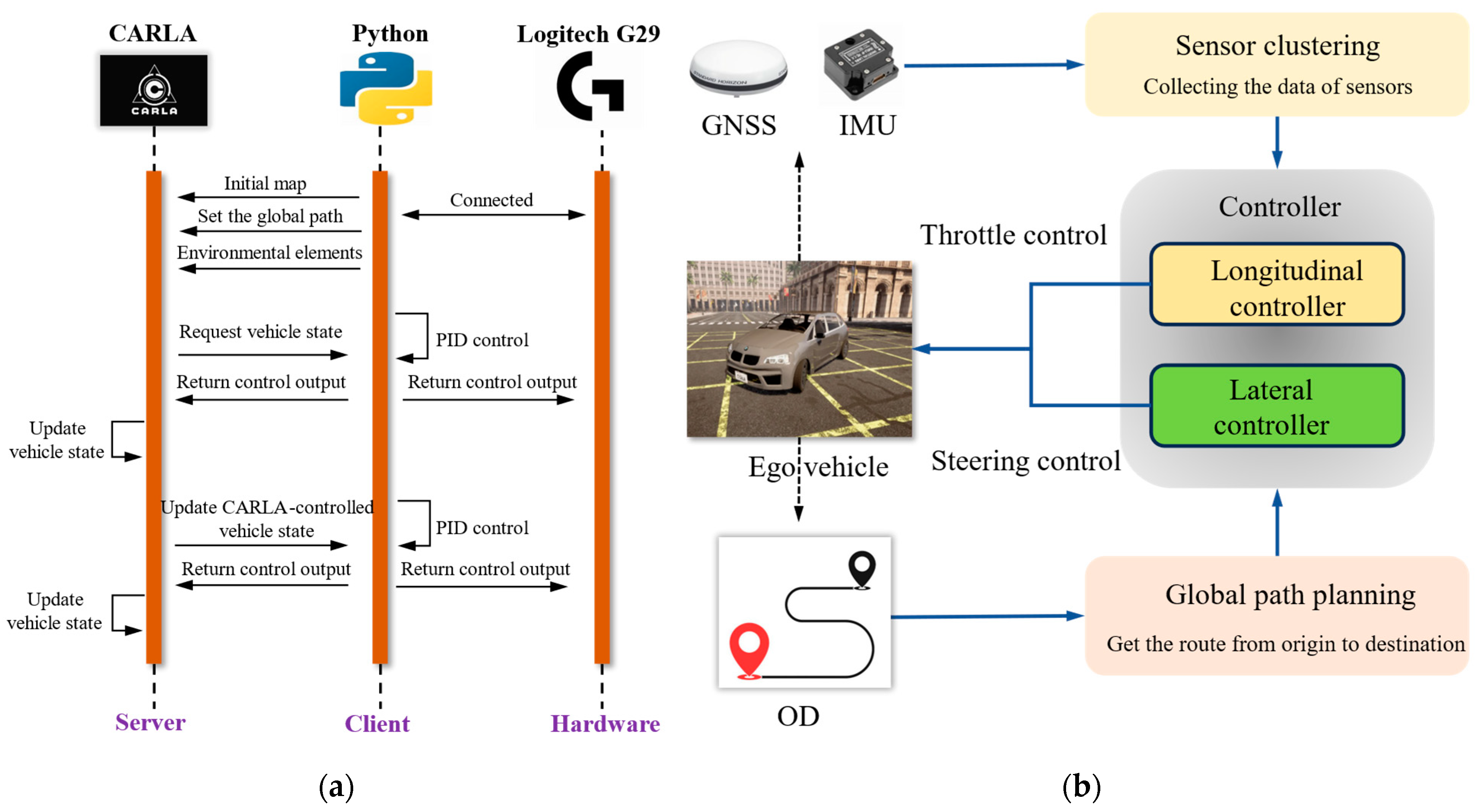
This study develops a comprehensive simulation environment for AV path tracking, considering various environmental perturbations. Specifically, this study employs CARLA [42], an open-source high-fidelity AV simulation platform that enables the design, testing, and validation of AV algorithms in realistic urban driving environments. The proposed simulation environment is shown in Figure 4a, which is designed to utilize a client/server (CS) architectural framework and incorporates external vehicular control hardware. In this simulation environment, CARLA, operating as the server, provides 3D static city scenes, realistic vehicle dynamic models, and various onboard sensors. The main interface for the client is Python scripts. By using a Python API, it is possible to select maps, change the weather, spawn various vehicles, and design vehicular control algorithms. Additionally, we have introduced Logitech G29’s virtual driving hardware [43] to observe specific vehicle operations visually.
In this paper, CARLA version 0.9.13 is utilized, and Figure 4b illustrates the AV path-tracking flow chart in our simulation environment. First of all, our simulation environment initializes the 3D urban map, spawns the autonomous vehicle, deploys onboard sensors, and defines the origin and destination (OD). Following these initial setup steps, the global path planning module leverages the A-star algorithm [44] to generate the global planning route that connects the specified origin and destination point. The A-star algorithm, also known as A*, is a popular pathfinding algorithm used in various applications such as AI for games, robotics, and autonomous driving systems. It is used to efficiently find the shortest path between two points in a graph- or grid-based environment, taking into account the obstacles and costs associated with different paths. In CARLA, the A-star algorithm can be employed to calculate optimal paths for autonomous vehicles to navigate from their current location to a desired destination. Within the control loop, the Global Navigation Satellite System (GNSS) is employed to accurately determine the vehicle’s position, and the Inertial Measurement Unit (IMU) supplies essential data regarding the vehicle’s speed and attitude. Simultaneously, by utilizing the vehicle’s state information, including position, speed, and heading angle, the PID controller generates control signals for the vehicle, i.e., the throttle and steering wheel angle commands, which dictate the desired actions to be executed. It is noted that the proposed environment encompasses a variety of perturbations, including city scenes, planning routes, weather conditions, road slopes, and various vehicle types. A further depiction of these perturbations is provided in Table 2.
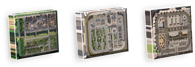
As illustrated in Table 2, various environmental perturbations are introduced to rigorously test the capabilities of the AV path-tracking system. Our study selected three distinct urban cities in the CARLA simulator. These urban locales encompass Town 1, a European-style town composed of solely one-line roads and T junctions. Moving on, Town 3 emerges as a more expansive urban landscape, mirroring the attributes commonly found in bustling downtown areas. Lastly, Town 10 hosts many junction arrangements with various lane markings, crossings, and signal types to challenge the autonomous vehicles in negotiating with other traffic. We curated 150 intricately designed routes in these three cities, encompassing various navigational complexities such as straight paths, turning maneuvers, and lane-changing scenarios. In addition to accounting for route diversity, our study also incorporates three distinct road types: flat terrain, uphill gradients, and downhill slopes. Recognizing weather’s impact on road surface adhesion coefficients and vehicle wind resistance, we have incorporated four distinct weather categories into our experimental framework: sunny, light rain, moderate rain, and heavy rain. Lastly, acknowledging that the vehicle type significantly influences its maneuvering capabilities, we provide a selection comprising an SUV, a compact sedan, and a mini-car for experimentation purposes. To the best of our knowledge, this paper is the first to synthesize multiple environmental perturbations for an in-depth examination of AV path tracking. The procedure of AV path tracking is shown in Algorithm 1.
Algorithm 1: PID control for AV path tracking.
Input :   k p , l o n g , k i , l o n g , k p , l o n g , k p , l a t , k i , l a t , k p , l a t #parameters of longitudinal and lateral PID controller
D r , D t , D e , I m a x , N # configuration for PID control algorithm
Output :   the   global   planning   route   G ,   the   historical   track   point   set   T ,   and   the   historical   lateral   acceleration   set     A l a t
1.  Initialize   the   environment ,   select   the   town ,   vehicle   type ,   OD   pair ,   and   weather ,   and   set   T =   ,     A l a t = { }
2.  Utilize   A - star   algorithm   to   generate   global   planning   route   G = x r , 1 , y r , 1 , x r , 2 , y r , 2 x r , n , y r , N ,   where   each   point   is   a   reference   point ,   and   the   distance   of   adjacent   reference   points   is   set   as   D r
3.  Set   F l a g   = 1 ,   i   = 1 ,   n   = 1.
4.  While   F l a g   == 1 do
5 . obtain   the   vehicle   position   x c , n , y c , n     using   GNSS ,   then   T T x c , n , y c , n
6.    obtain the vehicle velocity, acceleration, and heading angle using IMU
7 . obtain   the   lateral   acceleration   a c c l , n ,   then     A l a t   A l a t a c c l , n
8 . calculate   the   longitudinal - tracking - error -   and   lateral - tracking - error - based   current   reference   point   x r , n , y r , n
9 . calculate   the   throttle   ξ a c c   and   ξ s t e e r steering angle using Equations (8) and (9)
10.   execute the controller output and update the simulation
11 . calculate   the   distance   between   x c , n , y c , n   and   x r , n , y r , n ,   denoted   as   d i
12 . If   d i D t  then
13.     n = n + 1 # track the next reference point
14.    End if
15 . If   n = = N   and   d i D e  then
16.    Flag = 0
17.    End if
18 . If   i > I m a x  then
19.    Flag = 0
20.    End if
21 . i = i + 1
22. End while
In Algorithm 1, the PID control algorithm is implemented on the CARLA simulation platform for autonomous vehicle trajectory tracking. The process involved three main steps: environment initialization, global path planning, and PID control. Initially, the CARLA environment is set up, encompassing the selection of towns, weather conditions, and vehicle types. Subsequently, we define the origin and destination (OD) for the self-driving trip and utilize the A-star algorithm to generate a global planning route G = x r , 1 , y r , 1 , x r , 2 , y r , 2 x r , n , y r , N , wherein the distance between successive waypoints in G is denoted as D r . In this study, we set D r to 2 m. Finally, we employ longitudinal and lateral PID controllers to track the global path G . The parameters of the two controllers are denoted as k p , l o n g , k i , l o n g , k d , l o n g for the longitudinal controller, and k p , l a t , k i , l a t , k d , l a t for the lateral controller. Trajectory tracking is achieved by sequentially traversing the reference points in G . If the vehicle’s distance from the target point (denoted as d i ) is below the predefined threshold D t (set to 1.5 m in this study), the vehicle’s target point is updated to the subsequent point in G . This iterative process continues until either the distance between the vehicle and the destination becomes less than D e (set to 0.2 m in this study) or the number of iterations exceeds the maximum value I m a x . At that point, the PID control is terminated. The outputs of Algorithm 1 consist of the global planned route, the vehicle’s historical track point set, and the vehicle’s historical lateral acceleration set. In the subsequent section, we will utilize these results to evaluate the accuracy and smoothness for AV trajectory tracking.

2.4. PID Parameter Optimization Model

This paper attempts to achieve a trade-off between tracking accuracy and smoothness in AV path tracking. To this end, two corresponding evaluation indicators are introduced below.

2.4.1. Normalized Dynamic Time Warping

In AV path tracking, the tracking accuracy can be measured by the similarity between the globally planned path and the actual driving trajectory controlled by a PID algorithm. Trajectory similarity measures have garnered significant attention in various domains, leading to the development of numerous measurement techniques in the literature [45,46]. One of the most straightforward methods to measure the similarity between two trajectories is by calculating the spatial distance between corresponding points, such as the initial two points of each trajectory, the subsequent two points, and so forth. Subsequently, more sophisticated measures attempt to compare trajectories in more intricate ways. Dynamic time warping (DTW) stands as a classical dynamic programming algorithm that has been successfully utilized for measuring the similarity between trajectories [47,48]. In this paper, DTW is computed by aligning elements of a reference trajectory (i.e., the globally planned path G ) and a query trajectory (i.e., the actual driving trajectory T ) while preserving their order. Specifically, DTW finds the optimal ordered alignment between the two trajectories by minimizing the cumulative cost:
D T W G , T = min W W i k , j k W δ g i k , t j k
where δ is some distance function mapping pairs of elements from the two trajectories to real non-negative numbers and W = w 1,2 W is a warping with w k = i k , j k 1 : G × 1 : T , respecting the step-size ( w k + 1 w k 1,1 , 1,0 , 0,1 ), boundaries ( w 1 = 1,1 , and w W = G , T ) conditions. In AV path tracking, the cost function is the Euclidean distance between the coordinates of any two points in space. The ideal metric for evaluating the tracking error must be sensitive to the scale and density of the nodes along the actual driving trajectory. In order to address this, we propose a normalized DTW metric, which is defined as the sum of at least G distance terms, by normalizing it by a factor of 1 G . This normalization process allows for a fair comparison and consistent evaluation across different scenarios. Directly derived from DTW, the NDTW metric is shown in Equation (11).
N r = D T W G , T G = min W W i k , j k W δ g i k , t j k G
The principle of NDTW can be expressed in Figure 5, where the black lines in Figure 5a,b represent the point where the two tracks match and align. NDTW has many desirable properties for evaluating actual driving trajectories. It measures the similarity between the entirety of two trajectories, softly penalizing deviations.

2.4.2. Mean Absolute Lateral Acceleration

Mean absolute lateral acceleration (MALA) [49,50] is often used as a performance indicator to evaluate the smoothness of a vehicle’s motion. Lateral acceleration refers to the acceleration experienced by an occupant or passenger in a sideways direction perpendicular to the vehicle’s forward motion. It measures how much the vehicle deviates from a straight-line path during maneuvers such as turns or lane changes. A lower MALA indicates smoother vehicle motion, reducing the likelihood of passenger motion sickness and enhancing ride comfort. Hence, this paper adopts MALA as an evaluation metric for tracking smoothness. The MALA metric is represented by Equation (12).
M r = a c c   A l a t a c c   A l a t
where   A l a t represents the historical lateral acceleration set, which comprises multiple values of lateral acceleration (i.e., a c c ).   A l a t is the magnitude of the   A l a t , and a c c signifies the absolute value of a c c . Given the parameters of the lateral and longitudinal PID controller x = k p , l a t , k i , l a t , k d , l a t , k p , l o n g , k i , l o n g , k d , l o n g T , multiple independent simulation evaluations will yield varying N r and M r values owing to the perturbations in the simulation environment (e.g., randomly selected towns, routes, and weather conditions, etc.). Accordingly, the two objectives are represented as expectations relative to N r and M r , and the PID parameter optimization model is formulated as
min x X P x = E N r x , ζ , E M r x , ζ
s .   t .   Θ x , ζ N r x , ζ , M r x , ζ
In Equation (13), the feasible solution set is defined by X = x : l 1 x u 1 . The exogenous parameters ζ encompass both fixed (e.g., vehicle dynamic model and tire model) and stochastic (e.g., uncertainties in towns, routes, weather, and vehicle types) factors within the simulation environment. The simulation platform, denoted by Θ x , ζ , processes inputs x and ζ with the mapping operator , yielding the simulation outcomes. N r x , ζ and M r x , ζ denote the resultant values for N r and M r , obtained from the simulation given the inputs x and ζ . The expectation E · considers the stochastic parameters in ζ and is calculated with respect to N r or M r . It is evident that model (13) seeks to simultaneously minimize the expectations related to N r or M r . In the next section, the DMEGO algorithm will be utilized to solve this model.

3. Methodology

We first provide a detailed introduction to the EGO algorithm. Readers already acquainted with the Gaussian process and expected improvement may proceed directly to Section 3.2. In Section 3.2, we propose a domination-measure-based efficient global optimization algorithm (DMEGO) for a multi-objective simulation optimization problem.

3.1. Efficient Global Optimization

As a prelude, a powerful framework namely EGO was proposed for single-objective global optimization problems with implicit functions that are expensive to evaluate. With the help of a surrogate model and acquisition function, the framework consists of three pivotal steps: (1) Utilizing a cost-effective surrogate model to estimate the implicit function based on solutions evaluated using true objective functions or simulations; (2) Designing an acquisition function that guides the optimization process toward promising solutions with improved performance and reduced uncertainty; (3) Selecting a candidate solution via the optimization of the acquisition function, evaluating it by the true objective function, and updating the surrogate model.

3.1.1. Gaussian Process

A Gaussian process (GP) [51] is a statistical approach to model probability distributions over functions. It is concisely defined by a prior mean function denoted as m · and a covariance function represented as k · , · . As a widely favored surrogate model, the GP provides an estimation of the real objective function using a set of previously evaluated solutions. Let x 1 : n = x 1 , , x n T be a finite collection of evaluated solutions, where x i R D , i = 1 , , n , and their corresponding objective function values are f 1 : n , where f i = f x i . Thus, the GP prior is expressed with a multivariate normal distribution:
f 1 : n ~ N m 1 : n , K x 1 : n , x 1 : n
Consider m 1 : n to be the vector containing the mean function values, with each m i corresponding to m x i . Let K x 1 : n , x 1 : n be the covariance matrix, and the element at position i , j is denoted by k x i , x j , quantifying the covariance between x i and x j . When dealing with situations where the objective function’s form is entirely unknown, a typical approach involves utilizing a zero or constant as the prior mean. For the covariance function, the power exponential kernel is often preferred, defined by the following expression:
k x i , x j = σ 0 2 e x p x i x j 2 2 2 l 2
In Equation (15), x i x j 2 represents the Euclidean distance between x i and x j , while σ 0 2 and l are parameters of the power exponential kernel. The analytical tractability of the GP is one of the factors that contributes to its popularity. As indicated in Equation (14), the true objective function values (i.e., f 1 : n ) follow a joint Gaussian distribution based on the GP prior. Similarly, for a new sample x s , the estimate of the objective function f x s is also expected to follow a jointly Gaussian distribution with the GP prior, which can be mathematically expressed as follows:
f 1 : n f x s ~ N m 1 : n m x s , K x 1 : n , x 1 : n k x 1 : n , x s k x s , x 1 : n k x s , x s
where   k x s , x 1 : n = k x s , x 1 , , k x s , x n
k x 1 : n , x s = k x s , x 1 : n T
We can consider the solutions x 1 : n and their true objective function values f 1 : n as historical observations, while x s and f x s represent a newly sampled solution and its estimate for an objective function, respectively. By conditioning on them, we can restrict the distribution of possible functions predicted by the GP, which is referred to as the GP posterior. When there are noisy observations (e.g., Gaussian noise with variance τ 2 ), the predicted distribution-based n observations follow a Gaussian distribution characterized by a posterior mean value μ n x s and a posterior variance value σ n 2 x s :
f x s | f 1 : n ,   x 1 , , x n ~ N μ n x s , σ n 2 x s
μ n x s = m x s + k x s , x 1 : n K x 1 : n , x 1 : n + τ 2 I 1 f 1 : n m x s
σ n 2 x s = k x s , x s k x s , x 1 : n K x 1 : n , x 1 : n + τ 2 I 1   k x 1 : n , x s
where I is the identity matrix. The inverse operation on the matrix K x 1 : n , x 1 : n + τ 2 I demands computational effort scaling with O ( t 3 ) , which can become computationally intensive when the observation count is substantial (for instance, upwards of 10 5 observations). Nevertheless, it is essential to highlight that in the context of SO, the number of observations typically remains comparatively limited, thereby mitigating concerns related to computational scalability.

3.1.2. Acquisition Function

The acquisition function utilizes the posterior mean and variance derived from the GP to determine the next solution for evaluation. From a minimization perspective, choosing a solution with a low posterior mean function value indicates exploitation, whereas opting for a solution with a high posterior variance signifies exploration. As such, the acquisition function encompasses both μ n · and σ n 2 · . To determine the next solution for evaluation, it is necessary to maximize the acquisition function.
Research on the BO algorithm has introduced several acquisition functions formulated using analytical expressions, including but not limited to the probability of improvement [52], expected improvement [53], and the upper confidence bound [54]. In this paper, we employ the expected improvement (EI) acquisition function for the minimization problem, which is defined as follows:
E I x = E m a x 0 , f m i n f x
= f m i n μ n x Φ Z + σ x ϕ Z
Where   Z = f m i n μ n x σ x
where f m i n represents the smallest estimated objective function value among all evaluated solutions. The function Φ · and ϕ · in Equation (23) represent the probability density function and cumulative distribution function of the standard normal distribution, respectively. The process of selecting the next evaluation point (denoted as x ) can be achieved by solving the subsequent maximization problem:
x = arg max x X E I x
Figure 6 illustrates a 1D optimization problem solved using the GP posterior and acquisition function. The green dots represent the observed data points used for fitting the GP, resulting in the posterior mean function represented by the red solid line and the posterior variance depicted by the shaded region. The true objective function is illustrated by the black solid line, while the EI acquisition function is represented by the blue solid line. From the figure, it can be observed that the EI acquisition function attains its peak values in regions where a low posterior mean function value coincides with a large posterior variance. Using iterative steps involving the construction of the GP model, the calculation for the EI function, and the selection of the next solution, the EGO algorithm gradually converges to a globally optimal solution.

3.2. Domination-Measure-Based Efficient Global Optimization

There exist several approaches to expand the scope of the EGO algorithm for addressing multi-objective simulation-based optimization problems. The most straightforward approach, referred to as ParEGO, entails transforming multi-objective values into a single objective value by employing a parameterized scalarizing weight vector. By selecting a different weight vector at each search iteration, it becomes feasible to progressively generate an approximation of the entire true Pareto front. The BOEGO algorithm extends the EGO to address multi-objective scenarios by integrating two regressive kriging models and employing an EI infill strategy. Nevertheless, based on our current knowledge, none of the prior methods consider diversity in the performance space, which can be critical for numerous multi-objective problems encountered in real-world scenarios.
Without losing generality, we assume a SO problem that seeks to minimize M objective functions. Firstly, we use M GP models to approximate M true objective functions, respectively. Then, the key insight of our acquisition function is that instead of finding an M -dimensional Pareto front corresponding to M objectives, it finds a 2 M -dimensional Pareto front where M dimensions correspond to the performance objectives (each given by μ n m x , m = 1 , , M ) and other M dimensions correspond to the uncertainty of those objectives ( σ n m x , m = 1 , , M ). In other words, our acquisition function A f · simultaneously minimizes the predictive mean functions and maximizes the posterior variance based on M GP models:
x = arg min x X A f x = μ n m x , σ n m x , m 1 , M
In Equation (26), finding a solution within the feasible region X that simultaneously minimizes all the objectives is extremely rare. Therefore, a compromised target is to identify all non-dominated solutions in X based on their objective values. More specifically, the domination rule, Pareto optimal solutions, and Pareto front for problem (26) are defined as follows:
Definition 1.
Let  x u ,   x v X  be two solutions. We state that  x u  dominates  x v  (denoted by  x u x v if and only if  μ n m ( x u ) μ n m ( x v )  and  σ n m ( x u ) σ n m ( x v ) ,  m { 1 ,   2 , , M } and  l { 1 ,   2 , , M }  such that  μ n l ( x u ) < μ n l ( x v )  or  μ n l ( x u ) > μ n l ( x v ) .
Definition 2.
A solution  x X  is considered to be a Pareto optimal solution if and only if    x X \ { x }  such that  x x The set of Pareto optimal solutions is known as the Pareto optimal set, and its representation in the objective space is referred to as the Pareto front.
Inspired by [55], this study introduces a unary and parameter-free performance metric called domination measure, to measure the quality of a solution under multiple evaluation criteria with no distinction between objectives. Specifically, this measure can be understood as the likelihood that a randomly chosen solution from the feasible region X dominates that solution according to a predefined probability measure. So, x X , the domination measure for x is defined as follows:
D x = v D x v X = X 1 y x v d y X v d y = X 1 y x U d y E U ( y ) 1 y x
where D x represents the collection of solutions that dominate x , while v ( · ) corresponds to the underlying Lebesgue measure, and U · denotes the probability distribution on X induced by v ( · ) . The indicator function 1 E equals 1 when event E is true and 0 otherwise. E U [ · ] represents the expectation with respect to U · . Several properties of the domination measure in X can be straightforwardly established: (1) For any x X , it holds that 0 D x 1 ; (2) If y x , then D y D x ; (3) For any Pareto optimal solution x P * , where P * is the Pareto optimal solution set in X , then D x = 0 . We present a numerical example demonstrating the advantages of using the domination measure to evaluate the solution quality in a multi-objective scenario.
Example 1.
Consider a bi-objective optimization problem [56] with a nonconvex Pareto optimal set:
min f 1 x = 0.001 x x 10 x 60 x 100 + 1000 min f 2 x = 0.001 x x 70 x 100 x 200 + 6000 s . t .   x ϵ z 0 , 100
With no further elaboration here, the Pareto optimal set for Example 1 is  z ( 5,25 60,85 ) , and it is highlighted with green and purple bold lines in Figure 7.
Directly utilizing the two objective functions to locate the Pareto optimal set for Example 1 is difficult and unintuitive, so we take two methods to rigorously quantify the quality of a solution, respectively, i.e., the domination measure and the linear weighted sum method. Firstly, the domination measure D ( x ) and the linear combination of the bi-objectives (i.e., w 1 f 1 x + w 2 f 2 x ) are calculated for each solution in the finite solution space, and the quality of a solution is easily obtained from Figure 8. Note that the latter method is parameter-based: without a loss of generality, we set five groups of weighting coefficients to represent the different preference degrees for the bi-objective functions.
As shown in Figure 8, although both methods can strictly evaluate the solution quality using a deterministic scalar, the domination measure exhibits significant advantages in the following two aspects: (1) We can readily and directly identify the Pareto optimal set in Figure 8a by considering the fundamental principle that a smaller domination measure indicates a superior solution quality. In other words, solutions with a domination measure of zero precisely constitute the Pareto optimal set for Example 1. In Figure 8b, even a solution x 1 dominates another solution x 2 ; the linear weighted sum of x 1 is not always lower than that of x 2 . This inconsistency arises from the potential loss of information regarding the dominance relationship due to applying a weighting scheme to the bi-objective functions. Thus, the linear weighted sum method cannot effectively characterize the dominance relationship between solutions, which results in relatively good solutions rather than the Pareto optimal set. (2) As a parameter-free performance metric, the domination measure does not depend on any fixed parameters. However, the linear weighted sum method requires first customizing the weighting coefficients, which would considerably impact evaluating the quality of a solution. Specifically, the larger the w 1 in Figure 8b, the more the linear weighted sum method prefers the solutions in z 60,85 and vice versa for solutions in z 5,25 . Consequently, the quality evaluation of solutions using the linear weighted sum method varies considerably under different weighting coefficients, making the selection of suitable coefficients challenging. In contrast to the linear weighted sum method, the domination measure does not necessitate parameter tuning and offers a rigorous and precise quantification of solution quality in multi-objective problems.
In this paper, we focus on a sequential selection strategy, which suggests a single optimal sample for evaluation in each iteration. However, the maximization problem for the acquisition function (26) aims to find a set of solutions rather than a single solution. Therefore, we propose a domination-measure-based efficient global optimization algorithm to solve multi-objective SO problems in a sequential selection manner. Specifically, the DMEGO algorithm iteratively carries out the following four main steps: (1) independently construct M separate GP models for each objective function using evaluated observations; (2) employ the widely used NSGA-II algorithm to solve the maximization problem for the acquisition function, and obtain a set of promising candidate solutions; (3) utilize the domination measure and the crowding distance to selectively retain a candidate solution exhibiting superior performance and good diversity for the next iteration; (4) evaluate the ultimately selected candidate solution using true objective functions. In summary, the procedure of the DMEGO algorithm is shown in Algorithm 2.
Algorithm 2: Detailed computational process of the proposed DMEGO method.
Input :   the   dimension   of   decision   variable   D ,   the   num   of   objective   functions   M ,   the   true   evaluation   function   F · ,   the   num   of   initial   observations   s ,   maximum   number   of   iterations   N m a x ,   the   population   size   N p ,   and   generations   N g of NSGA-II.
Output :   a   Pareto   optimal   solution   set   H p .
1.: Initialization:
2 . :   Generate   s   initial   solutions   x 1 , x 2 , , x t , , x s ,   and   evaluate   them   using   an   expensive   evaluation   function ,   i . e . ,   evaluate   F x 1 , F x 2 , , F x t , , F x s   for   M   objectives .   Let   the   set   of   evaluated   solutions   H s = x 1 , x 2 , , x t , , x s ;   the   set   of   evaluated   multi - objective   function   values   F s = F x 1 , F x 2 , , F x t , , F x s ,   where   F x t = f 1 x t , f 2 x t , , f m x t , , f M x t T .
3 . :   Generate   Pareto   optimal   solution   set   H p   by   utilizing   the   fast   nondominated   sorting   method   with   H s .   The   set   of   evaluated   multi - objective   function   values   corresponding   to   H p   is   F p .   σ 0   and   σ m i n   represent   the   initial   value   and   threshold   value   of   the   percent   quantile   σ ,   and   τ   is   the   decay   factor   of   σ .   Set   n = 1 .
4 .   While   n N m a x do
5 . n = n + 1 ,   σ = m i n σ 0 × τ , σ m i n .
6 . Train   M   independent   GP   models   G m · , m = 1,2 , , M   on   H s   and   F s for each true objective function
     f m · , m 1,2 , , M .
7 . Utilize   the   NSGA - II   algorithm   to   solve   the   problem   max x X A f x = μ n m x , σ n m x , m 1 , M ,   where   μ n m x   and   σ n m x , m 1 , M   can   be   calculated   using   Equations   ( 20 )   and   ( 21 )   based   on   M   independent   GP   models .   Then ,   generate   the   set   of   candidate   Pareto   optimal   solutions   H c = x c 1 , x c 2 , , x c N p   and   the   set   of   predicted   multi - objective   function   values   F c = g x c 1 , g x c 2 , , g x c i , , g x c N p ,   where   g x c i = μ n 1 x c i , μ n 2 x c i , , μ n M x c i T .
8 . H n H s H c ,   F n F s F c .   For   i = 1 , ,   N p ,   estimate   the   domination   measure   D x c i = 1 H n y H n 1 y x c i ,   where   the   domination   rule   is determined by F n .   Sort   the   estimates   D x c i   in   ascending   order ,   denoted   by   D x c 1 D x c 2 D x c N p .   Set   the   reference   value   γ n   to   be   the   sample   σ - percent   quantile   D x c σ N p ,   that   is ,   γ n = D x c σ N p ,   where   σ N p   is   the   smallest   integer   that   is   greater   than   or   equal   to   σ N p .
9 . Reconstruct   the   set   of   candidate   Pareto   optimal   solutions   by   H c = x | D x γ n , x H c .   Then ,   find   a   solution   x   in   H c   that   has   the   largest   crowding   distance   for   F p .
10 .     Call   the   expensive   evaluation   function   F ·   with   the   solution   x .   Then ,   H s H s x ,   F s F s F x .
11 .       By   utilizing   the   fast   nondominated   sorting   method   with   H s ,   the   Pareto   optimal   solution   set   H p   and   its   corresponding   multi - objective   function   values   F p can be obtained.
12. End while
The DMEGO algorithm is proposed to address the multi-objective simulation-based optimization problem. Algorithm 2 provides a general overview of the entire flow of DMEGO. However, when applying the DMEGO algorithm to solve the PID parameter optimization problem (referred to as problem (13)), it becomes necessary to clarify specific details. Initially, the decision variable dimension, D , is set to 6, indicating three parameters each for the longitudinal and lateral controllers. Subsequently, there are only two objective functions: NDTW and MALA. Lastly, the true evaluation function F · is composed of Algorithm 1 and Equations (11) and (12), representing the complex mapping relationship between the NTWR, MLSA, and PID control parameters. In Section 4.2, the DMEGO algorithm will be employed to solve the PID control parameter optimization problem.

4. Numerical Experiments

This section begins by conducting a comprehensive evaluation of the proposed DMEGO algorithm. Subsequently, the DMEGO algorithm is applied to tackle the PID controller parameter optimization problem. To test the effectiveness of the DMEGO algorithm and perform a comparative analysis with other competing algorithms, we employ the inverted generational distance (IGD) metric [57] and the diversity metric ( Υ ) [58] to quantify the convergence and diversity of DMEGO. More specifically, the IGD metric, defined in the objective space, is expressed as:
I G D = 1 R y R min x Z F x F y 2
Let R be a designated reference set containing R evenly distributed points from the true Pareto front (TPF). The function vector F · = f 1 · , f 2 · , , f M · comprises the collection of true objective functions. Meanwhile, Z denotes the approximate Pareto front (APF) produced by the evaluated algorithm. The IGD metric quantifies the average proximity between the members of the reference set and the approximate Pareto front, essentially measuring how well the APF mirrors the TPF. Thus, a lower IGD metric indicates superior convergence and diversity.
Before discussing the diversity metric Υ in the solution space, it is essential to sequence the Z approximate Pareto optimal solutions x 1 , x 2 , , x Z produced by the evaluated algorithm, in ascending order based on the f 1 · criterion, such that f 1 x 1 f 1 x 2 f 1 x Z . Furthermore, x 1 and x Z denote the extremities of the APF, termed the leftmost and rightmost boundary points, correspondingly. Similarly, x l and x r represent the extremities of the TPF. The diversity metric Υ is then described below:
Υ = d l + d r + i = 1 Z 1 d i d ¯ d l + d r + Z 1 d ¯
where d l = x l x 1 ( d r = x r x Z ) is the distance between the leftmost (rightmost) boundary point of the APF and the leftmost (rightmost) boundary point of the TPF. d i = x i + 1 x i refers to the distance between an approximate Pareto solution and its closest neighbor, whereas d ¯ = 1 / Z 1 × i = 1 Z 1 d i denotes the average of these distances. In essence, Υ quantifies the evenness of the distribution of solutions in the solution space. Clearly, a smaller Υ value shows better diversity.

4.1. A Benchmark Test Problem

This study employs a challenging benchmark test problem (30), essentially a stochastic adaptation of the FON function proposed by [59]. The test problem (30) introduces stochastic perturbations into each objective function, thereby complicating the relationship between potential solutions and the expected outcomes of the bi-objective functions. Moreover, these stochastic variations also make the dominance relationships between any pair of solutions less apparent. In light of these challenges, we compare the performance of DMEGO against three other state-of-the-art algorithms, namely NSGA-II [60], ParEGO, and BOEGO, in addressing the problem (30). To facilitate a fair comparison among these four algorithms, we set a fixed budget of 200 function evaluations for this numerical case.
min x f x = E f 1 x , ζ , E f 2 x , ζ
where   f 1 x , ζ = 1 e i = 1 3 x i 1 3 2 + ζ
f 2 x , ζ = 1 e i = 1 3 x i + 1 3 2 + ζ
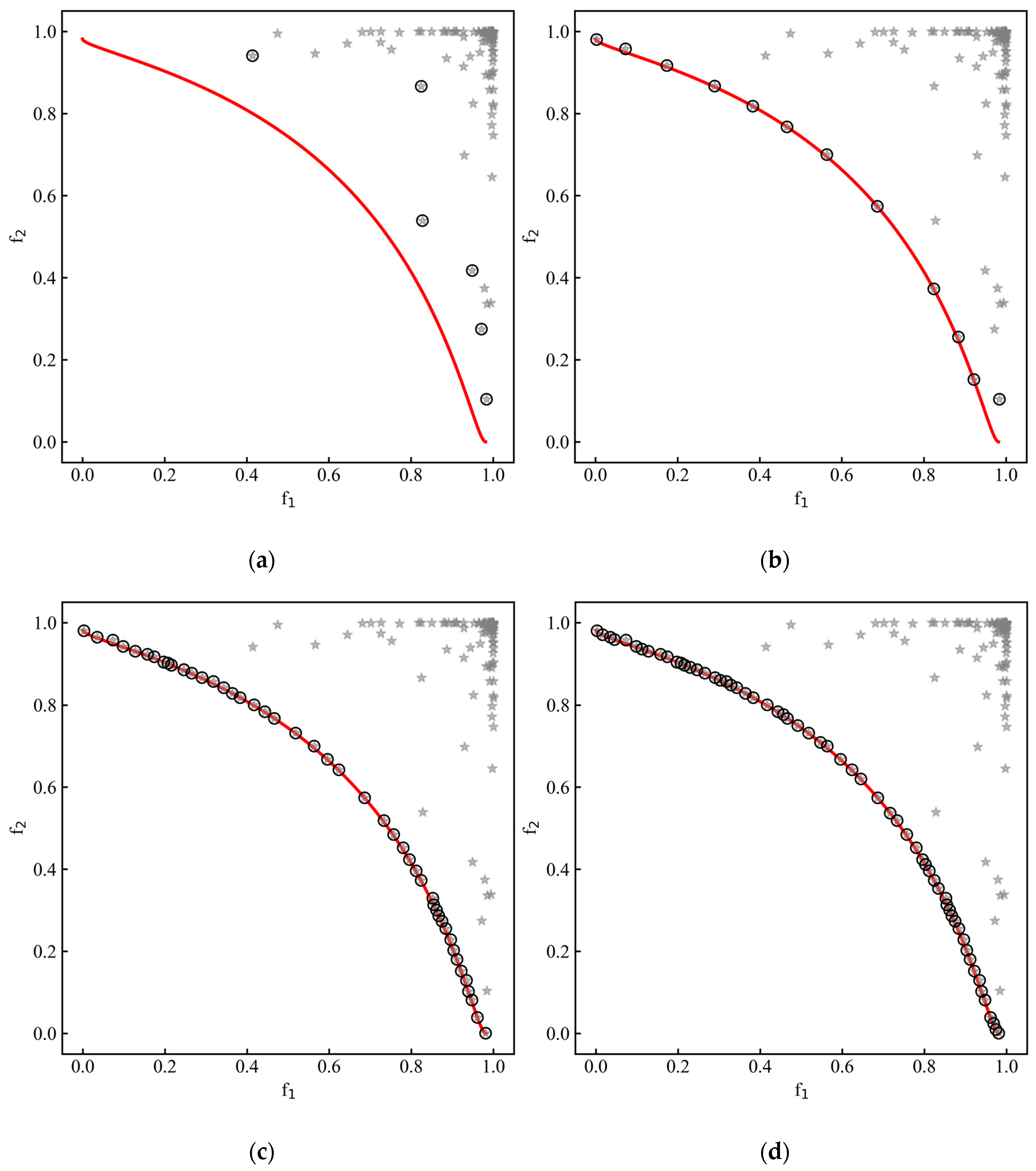
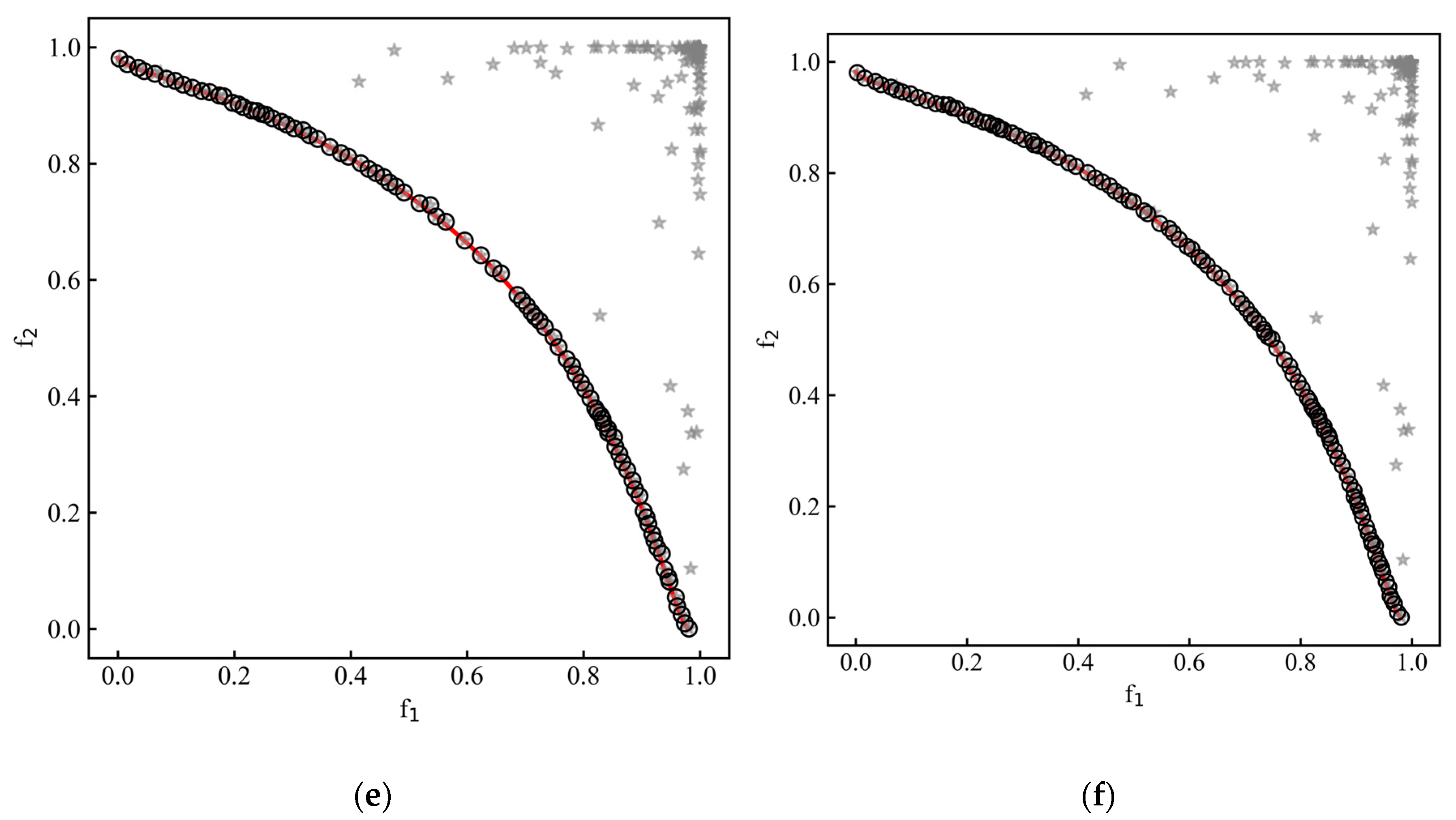
In problem (30), x = x 1 , x 2 , x 3 T and x i 2,2 , i = 1, 2, 3. The white noise is ζ ~ N 0 , 0.1 . Its true Pareto optimal solutions are x 1 = x 2 = x 3 1 3 , 1 3 . To offer further insights into the convergence of the DMEGO algorithm toward the true Pareto front, we present an illustrative depiction in Figure 9. Each subgraph in Figure 9 corresponds to an iteration of the algorithm. The red solid line represents the TPF of the problem (30), the gray pentagrams represent the evaluated solutions selected by DMEGO up to this iteration, and the black circles denote the nondominated solutions among the evaluated solutions. It is evident that DMEGO method is capable of obtaining evenly spread Pareto optimal points and capturing the entire Pareto front for the problem (30) using a remarkably limited number of function evaluations.
Obviously, Figure 10 demonstrates the superiority of the nondominated solutions obtained using the DMEGO algorithm in terms of diversity and closeness to the TPF compared to the results obtained by the other three algorithms. Specifically, the nondominated solutions obtained using NSGA-II exhibit a considerable distance from the TPF, indicating the limited applicability of NSGA-II in addressing the problem (30) under restricted computational resources. As for ParEGO, although most nondominated solutions lie on the TPF, they exhibit sparsity and insufficient spread. BOEGO generates more nondominated solutions lying on the TPF. However, there are still some solutions that deviate from the TPF. Our proposed DMEGO method yields more nondominated solutions than the other algorithms, and all solutions exhibit excellent spread and precise alignment with the TPF. More detailed comparison results are presented in Table 3, which reveal that, despite the limited computational costs, DMEGO achieves a perfect Pareto front with superior convergence and diversity (evidenced by a smaller IGD value and a smaller Υ value). In conclusion, due to limited evaluation resources, the other three algorithms inefficiently utilize a large portion of samples by focusing on expanding a single region and encountering difficulties in escaping local minima. In contrast, our proposed DMEGO algorithm efficiently explores and identifies all regions comprising the TPF.
Additionally, we visualize the iterative process in the DMEGO algorithm to validate its superiority and effectiveness. Figure 11a,b demonstrate that, after about 125 function evaluations, the IGD and HV using DMEGO remain relatively stable and notably outperform NSGA-II, ParEGO, and BOEGO. Finally, we employ K-fold cross-validation (KFCV) to evaluate the estimation errors of the two GP surrogate models for the bi-objectives during the iterations of DMEGO. The errors are quantified using two widely recognized indices, namely the mean absolute percent error (MAPE) and root mean square error (RMSE). Figure 11c illustrates that estimation errors are initially high with a small number of samples but gradually decrease as the sequential selection scheme generates more data points. After about 50 function evaluations, the RMSE and MAPE decrease to as low as approximately 0.09 and 5%, respectively. This demonstrates that the Gaussian process model consistently improves in accuracy and reliability throughout the iterative process, effectively guiding the DMEGO algorithm toward the appropriate exploration region.

4.2. PID Parameter Optimization Problem Using the DMEGO Method

In this section, we utilize the DMEGO method to solve the PID parameter optimization problem (13) for AV path tracking. The PID controller parameters x have six dimensions, with three dedicated to the longitudinal controller and the remaining three for the lateral controller. NDTW and MALA serve as two objective functions for evaluating the tracking error and smoothness, and their true function evaluations require expensive simulations to collect tracking results (refer to Algorithm 1). Our experiment is tested using Intel(R) Xeon(R) E5-2620 v4 CPUs and NVIDIA GeForce RTX 2080 GPUs, and each true function evaluation takes about 2 min. The critical parameters of DMEGO (refer to Algorithm 2) are set as s = 200, N m a x = 400, N p = 200, N g = 200, σ 0 = 0.8, σ m i n = 0.1, and τ = 0.99. A total of 600 simulations were conducted, with 200 dedicated to the initial sampling (i.e., s = 200) and 400 to the algorithm’s iterative process (i.e., N m a x = 400). In the DMEGO method, NSGA-II is utilized as a solver for the acquisition function. Here, N p and N g represents the population size and generations in NSGA-II, respectively. Moreover, σ 0 , σ m i n , and τ automatically balance exploitation and exploration.
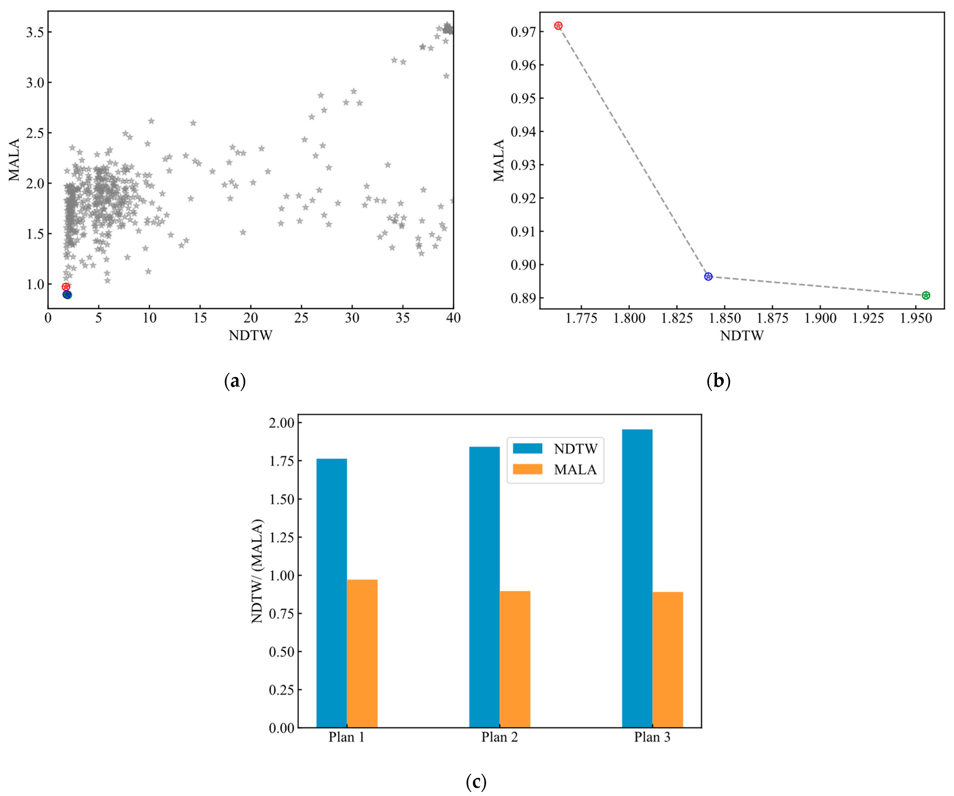
As illustrated in Figure 12, the DMEGO algorithm successfully obtains three Pareto nondominated solutions (represented by red, green, and blue circles) after conducting 600 costly simulation evaluations (indicated by gray pentagrams). Specifically, in Figure 12a, it is evident that the optimization process gradually improves the NDTW metric from an initial value of approximately 40 to within 2. Additionally, the MALA metric is optimized from its initial value of approximately 3.5 to within 1. Figure 12b,c present a comprehensive depiction of the three nondominant solutions, referred to as Plan 1, Plan 2, and Plan 3. Notably, an inverse relationship is evident: as the NDTW value ascends, the MALA value descends. This observation underscores the trade-off between the tracking accuracy and smoothness, highlighting their mutually exclusive nature in AV path tracking. More detailed results for these three nondominated solutions are presented in Table 4.
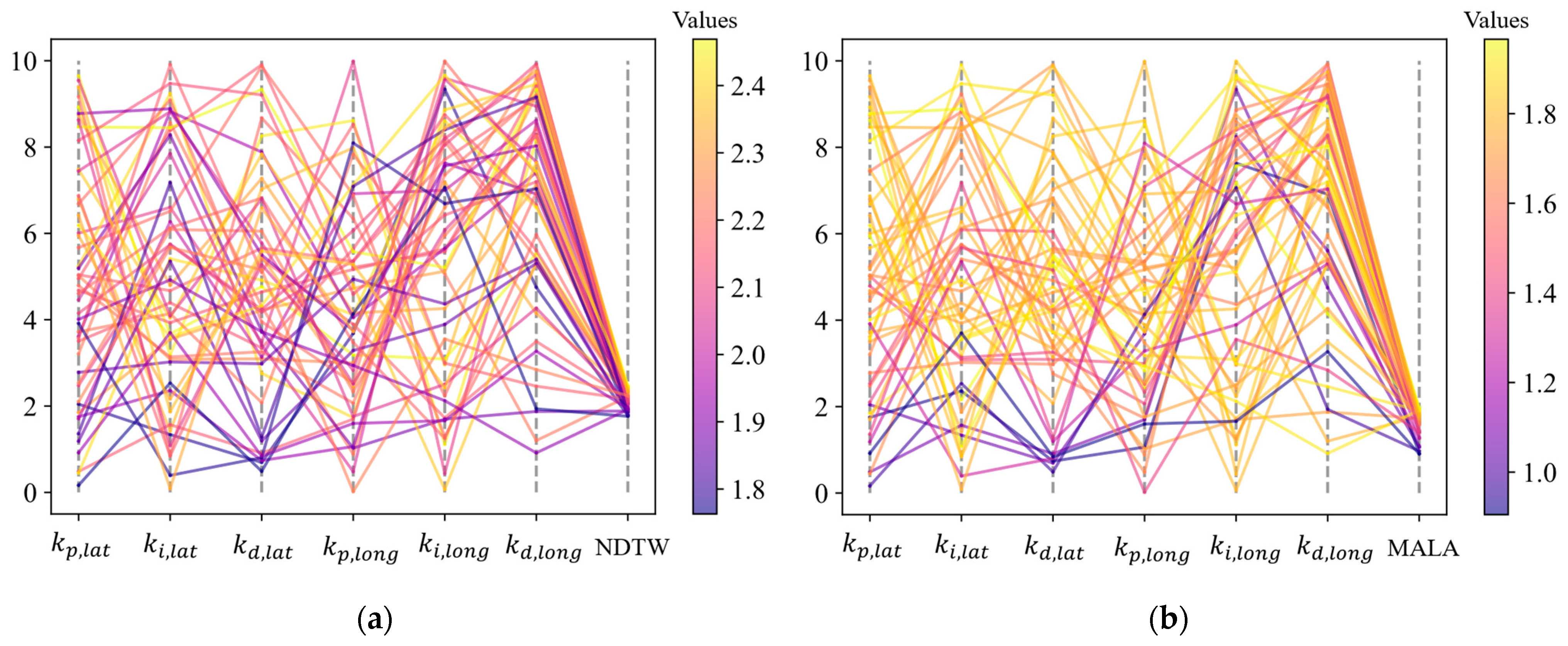
In addition to presenting the three optimized plans obtained by the DMEGO method, we also explore the influence of the PID parameters on the path-tracking performance of autonomous vehicles. After 600 simulation evaluations using the DMEGO algorithm, we select the last 50 solutions. Their distribution in the solution space is depicted in Figure 13. Each line in Figure 13 represents a set combination of six parameters of the lateral and longitudinal PID controller, and the line’s color reflects the tracking performance (the more purple the color, the better the performance). It can be seen from the figure that the vast majority of runs have bi-objective values below 2, which reflects the excellent stability of the DMEGO algorithm. Furthermore, as shown in Figure 13a, it is evident that higher values of k p , l o n g and k i , l o n g lead to a substantial improvement in tracking accuracy. This improvement can be attributed to the fact that increasing the k p , l o n g parameter enables the vehicle to achieve faster acceleration or deceleration, thus effectively tracking the desired speed. The k i , l o n g parameter is utilized to mitigate the accumulation of speed deviations and ensure the vehicle maintains a stable speed. Thus, increasing the k i , l o n g parameter could enhance the speed stability. Likewise, as depicted in Figure 13b, it is evident that reducing the values of k p , l a t and k d , l a t considerably enhances the tracking smoothness. Nevertheless, raising the k p , l a t parameter amplifies the control system’s sensitivity to lateral errors, enabling the vehicle to rectify deviations promptly. It is important to note that excessively high values of k p , l a t may result in overshooting and oscillation. Thus, the k p , l a t value should not be set too high. On the other hand, it is crucial to avoid excessively high k d , l a t values as they may introduce sensitivity into the noise, thereby diminishing the robustness of the PID controller.
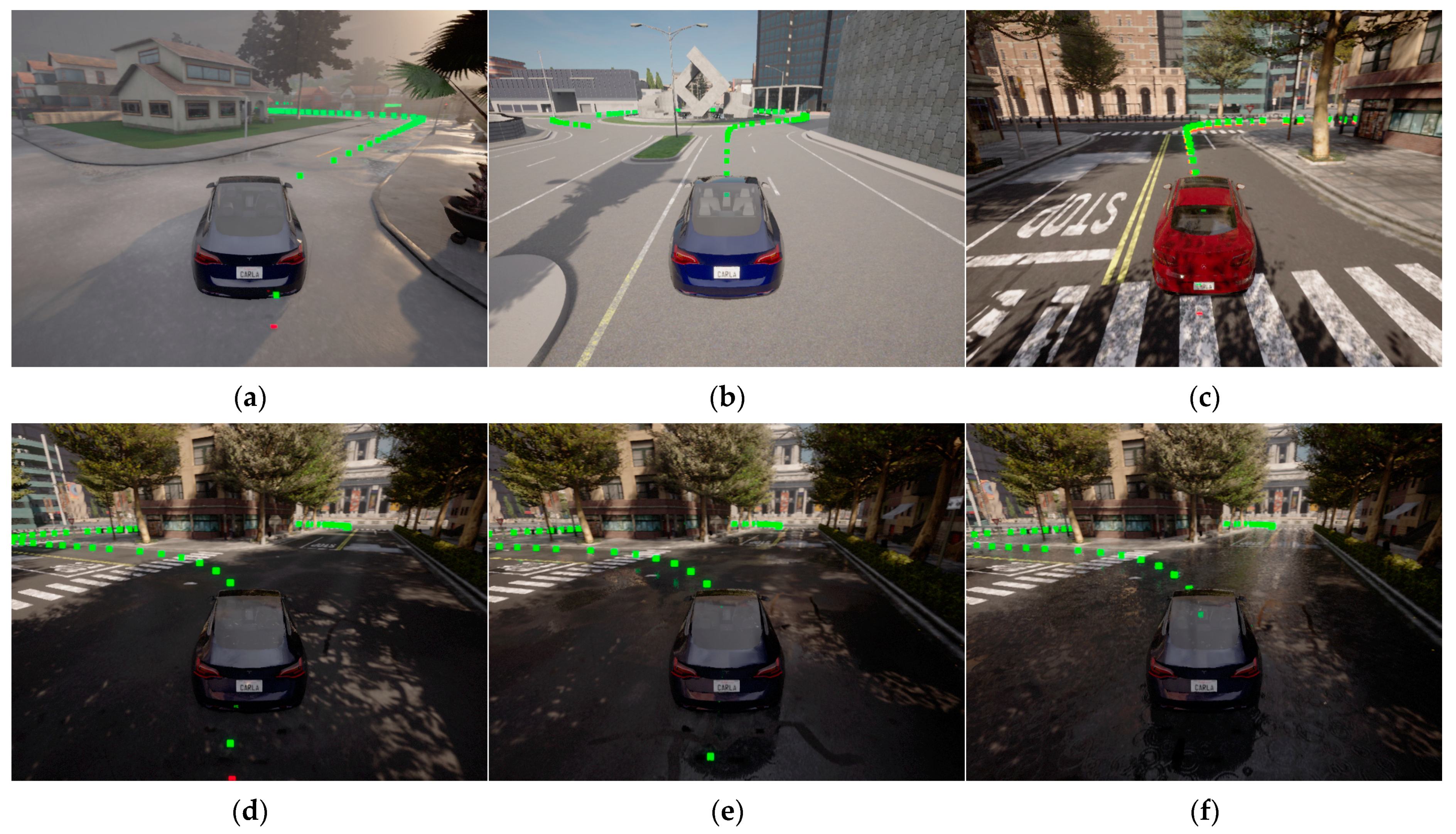
To strike a balance between the tracking accuracy and smoothness, we choose Plan 2 as the final scheme. Finally, we conduct comprehensive tests on the PID controller configured with Plan 2 in our proposed simulation environment, taking into account the presence of stochastic noise. This environment encompasses different city scenes, diverse routes, and various vehicle types, among other factors. Figure 14 presents a 3D visualization of our experimental scenarios. The green points depict the global route planned using the A-star algorithm for the autonomous vehicle, while the red points represent the target points that have been traversed. We select three towns, namely Town 1, Town 3, and Town 10, to create a diverse testing environment encompassing various urban environments and road characteristics. Specifically, Town 1 represents a relatively simple urban environment, making it suitable for initial testing and performance evaluation. Town 3 represents a moderately complex urban environment with straight and curved roads, varying road widths, and complex intersections, which may involve traffic lights, roundabouts, or multi-lane junctions. Town 10 represents a highly challenging and complex urban environment characterized by straight roads, sharp turns, complex junctions, and narrower streets. Furthermore, we have considered three distinct weather conditions: light rain, moderate rain, and heavy rain. The varying levels of ground wetness associated with these weather conditions result in variations in the adhesion coefficient of the road surface, posing a significant challenge to the path tracking of automated driving systems. In this paper, we have examined three different vehicle types in this study: van, car, and mini car. These vehicles exhibit varying body lengths and maneuvering stability levels, which can impact the performance of the PID controller. For a more intuitive demonstration of the experimental effects of Plan 2 discussed in this paper, a video version of the AV path tracking can be found in Supplementary Materials Video S1. As we can see from the video, our optimized PID control parameters can be adapted to various challenging scenarios, such as sharp turns, narrow roads, and even roundabouts. Notably, the controller performs well even in heavy rain and can be applied to a wide range of vehicles, highlighting the robustness of our optimized PID parameters against environmental perturbations in real-world conditions.
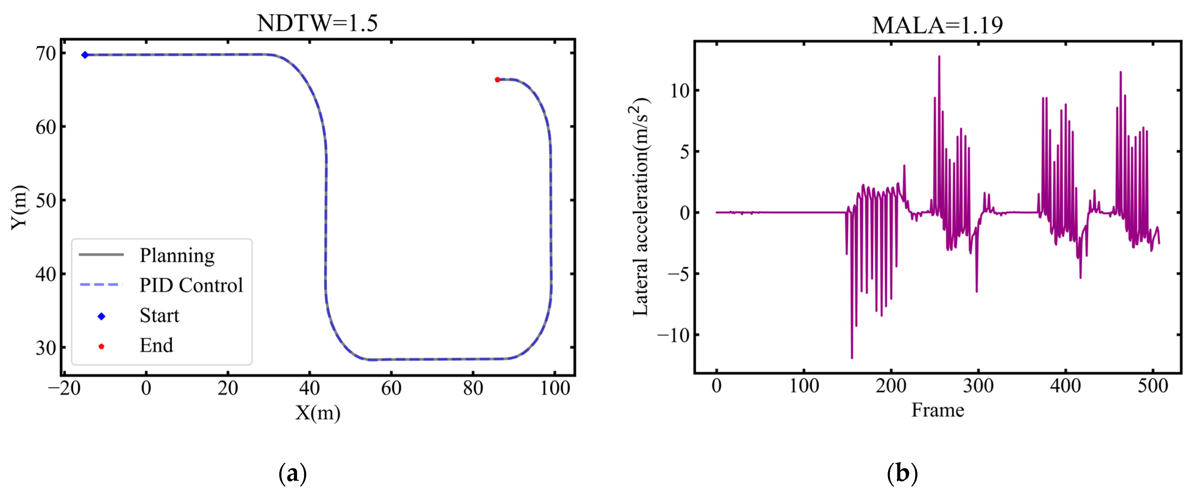
Finally, several representative yet challenging routes (as shown in Figure 15) are selected to evaluate the path-tracking performance. Obviously, Plan 2 obtained using DMEGO achieves excellent results both in terms of tracking accuracy and smoothness. Specifically, across a variety of routes encompassing straight segments, sharp turns, and lane changes, Plan 2 consistently achieves a trajectory (i.e., the blue dotted line) that precisely aligns with the global planning path (i.e., the gray solid line), which ensures the safety of the autonomous vehicle. In addition, even when encountering sharp turns, Plan 2 effectively maintains the lateral acceleration below 30 m / s 2 , thereby ensuring smooth operation and enhancing passenger comfort. In summary, the method proposed in this paper can obtain a set of robust and excellent PID parameters, which can be adapted to complex urban road environments.

5. Conclusions

In this paper, a novel simulation-based optimization method for AV path tracking was proposed. This method fully considers the complexity and uncertainty of the urban road environment and provides a robust solution for AV path tracking. This study develops a comprehensive simulation environment for AV path tracking, considering various environmental perturbations. Then, we present two evaluation indicators of tracking accuracy and smoothness and formulate the PID controller parameter optimization model under uncertainties. To solve this model, a simulation-based optimization algorithm named DMEGO is proposed and mainly includes three steps: (1) independently construct separate GP models for each objective function using evaluated observations; (2) employ the widely used NSGA-II algorithm to solve the maximization problem for the acquisition function and obtain a set of promising candidate solutions; (3) utilize the domination measure and the crowding distance to selectively retain a candidate solution exhibiting superior performance and good diversity for the next iteration. In the numerical experiments, the DMEGO algorithm is first tested using a stochastic FON function, and the numerical results validate the better performance of DMEGO compared with NSGA-II, ParEGO, and BOEGO. Finally, the proposed approach is applied to optimize the PID control parameters considering the complexity and uncertainty of urban roads. The numerical results show that the nondominated solutions from DMEGO perform well in terms of the tracking accuracy and smoothness under limited simulation budgets.
Future enhancements and directions will focus on the following aspects: (1) incorporating a parallel computing mechanism to evaluate multiple solutions concurrently, thereby reducing the computational time even further; (2) adopting a more advanced machine learning or deep learning model as the surrogate model and implementing batch selection strategies to enhance the algorithm performance; (3) exploring the application of reinforcement learning techniques to achieve online dynamic tuning of PID parameters; and (4) although all experiments in this paper were conducted in a simulator, it is crucial to evaluate the practical performance in real-world scenarios in the future.

Supplementary Materials

The following supporting information can be downloaded at https://www.mdpi.com/article/10.3390/math11234762/s1, Video S1: Performance demonstration of Plan 2 in autonomous driving path tracking.

Author Contributions

Y.C.: conceptualization, methodology, data curation, software, writing—original draft, visualization. F.Y.: Formal analysis, visualization, writing. All authors have read and agreed to the published version of the manuscript.

Funding

This research received no external funding.

Data Availability Statement

The data used in this paper will be made available upon request.

Acknowledgments

The authors want to thank Central South University for its support.

Conflicts of Interest

The authors declare that they have no known competing financial interest or personal relationships that could have appeared to influence the work reported in this paper.

References

  1. Van Brummelen, J.; O’Brien, M.; Gruyer, D.; Najjaran, H. Autonomous vehicle perception: The technology of today and tomorrow. Transp. Res. Part C Emerg. Technol. 2018, 89, 384–406. [Google Scholar] [CrossRef]
  2. Gong, B.; Xu, Z.; Wei, R.; Wang, T.; Lin, C.; Gao, P. Reinforcement Learning-Based Lane Change Decision for CAVs in Mixed Traffic Flow under Low Visibility Conditions. Mathematics 2023, 11, 1556. [Google Scholar] [CrossRef]
  3. Raouf, I.; Khan, A.; Khalid, S.; Sohail, M.; Azad, M.M.; Kim, H.S. Sensor-Based Prognostic Health Management of Advanced Driver Assistance System for Autonomous Vehicles: A Recent Survey. Mathematics 2022, 10, 3233. [Google Scholar] [CrossRef]
  4. Shang, W.-L.; Zhang, M.; Wu, G.; Yang, L.; Fang, S.; Ochieng, W. Estimation of traffic energy consumption based on macro-micro modelling with sparse data from Connected and Automated Vehicles. Appl. Energy 2023, 351, 121916. [Google Scholar] [CrossRef]
  5. Rana, M.M.; Hossain, K. Connected and autonomous vehicles and infrastructures: A literature review. Int. J. Pavement Res. Technol. 2023, 16, 264–284. [Google Scholar] [CrossRef]
  6. Wei, Y.; Zhang, J. A Vehicular Edge Computing-Based Architecture and Task Scheduling Scheme for Cooperative Perception in Autonomous Driving. Mathematics 2022, 10, 3328. [Google Scholar] [CrossRef]
  7. Chen, X.; Wang, Z.; Hua, Q.; Shang, W.L.; Luo, Q.; Yu, K. AI-Empowered Speed Extraction via Port-Like Videos for Vehicular Trajectory Analysis. IEEE Trans. Intell. Transp. Syst. 2023, 24, 4541–4552. [Google Scholar] [CrossRef]
  8. Schwarting, W.; Alonso-Mora, J.; Rus, D. Planning and decision-making for autonomous vehicles. Annu. Rev. Control Robot. Auton. Syst. 2018, 1, 187–210. [Google Scholar] [CrossRef]
  9. Kuutti, S.; Bowden, R.; Jin, Y.; Barber, P.; Fallah, S. A survey of deep learning applications to autonomous vehicle control. IEEE Trans. Intell. Transp. Syst. 2020, 22, 712–733. [Google Scholar] [CrossRef]
  10. Yang, L.; Zhan, J.; Shang, W.L.; Fang, S.; Wu, G.; Zhao, X.; Deveci, M. Multi-Lane Coordinated Control Strategy of Connected and Automated Vehicles for On-Ramp Merging Area Based on Cooperative Game. IEEE Trans. Intell. Transp. Syst. 2023, 24, 13448–13461. [Google Scholar] [CrossRef]
  11. Bi, H.; Shang, W.L.; Chen, Y.; Yu, K.; Ochieng, W.Y. An Incentive Based Road Traffic Control Mechanism for COVID-19 Pandemic Alike Emergency Preparedness and Response. IEEE Trans. Intell. Transp. Syst. 2022, 23, 25092–25105. [Google Scholar] [CrossRef]
  12. Viadero-Monasterio, F.; Nguyen, A.T.; Lauber, J.; Boada, M.J.L.; Boada, B.L. Event-Triggered Robust Path Tracking Control Considering Roll Stability Under Network-Induced Delays for Autonomous Vehicles. IEEE Trans. Intell. Transp. Syst. 2023, 1. [Google Scholar] [CrossRef]
  13. Zhou, X.; Wang, Z.; Shen, H.; Wang, J. Robust Adaptive Path-Tracking Control of Autonomous Ground Vehicles With Considerations of Steering System Backlash. IEEE Trans. Intell. Veh. 2022, 7, 315–325. [Google Scholar] [CrossRef]
  14. Jiang, K.; Hu, C.; Yan, F. Path-following control of autonomous ground vehicles based on input convex neural networks. Proc. Inst. Mech. Eng. Part D J. Automob. Eng. 2022, 236, 2806–2816. [Google Scholar] [CrossRef]
  15. Farag, W. Complex trajectory tracking using PID control for autonomous driving. Int. J. Intell. Transp. Syst. Res. 2020, 18, 356–366. [Google Scholar] [CrossRef]
  16. Lefevre, S.; Carvalho, A.; Borrelli, F. A learning-based framework for velocity control in autonomous driving. IEEE Trans. Autom. Sci. Eng. 2015, 13, 32–42. [Google Scholar] [CrossRef]
  17. Zhao, B.; Wang, H.; Li, Q.; Li, J.; Zhao, Y. PID trajectory tracking control of autonomous ground vehicle based on genetic algorithm. In Proceedings of the 2019 Chinese Control and Decision Conference (CCDC), Nanchang, China, 3–5 June 2019; pp. 3677–3682. [Google Scholar]
  18. Al-Mayyahi, A.; Wang, W.; Birch, P. Path tracking of autonomous ground vehicle based on fractional order PID controller optimized by PSO. In Proceedings of the 2015 IEEE 13th International Symposium on Applied Machine Intelligence and Informatics (SAMI), Herl’any, Slovakia, 22–24 January 2015; pp. 109–114. [Google Scholar]
  19. Abajo, M.R.; Sierra-García, J.E.; Santos, M. Evolutive tuning optimization of a PID controller for autonomous path-following robot. In Proceedings of the 16th International Conference on Soft Computing Models in Industrial and Environmental Applications (SOCO 2021), Bilbao, Spain, 22–24 September 2021; pp. 451–460. [Google Scholar]
  20. Gao, S.; Gao, S.; Pan, W.; Wang, M. Design of Improved PID Controller Based on PSO-GA Hybrid Optimization Algorithm in Vehicle Lateral Control. Stud. Inform. Control 2021, 30, 55–65. [Google Scholar] [CrossRef]
  21. El Hajjami, L.; Mellouli, E.M.; Berrada, M. Optimal PID control of an autonomous vehicle using Butterfly Optimization Algorithm BOA. In Proceedings of the 4th International Conference on Big Data and Internet of Things, Tangier-Tetuan, Morocco, 23–24 October 2019; pp. 1–5. [Google Scholar]
  22. Loucif, F.; Kechida, S.; Sebbagh, A. Whale optimizer algorithm to tune PID controller for the trajectory tracking control of robot manipulator. J. Braz. Soc. Mech. Sci. Eng. 2020, 42, 1. [Google Scholar] [CrossRef]
  23. Ma’ani, F.A.; Nazaruddin, Y.Y. Optimization of longitudinal control of an autonomous vehicle using flower pollination algorithm based on data-driven approach. Int. J. Sustain. Transp. Technol. 2020, 3, 58–65. [Google Scholar] [CrossRef]
  24. Nguyen, A.-T.; Reiter, S.; Rigo, P. A review on simulation-based optimization methods applied to building performance analysis. Appl. Energy 2014, 113, 1043–1058. [Google Scholar] [CrossRef]
  25. Bellamy, H.; Rehim, A.A.; Orhobor, O.I.; King, R. Batched bayesian optimization for drug design in noisy environments. J. Chem. Inf. Model. 2022, 62, 3970–3981. [Google Scholar] [CrossRef]
  26. Korovina, K.; Xu, S.; Kandasamy, K.; Neiswanger, W.; Poczos, B.; Schneider, J.; Xing, E. Chembo: Bayesian optimization of small organic molecules with synthesizable recommendations. In Proceedings of the Twenty Third International Conference on Artificial Intelligence and Statistics, Online, 26–28 August 2020; pp. 3393–3403. [Google Scholar]
  27. Zuo, Y.; Qin, M.; Chen, C.; Ye, W.; Li, X.; Luo, J.; Ong, S.P. Accelerating materials discovery with Bayesian optimization and graph deep learning. Mater. Today 2021, 51, 126–135. [Google Scholar] [CrossRef]
  28. Chen, Y.; Cheng, A.; Zhang, C.; Chen, S.; Ren, Z. Rapid mechanical evaluation of the engine hood based on machine learning. J. Braz. Soc. Mech. Sci. Eng. 2021, 43, 345. [Google Scholar] [CrossRef]
  29. Victoria, A.H.; Maragatham, G. Automatic tuning of hyperparameters using Bayesian optimization. Evol. Syst. 2021, 12, 217–223. [Google Scholar] [CrossRef]
  30. Močkus, J. On Bayesian methods for seeking the extremum. In Optimization Techniques IFIP Technical Conference; Springer: Berlin/Heidelberg, Germany, 1975; pp. 400–404. [Google Scholar]
  31. Jones, D.R.; Schonlau, M.; Welch, W.J. Efficient global optimization of expensive black-box functions. J. Glob. Optim. 1998, 13, 455–492. [Google Scholar] [CrossRef]
  32. Frazier, P.I. Bayesian optimization. In Recent Advances in Optimization and Modeling of Contemporary Problems; Informs: Catonsville, MA, USA, 2018; pp. 255–278. [Google Scholar]
  33. Hernández-Lobato, J.M.; Hoffman, M.W.; Ghahramani, Z. Predictive entropy search for efficient global optimization of black-box functions. Adv. Neural Inf. Process. Syst. 2014, 27. [Google Scholar]
  34. Liu, H.; Ong, Y.-S.; Cai, J. A survey of adaptive sampling for global metamodeling in support of simulation-based complex engineering design. Struct. Multidiscip. Optim. 2018, 57, 393–416. [Google Scholar] [CrossRef]
  35. Desautels, T.; Krause, A.; Burdick, J.W. Parallelizing exploration-exploitation tradeoffs in gaussian process bandit optimization. J. Mach. Learn. Res. 2014, 15, 3873–3923. [Google Scholar]
  36. González, J.; Dai, Z.; Hennig, P.; Lawrence, N. Batch Bayesian optimization via local penalization. In Proceedings of the 19th International Conference on Artificial Intelligence and Statistics, Cadiz, Spain, 9–11 May 2016; pp. 648–657. [Google Scholar]
  37. Knowles, J. ParEGO: A hybrid algorithm with on-line landscape approximation for expensive multiobjective optimization problems. IEEE Trans. Evol. Comput. 2006, 10, 50–66. [Google Scholar] [CrossRef]
  38. Emmerich, M.; Klinkenberg, J.-W. The Computation of the Expected Improvement in Dominated Hypervolume of Pareto Front Approximations; Rapport Technique; Leiden University: Leiden, The Netherlands, 2008; Volume 34, pp. 3–7. [Google Scholar]
  39. Picheny, V. Multiobjective optimization using Gaussian process emulators via stepwise uncertainty reduction. Stat. Comput. 2015, 25, 1265–1280. [Google Scholar] [CrossRef]
  40. He, X.; Chen, X.; Xiong, C.; Zhu, Z.; Zhang, L. Optimal Time-Varying Pricing for Toll Roads Under Multiple Objectives: A Simulation-Based Optimization Approach. Transp. Sci. 2016, 51, 412–426. [Google Scholar] [CrossRef]
  41. Rajamani, R. Vehicle Dynamics and Control; Springer Science & Business Media: Berlin, Germany, 2011. [Google Scholar]
  42. Dosovitskiy, A.; Ros, G.; Codevilla, F.; Lopez, A.; Koltun, V. CARLA: An open urban driving simulator. In Proceedings of the 1st Annual Conference on Robot Learning, Mountain View, CA, USA, 13–15 November 2017; pp. 1–16. [Google Scholar]
  43. Wang, S.; Lin, F.; Wang, T.; Zhao, Y.; Zang, L.; Deng, Y. Autonomous Vehicle Path Planning Based on Driver Characteristics Identification and Improved Artificial Potential Field. Actuators 2022, 11, 52. [Google Scholar] [CrossRef]
  44. Dechter, R.; Pearl, J. Generalized best-first search strategies and the optimality of A. J. ACM 1985, 32, 505–536. [Google Scholar] [CrossRef]
  45. Tao, Y.; Both, A.; Silveira, R.I.; Buchin, K.; Sijben, S.; Purves, R.S.; Laube, P.; Peng, D.; Toohey, K.; Duckham, M. A comparative analysis of trajectory similarity measures. GIScience Remote Sens. 2021, 58, 643–669. [Google Scholar] [CrossRef]
  46. Yu, Q.; Luo, Y.; Chen, C.; Chen, S. Trajectory similarity clustering based on multi-feature distance measurement. Appl. Intell. 2019, 49, 2315–2338. [Google Scholar] [CrossRef]
  47. Taylor, J.; Zhou, X.; Rouphail, N.M.; Porter, R.J. Method for investigating intradriver heterogeneity using vehicle trajectory data: A dynamic time warping approach. Transp. Res. Part B Methodol. 2015, 73, 59–80. [Google Scholar] [CrossRef]
  48. Wang, S.; Li, L.; Ma, W.; Chen, X. Trajectory analysis for on-demand services: A survey focusing on spatial-temporal demand and supply patterns. Transp. Res. Part C Emerg. Technol. 2019, 108, 74–99. [Google Scholar] [CrossRef]
  49. Matute-Peaspan, J.A.; Marcano, M.; Diaz, S.; Zubizarreta, A.; Perez, J. Lateral-Acceleration-Based Vehicle-Models-Blending for Automated Driving Controllers. Electronics 2020, 9, 1674. [Google Scholar] [CrossRef]
  50. Yamakado, M.; Abe, M. An experimentally confirmed driver longitudinal acceleration control model combined with vehicle lateral motion. Veh. Syst. Dyn. 2008, 46, 129–149. [Google Scholar] [CrossRef]
  51. Schulz, E.; Speekenbrink, M.; Krause, A. A tutorial on Gaussian process regression: Modelling, exploring, and exploiting functions. J. Math. Psychol. 2018, 85, 1–16. [Google Scholar] [CrossRef]
  52. Couckuyt, I.; Deschrijver, D.; Dhaene, T. Fast calculation of multiobjective probability of improvement and expected improvement criteria for Pareto optimization. J. Glob. Optim. 2014, 60, 575–594. [Google Scholar] [CrossRef]
  53. Zhan, D.; Xing, H. Expected improvement for expensive optimization: A review. J. Glob. Optim. 2020, 78, 507–544. [Google Scholar] [CrossRef]
  54. Garivier, A.; Moulines, E. On Upper-Confidence Bound Policies for Switching Bandit Problems. In Algorithmic Learning Theory; Springer: Berlin/Heidelberg, Germany, 2011; pp. 174–188. [Google Scholar]
  55. Hale, J.Q.; Zhu, H.; Zhou, E. Domination Measure: A New Metric for Solving Multiobjective Optimization. INFORMS J. Comput. 2020, 32, 565–581. [Google Scholar] [CrossRef]
  56. Mete, H.O.; Zabinsky, Z.B. Multiobjective Interacting Particle Algorithm for Global Optimization. INFORMS J. Comput. 2014, 26, 500–513. [Google Scholar] [CrossRef]
  57. Ishibuchi, H.; Imada, R.; Setoguchi, Y.; Nojima, Y. Reference point specification in inverted generational distance for triangular linear Pareto front. IEEE Trans. Evol. Comput. 2018, 22, 961–975. [Google Scholar] [CrossRef]
  58. Yan, J.; Li, C.; Wang, Z.; Deng, L.; Sun, D. Diversity Metrics in Multi-objective Optimization: Review and Perspective. In Proceedings of the 2007 IEEE International Conference on Integration Technology, Shenzhen, China, 20–24 March 2007; pp. 553–557. [Google Scholar]
  59. Fonseca, C.M.; Fleming, P.J. An overview of evolutionary algorithms in multiobjective optimization. Evol. Comput. 1995, 3, 1–16. [Google Scholar] [CrossRef]
  60. Deb, K.; Pratap, A.; Agarwal, S.; Meyarivan, T. A fast and elitist multiobjective genetic algorithm: NSGA-II. IEEE Trans. Evol. Comput. 2002, 6, 182–197. [Google Scholar] [CrossRef]
Figure 1. The result of the PID controller parameters by hand. Note: (a) represents the vehicle’s tracking trajectory, and (b) represents the lateral acceleration of the vehicle.
Mathematics 11 04762 g001
Figure 2. Bicycle vehicle dynamic model.
Mathematics 11 04762 g002
Figure 3. The illustration of the longitudinal and lateral PID controllers. Note: (a) denotes the control of the vehicle’s speed using the longitudinal controller, while (b) signifies the control of the vehicle’s direction using the lateral controller.
Mathematics 11 04762 g003
Figure 4. The proposed simulation environment for AV path tracking. (a) Sequence diagram for information synchronization among server, client, and hardware. (b) The detailed flow chart for AV path tracking in CARLA.
Mathematics 11 04762 g004
Figure 5. Illustration of two pairs of reference trajectory and query trajectory, and the optimal warping between them (black lines in (a,b)) obtained by computing NDTW.
Mathematics 11 04762 g005
Figure 6. Visualization of the GP posterior and EI function applied to a one-dimensional optimization problem. (a) and (b) represent the GP posterior and EI function after 1-th and 2-th iterations of the EGO algorithm, respectively.
Mathematics 11 04762 g006
Figure 7. Two objective functions and the Pareto optimal set for Example 1.
Mathematics 11 04762 g007
Figure 8. The rigorous quantification of the quality of a solution in Example 1 using (a) domination measure and (b) linear weighted sum method.
Mathematics 11 04762 g008
Figure 9. Convergence of DMEGO algorithm on problem (30). (a) n = 40, (b) n = 80, (c) n = 120, (d) n = 140, (e) n = 170, (f) n = 200.
Mathematics 11 04762 g009aMathematics 11 04762 g009b
Figure 10. Comparison of the nondominated solutions obtained using various algorithms.
Mathematics 11 04762 g010
Figure 11. Numerical results in term of (a) the iterative curve for IGD, (b) the iterative curve for Υ , and (c) the estimation errors of two GP models for bi-objective functions.
Mathematics 11 04762 g011
Figure 12. Optimization results for PID parameter optimization problem, where (a) represents all explored solutions in the objective space, (b) denotes the Pareto front, and (c) denotes the bi-objective values of the three nondominant solutions. Note: the gray pentagrams indicate 600 costly simulation evaluations, and the red, green, and blue circles depict three nondominated solutions.
Mathematics 11 04762 g012
Figure 13. Parallel coordinate plots of last 50 solutions for NDTW (a) and MALA (b).
Mathematics 11 04762 g013
Figure 14. A 3D visualization of our experimental scenarios. (a) Town 1, (b) Town 3, (c) Town 10, (d) light rain, (e) moderate rain, (f) heavy rain, (g) van, (h) car, (i) mini car.
Mathematics 11 04762 g014aMathematics 11 04762 g014b
Figure 15. The results of path tracking achieved by Plan 2. Note: (a,c,e,g) represent the vehicle’s tracking trajectory, and (b,d,f,h) represent the lateral acceleration of the vehicle.
Mathematics 11 04762 g015aMathematics 11 04762 g015b
Table 1. Summary of the PID parameter optimization work.
ReferenceEnvironmentVarious RoutesRoad SlopeWeatherVehicle TypeBi-ObjectiveOptimization Algorithm
[17]Mathematical modelGA
[18]MATLABPSO
[19]SimulinkGA
[20]MATLABPSO-GA
[21]SimulinkBOA
[22]SimulinkWOA
[23]CARLAFPA
Our workCARLADMEGO
Table 2. Environmental perturbations for path tracking.
Environmental PerturbationsExamples
TownMathematics 11 04762 i001
RoutesMathematics 11 04762 i002
Road slopeMathematics 11 04762 i003
Weather Mathematics 11 04762 i004
Vehicle typeMathematics 11 04762 i005
Table 3. Comparison results for four algorithms.
MethodFEsNSsIGD Υ
NSGA-II200160.10391.2068
ParEGO200260.03330.8328
BOEGO200610.01830.8029
DMEGO200980.00470.5079
Note: FEs refers to the number of function evaluations, while NSs represents the count of nondominated solutions.
Table 4. Three optimized plans obtained using the DMEGO method.
k p , l a t k i , l a t k d , l a t k p , l o n g k i , l o n g k d , l o n g
Plan 10.16362.53380.48784.13487.06271.9360
Plan 20.91191.64850.21560.46093.10662.1257
Plan 31.05811.09310.59951.55736.51036.7818
Disclaimer/Publisher’s Note: The statements, opinions and data contained in all publications are solely those of the individual author(s) and contributor(s) and not of MDPI and/or the editor(s). MDPI and/or the editor(s) disclaim responsibility for any injury to people or property resulting from any ideas, methods, instructions or products referred to in the content.