Abstract
This paper considers a dynamic Stackelberg game model for a manufacturer-led supply chain with risk aversion. Cooperative advertising strategy is applied to the marketing decisions of supply chain participants. Based on Stackelberg game and system dynamic theory, the game and complex dynamical behaviors are studied through the use of several methods, such as the stability region of the system, bifurcation diagram, attractor diagram, and the largest Lyapunov exponent diagram. The expected utilities of participants are given and compared by numerical simulation. The results illustrate that a series of variations in adjustment speed of advertising expenditure, participation rate of local advertising expenditure by manufacturer, risk tolerance levels, and the effect coefficient of advertising expenditure may cause a loss of stability to the system and evolve into chaos. Meanwhile, the Nash equilibrium point and the expected utility of the manufacturer and retailer will change greatly. The parameter control method is further applied to control the chaos phenomenon of the system effectively. By means of analyzing the impact of relevant factors on the game model, the manufacturer and retailer can make optimal strategy decisions in the supply chain competition. The findings of this study mainly include the following three aspects. Firstly, for market stability and maximizing revenue, the manufacturer adjusts the participation rate appropriately, avoiding too high or too low values. Secondly, the manufacturer will try to reduce their own risk tolerance level for the economic revenue, and the retailer appropriately adjust the risk tolerance level to adapt to their own development according to their own enterprise strategy. Finally, both the manufacturer and retailer reduce their own effect coefficients of advertising expenditure. Meanwhile, they will attempt to increase their opponent’s effect coefficient to gain the most revenue. The research results of this study can provide important reference for the advertising expenditure decision and revenue maximization of participants in the context of risk aversion.
Keywords:
manufacturer-led supply chain; cooperative advertising strategy; risk aversion; dynamic game; chaos MSC:
91-10
1. Introduction
Berger [1] first discussed cooperative advertising in a manufacturer–retailer channel, proposing a financing of advertising expenditures through a discount on the wholesale price by the retailer. Cooperative advertising is an interactive scheme in a supply chain system in which the manufacturer pays a part of the advertising expenditure incurred by the retailer in local advertisement. Fulop [2] considered that cooperative advertising was an important aspect of promotional activities by many manufacturers. Manufacturers can enhance brand image and boost sales through a cooperative advertising strategy. As distinguished by Bergen and John [3], advertising could be divided into national advertising and local advertising. For retailers, local advertising investment can attract potential customers to buy products. The goal of participating in the local advertising expenditure by the manufacturer is to influence the retailer to invest more, which can generate more sales [4,5].
The concept of risk management was first put forward by Nobel Prize winner Harry Markowitz in the 1950s [6] and later became a field of enterprise management. Early research on risk management mainly focused on the field of financial investment. Markowitz [7] was the first to introduce the statistical concepts of expectation and variance into the portfolio problem and used the variance of investment revenue as a measure of risk. Later, on this basis, many scholars put forward other financial risk measurement tools and extended them to inventory control, supply chain management, and other fields [8,9,10,11]. Previous literature on the supply chain considered that enterprises were risk-neutral. Early studies on supply chain models were usually based on the assumption of risk neutrality of decision makers, and the decision-making goals were generally to maximize expected profits or minimize expected costs. However, subsequent studies by experimental economist Marshall Fisher [12] showed that most decision makers were not risk-neutral. Anupindi and Bassok [13] pointed out that relaxation of the risk-neutral hypothesis would enable a better understanding of the behavior of supply chain decision makers. With the market uncertainty and intense competition, the ability of enterprises to take risks was seen as progressively affecting its overall revenue. Some enterprises preferred to sacrifice some revenue to avoid risk.
Researchers studied the effect of risk attitude on the decision-making behavior of the supply chain recently. In the field of enterprise management, most decision makers tended to be risk-averse [14,15,16]. Therefore, most scholars researched the decision-making issues of supply chains that consisted of one or more risk-averse participants. They mainly researched the effect of risk attitude on the production decisions, price decisions, and corporation strategy of supply chain participants. In the context of supply chain management, both the utility function approach and the mean-risk model had been widely applied to risk-averse decision-making problems [17]. Eeckhoudt and Gollier [8] explored the effect of risk attitude on decision making when they decided inventory levels without knowing market demand. Xiao and Yang [18] proposed the price service competition model of two supply chains. The study found that the higher the risk sensitivity of the retailer, the lower the optimal solution of service level and retail price. Zhang and Wang [19] mainly studied the coordination problem on dual channels of retailers in the case of short life cycles. With the increase of market demand uncertainty, enterprises must consider the risk tolerance of enterprises while pursuing the maximum profit. Therefore, the attitudes of enterprises towards risk affected the final profit of enterprises.
Beijing Automotive Industry Corporation (BAIC), which makes new energy vehicles, and vehicle retailers of Sale Service Sparepart and Survey (4S) constitute a typical manufacturer–retailer supply chain. Due to the impact of COVID-19, BAIC was faced with environmental risks, which posed a great risk to the stability of the entire supply chain. BAIC formulated rapid response strategies to improve the level of risk aversion and the risk management system for minimizing the impact of the sudden epidemic on the enterprises. By providing customers with a series of service-type advertising, including a sufficient supply of spare parts and timely tracking system, the 4S automobile retailers made customers trust the brand and expanded sales. In order to celebrate the cumulative sales volume of 100,000, BAIC cooperated with 15 retailers in Beijing, and then launched a special campaign for 10,000 people to buy cars as a reward to consumers. BAIC completed a reasonable share of the local advertising expenditure by retailers. The overall benefits of the supply chain were optimized.
Complexity theory was widely used to study the stability of various systems, such as mechanics, meteorology, economics, and supply chain systems. Based on bounded rational expectations, complexity theory discussed the characteristics of the system complexity produced by enterprise decision making, and analyzed the effect of dynamic adjustment on the supply chain. Ma and Wang [20] considered two non-cooperative game models using the bounded rational expectations theory. They found that the closed-loop supply chain system would be more likely to fall into chaos as the retailer’s position in the game increased. In addition, the decision-making stage of the decision-making body in the supply chain was a dynamic process. Based on this fact, many scholars introduced the nonlinear dynamics theory into the related problems of supply chain management and carried out a lot of research [21,22,23]. Sun and Ma [24] combined this with a pricing model of risk aversion in the supply chain and carried out the study of dynamic complexity by discussing the game process in the environment of incomplete information. Nonlinear dynamics was widely used as an effective tool theory and made a great impact in many research fields.
Combing the existing literature, this paper applies both risk aversion and cooperative advertising theory to the supply chain game model. Researchers consider a cooperative advertising supply chain as being composed of a manufacturer and a retailer which are both risk-averse participants. The research emphasis of this paper is the impact of the supply chain relevant factors, containing the adjustment speed of advertising expenditure, participation rate of local advertising expenditure by manufacturer, risk tolerance levels, and advertising expenditure effect coefficient. Based on the Stackelberg game model and system dynamic theory, this paper researches the effects of advertising investment and risk aversion on the stability of the supply chain and revenue of participants. There are three primary innovations in our paper. Firstly, researchers build a dynamical Stackelberg game model of cooperative advertising based on the supply chain with risk aversion. Secondly, effects of relevant factors such as adjustment speeds, risk tolerance levels, participation rate of manufacturer local advertising expenditure, and advertising expenditure effect coefficient are mainly analyzed on the stability and complex dynamic behavior of the supply chain. Thirdly, expected utilities of the participants are given and compared by the numerical simulation method that can provide guidance for the manufacturer and retailer to make optimal decisions.
The paper is organized as follows: Section 2 is a brief review of relevant studies. In Section 3, a Stackelberg supply chain game model is established and the equilibrium points and stability of the system are analyzed. In Section 4, the influences of relevant factors on complexity and expected utilities are given and compared by numerical simulation. In Section 5, system chaos control based on the parameter control method is investigated. Section 6 gives the conclusions of the paper.
2. Literature Review
Our research is mainly related to three streams of literature: cooperative advertising, risk aversion, and complexity in the supply chain. To highlight the contributions of the article, some representative literature examples are reviewed in these three streams.
2.1. Cooperative Advertising in Supply Chain
Cooperative advertising was extended by many authors under different settings [25,26]. Karray and Zaccour [27] demonstrated that cooperative advertising could also have harmful impacts on the retailers considering a bilateral duopoly. Xie and Wei [28] discussed coordinating advertising and pricing in a supply chain channel. Compared with the non-cooperative mode, the cooperative mode achieved better coordination by generating higher channel profits. The retailer price was lower to consumers and the advertising efforts were higher for all channel participants. Cooperative advertising was applied to the collaboration policy in supply chain management under uncertain conditions by Sarkar and Omair [29]. Through these research studies, it was concluded that the optimal decision of cooperative advertising made the revenue of the supply chain grow rapidly. Xiao and Zhou [30] established a mixed manufacturer–retailers advertising cooperation model, in which the manufacturer acted as the leading participant and played the Stackelberg game with the retailer coalition.
In recent years, more researchers have applied cooperative advertising to the supply chain and obtained a large amount of research results. Further research has shown that the investment of cooperative advertising affects the stability of the supply chain and the revenue of each participant.
2.2. Risk Aversion in Supply Chain
The crucial issue of supply chain risk management was risk measurement. The risk preference of participants had an important impact on the profit of each node enterprise and the whole supply chain. Therefore, more and more scholars began to study the influence of the risk preferences on production, price and profit, as well as on the coordination mechanism of conflicts among supply chain participants. Agrawal and Seshadri [31] demonstrated a single-cycle supply chain involving one supplier and multiple risk-averse retailers using a mean-variance approach. The research found that retailers could increase the number of orders to the expected optimal level and thus share the risk by offering reciprocal risk-sharing contracts. Xu and Dan [32] focused on the manufacturer’s dual-channel pricing strategy in a risk-averse supply chain. He found the price with risk aversion was lower than that with risk-neutral in a complete information environment of the dual-channel supply chain, and then proposed a two-way coordination mechanism of a profit-sharing contract. Yan and Jin [33] concentrated on the optimal decision-making problem of a supply chain with risk aversion under the condition of demand disturbance. Zhou and Li [34] built cooperative advertising and ordering in a two-level supply chain with risk aversion that considered manufacturers selling through retailers.
Based on the analysis of the literature, supply chain management with risk aversion has become a trending issue in the fields of economics and management. Researchers pay more attention to how participants effectively avoid risks in the competition so as to obtain maximum revenue.
2.3. Complexity in Supply Chain Game
In recent years, more researchers have applied game theory to study the system of the supply chain. However, the decision-making stage of the participants in the supply chain is a dynamic process. Based on this fact, nonlinear dynamics theory was introduced into related problems about supply chain management.
Karray and Amin [35] built a cooperative advertising model in a channel with competing retailers. The study discussed the equilibrium solution of the game model under centralized and decentralized decision making, and gave the corresponding coordination mechanism. The conclusion was that cooperative advertising stimulated retailers’ spending.
Based on game theory and chaotic dynamics theory, Ma and Ren [36] established a closed-loop supply chain model with dual recycling channels. The results show that a precipitous speeding of recycling price adjustment led the system into a chaotic state and caused the entropy of the system to increase. Ma and Hong [37] explored the dynamic game with risk attitudes and free ride. The pricing and service strategy were studied in a dual-channel supply chain. The study indicated that the system fell to chaos when the risk preference of the retailer was too high.
Stackelberg game theory was widely used in various fields of supply chain research as a conventional processing method of an economic model. Khademi and Ferrara [38] studied a two-level Stackelberg game model with two followers and a leader, and applied control theory and algorithm to obtain the optimal solution of the game model. This study was applicable to a long-term investment game model. Ma and Tian [39] constructed a long-term dynamic Stackelberg game model in three situations: without cap-and-trade regulation, grandfathering approach, and benchmarking approach. The work focused on the dynamic complexity study of a multi-channel supply chain which contained a manufacturer, an e-retailer, and a traditional retailer under cap-and-trade regulation.
Combing the previous literature, researchers find that most scholars established Stackelberg game models based on single risk aversion or cooperative advertising. Few scholars paid attention to research on the dynamic behavior of the Stackelberg game model in a cooperative advertising supply chain considering risk aversion. The influences of relevant factors on complexity and expected utilities of the supply chain were not studied and compared by numerical simulation.
3. Supply Chain Model
3.1. Model Description
In this research, researchers consider a supply chain which consists of a manufacturer and a retailer as shown in Figure 1. The manufacturer produces products and sells them to customers through the retailer. To improve sales volume, the manufacturer usually invests in national advertising and the retailer invests in local advertising. Considering the manufacturer as the leader deciding on national advertising investment and the retailer as the follower deciding on local advertising investment, researchers establish a Stackelberg game model of a manufacturer-led supply chain with risk-averse behavior.
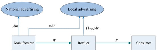
Figure 1.
The model framework.
Notations used throughout this paper are listed in Table 1.

Table 1.
Notations.
3.2. Model Assumption
The following assumptions are used for the game model of a manufacturer–retailer supply chain:
- (1)
- The unit production cost of the manufacturer and unit handling cost of the retailer incurred in addition to purchasing cost are assumed to be equal to zero.
- (2)
- Cooperative advertising is divided into the manufacturer’s national advertising expenditure and the retailer’s local advertising Due to different formula editors, some formula formats are not uniform. We will adjust the format of this part in later stage of production. , which are decision variables for the supply chain participants.
- (3)
- In this model, the manufacturer and retailer are risk-averse, which revenues are represented by exponential utility functions and follow a normal distribution.
3.3. Model Construction
The consumer demand function depends on the retail price and the advertising expenditures and , which is linear in prices and concave in advertising expenditure to account for decreasing marginal returns. This specification was widely used in previous research. The demand decreases in price and increases with advertising expenditures of the supply chain participants. The consumer demand function can be expressed as follows [35,40]:
The effect coefficients of advertising expenditure are captured by the positive parameters and . Parameter is the participation rate by the manufacturer, the percentage that the manufacturer agrees to pay the retailer to subsidize the local advertising expenditure. The profits of the manufacturer, the retailer, and the system are as follows, respectively [28]:
Parameter is a random variable, as follows . Here, is the mean of the baseline demand and follows a normal distribution, such that , , and . The exponential utility function is one form of the utility function, which dominates in both theoretical and applied study in the field of managerial decision making. Here, the manufacturer and retailer are risk-averse participants. The profit follows a normal distribution. Expected utility can been expressed by the following equation [37,41,42,43]:
This paper investigates the risk attitudes of the manufacturer and retailer, mainly referring to Xie and Yue [41] and Choi and Li [44]. Parameter is the risk tolerance level. The value of implies risk-averse behavior. When the value of is higher, the risk-averse degree is greater. When approaches 0, risk-neutral behavior is implied. Researchers can obtain the expected value and the variance value of the manufacturer and retailer as follows:
According to the Formulas (5)–(9), the expected utility function of the manufacturer and retailer can be expressed by the following equation:
From Formulas (10) and (11), researchers can obtain the revenue functions of the manufacturer and retailer which are more in accordance with the actual situation using the utility function. The prospects of the manufacturer and the retailer are to maximize respective expected utilities.
The manufacturer firstly determines advertising expenditure and the wholesale price of products. Based on the manufacturer’s decision information, the retailer determines advertising expenditure and the retail price of products. To solve the Stackelberg equilibrium, first consider the retailer’s optimal decisions [45].
The solutions can be solved by first order equations and .
Obtain the optimal values and :
Then, the expected utility function of the manufacturer has the form
Researchers can obtain , where and .
Then, can be obtained by Formulas (12) and (14):
In this paper, researchers develop a dynamic Stackelberg game model. Researchers assume that they adjust their advertising expenditures adaptively based on limited information and each enterprise can obtain its marginal utility information by means of market experiments [45]. In fact, when making advertising expenditure decisions, the manufacturer cannot obtain the whole market information, as they are restricted by the objective conditions such as the decision-making ability. Suppose that the decision in next period can be adjusted with bounded rationality based on partial estimation of marginal utility of the current period [46]. In each period, adjustments occur as follows: Firstly, manufacturer estimates marginal utility with respect to national advertising expenditure and makes decisions based on the bounded rational expectation. After the manufacturer carries out this decision, the retailer estimates the marginal utility with respect to local advertising expenditure according to the advertising expenditure of the manufacturer [45]. The model can be constructed as follows:
Here, and represent the advertising expenditure adjustment speed of the manufacturer and retailer, respectively.
3.4. The Stability of the System
In order to intuitively describe the dynamic competition process and complex system dynamics of enterprises, the numerical simulation is carried out in this section to investigate the influence of relevant parameters on system stability. Referring to related literature [5,41,47], the researchers used similar parameter settings for the numerical simulation. Based on satisfying constraints, we consider the assignment of relevant parameters.
The baseline demand should be large enough, so was assigned to be larger than other parameters. The researchers set as should be within . Other parameters were assigned as , , , , , and .
In system (18), let and . Then, researchers can obtain four groups of system equilibrium solutions as follows:
Obviously, , , and are partly or entirely zero. They are boundary unstable equilibrium points. is the unique non-negative equilibrium point of system (18). It is very significant to analyze the unique positive equilibrium point for participants. To study the local stability of equilibrium points, the Jacobian matrix at has the form
Its characteristic equation is , where is the trace and is the determinant of matrix , which are given by
Researchers can obtain . Thus, the eigenvalues of the Nash equilibrium are real. According to the Jury condition, the necessary and sufficient condition for the local stability of the Nash equilibrium can be obtained:
The long-term strategies of the manufacturer and retailer can remain stable when constraint (24) is satisfied. The above conditions are defined as the stability region of the adjustment parameters (,).
To study the influence of key parameters on the stability region of system (18), researchers examined a two-dimensional stable region with adjustment parameters (,) to examine the changing trend of the stable region when other parameters were fixed. If the values of (,) are in the stable region, the system will be stable at the Nash equilibrium after a number of games. The two-dimensional stable region of the system is presented in Figure 2 according to Equations (22)–(24).
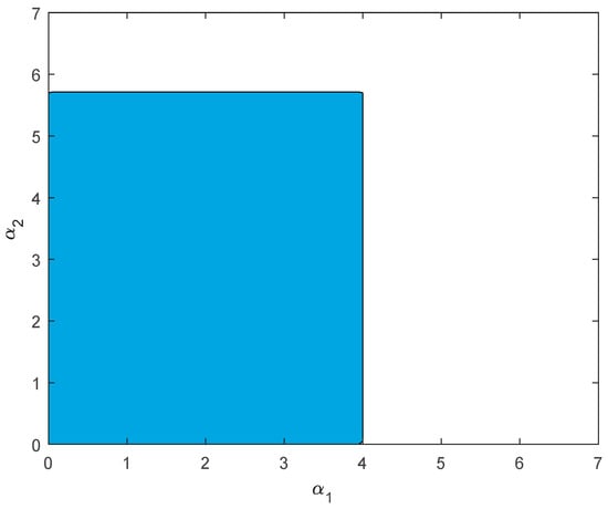
Figure 2.
The stable region of Nash Equilibrium in (, ) plane.
The blue areas indicate the stable region of the system and show the interaction effects between the adjustment parameters and . Obviously, the stable region is larger than . From the range of the stability region, researchers can see that the stability of the system is more sensitive to the manufacturer. If is relatively lower, even if is relatively higher, the system is stable, which also will be proved by the following figures. If the enterprises keep adjustment speeds (,) within the stability region, no matter what initial advertising expenditures are chosen by the enterprises, the market will eventually reach the Nash equilibrium after a series of games. As a result, the enterprises can obtain optimal strategies. Otherwise, complex phenomena such as bifurcation and chaos will appear.
The economic meaning of the stable region is that whatever initial values are chosen by the manufacturer and retailer in the local stable region, they will eventually achieve Nash equilibrium after finite games. Stability is beneficial for enterprises to make long-term strategies. Therefore, enterprises pay more attention to the stable region. The enterprises can forecast the development of the market but have to change their advertising expenditures frequently [48]. If the parameters exceed the stable region, the system will eventually be out of control and fall into chaos.
Based on the above reasons, researchers investigated the dynamics of system (18) and the impacts of relevant factors by means of dynamics analysis and numerical simulation, as described in the following sections. The complex dynamical behaviors of the system including the stable region, bifurcation, and chaos will be studied in detail.
4. Dynamics Analysis and Numerical Simulation
4.1. The Dynamics with Respect to Adjustment Speeds and
Dynamic characteristics can be expressed in the 2D bifurcation diagram [39]. In Figure 3, the light blue area stands for the stable region, while the bright blue, the dark blue, and the deep blue stand for the period-2, period-4, and period-8 stable regions. With the parameters and increasing continuously, the system will go into a chaos state. The chaos and divergence regions are shown by the gray and the white areas, respectively, which indicates that one enterprise will quit out of the market in economics. Figure 3 shows that has better stability than , illustrated by its larger stable region.
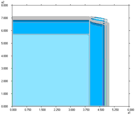
Figure 3.
Two-dimensional bifurcation diagram with respect to and .
Figure 4a,b show the bifurcation diagram of and with respect to . The corresponding largest Lyapunov exponent (LLE) is shown by Figure 4c,d, which is usually seen as characteristic value of chaos. It is shown that when the parameter , and become asymptotically stable with and . Researchers can observe that the stable region of is not changed with parameter . For , the system goes into period-2 bifurcation, which is improved by LLE from another aspect. After that, the system enters the 2-period state (), which also can be depicted by its attractor in Figure 5a,b. A further increase of will lead to the appearance of the period-4 state () and chaos (). Figure 5c,d show chaotic attractors with , which is consistent with Figure 4. Chaos attractors represent the disordered fluctuation of the system.
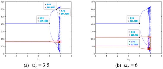
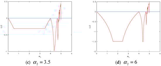
Figure 4.
The Bifurcation diagram and largest Lyapunov exponent with respect to .
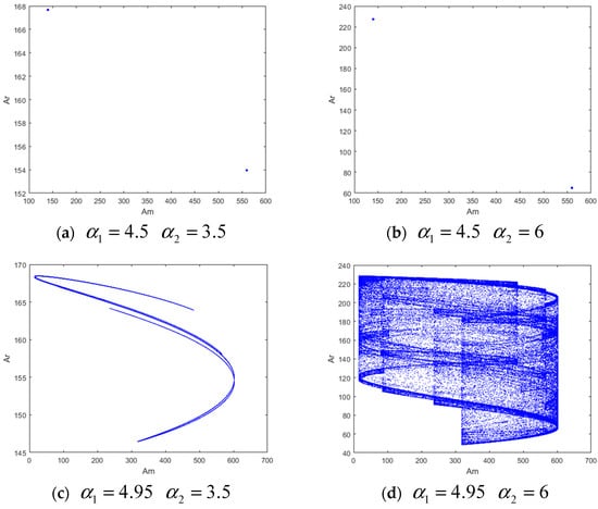
Figure 5.
The attractors of system with different and .
The corresponding Double Largest Lyapunov Exponents (DLLE) with respect to and are shown in Figure 6a,b. The blue areas are with a color transition from dark blue to light blue. When the LLE tends to 0, the color becomes light khaki and the system is in period-2 and period-4 stable cycles, etc. The dark khaki areas with the means the system is in chaos and divergence. Researchers can see the trend of system state from order to disorder by the perspective of LLE.
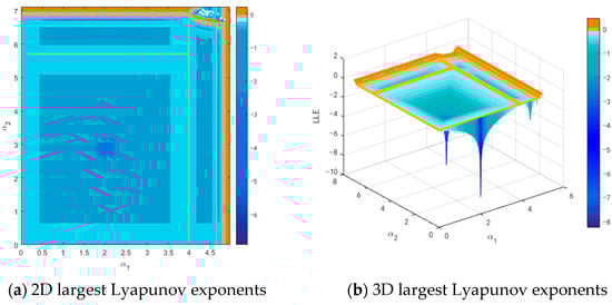
Figure 6.
The largest Lyapunov exponents with respect to and .
In the market, the objectives of the manufacturer and the retailer are to maximize respective expected utility. The effects of the parameters and on expected utilities and average expected utilities are shown in Figure 7. According to Figure 7a,b, when is in the stable region, expected utilities of the manufacturer and the retailer are stable at . With increasing, the system enters period-doubling bifurcation and a chaotic state. When and go into chaos, the oscillation of expected utilities intensifies, which has similar bifurcation properties to and .
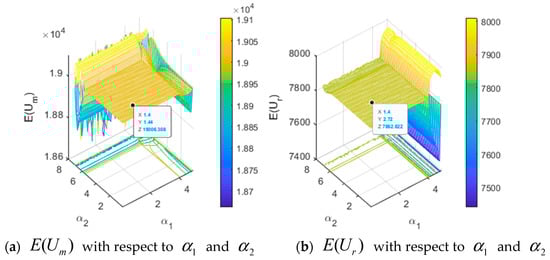
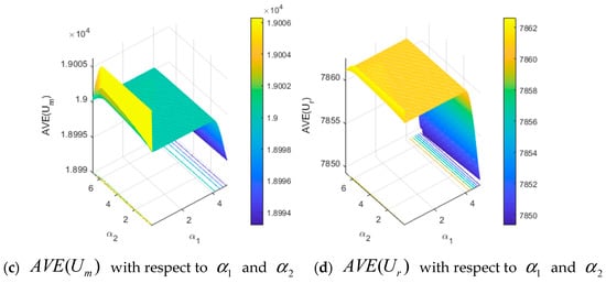
Figure 7.
The expected utilities and the average expected utilities with respect to and .
In Figure 7c,d, it can be found that the average expected utilities of the manufacturer and the retailer are in a downward state with the instability of the system. When the system loses the stability, the average expected utility will decrease, which is not in accord with the revenue of enterprises. It is favorable for participants to stabilize the system to the equilibrium point. Hence, the manufacturer and retailer will control their adjustment speed to maintain the stability of the market in order to obtain the maximum revenue.
4.2. The Influence of the Manufacturer Participation Rate
In this section, the influence of parameter on system stability and dynamic behavior will be studied.
Figure 8 clearly indicates the 2D bifurcation diagrams of the system with , respectively. From the 2D bifurcation diagrams, researchers can clearly know that different bifurcation curves correspond to different values of parameter . Researchers can find that rarely has influence on the stable region of . However, has a greater influence on the stable region of , which becomes larger with a greater . This indicates that the participation rate of local advertising by the manufacturer has a positive impact on the system’s stability, that is, the higher the degree of the manufacturer’s participation rate, the harder for the Nash equilibrium point to lose its stability.
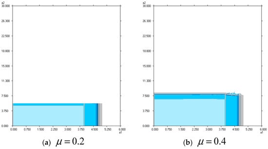
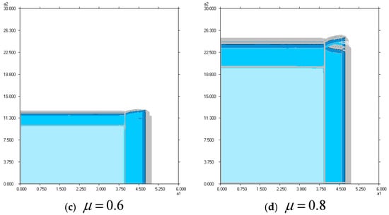
Figure 8.
The 2D bifurcation diagrams with respect to and with different .
Figure 9 shows the bifurcation diagram of and with respect to when the system is stable, during period-2 bifurcation, period-4 bifurcation, and chaos, respectively, with and taking different values. Researchers can see that decreases slightly, but increases dramatically as increases. Therefore, the greater the participation rate in local advertising by the manufacturer, the more the retailer spends on the local advertising expenditure. However, the manufacturer’s national advertising expenditure only has a slight downward adjustment with the increase of participation rate .
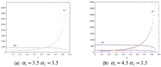
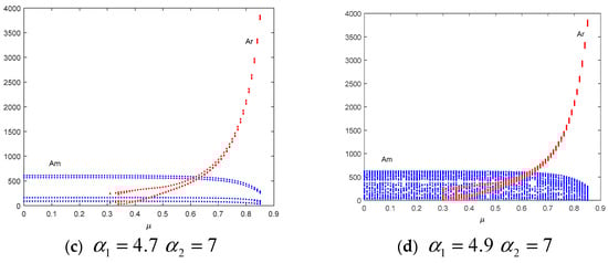
Figure 9.
The Bifurcation diagram of and with respect to with different and .
The expected utilities of manufacturer and retailer are shown in Figure 10. With the increase in participation rate and the change of system state, the manufacturer’s expected utility decreases, while the retailer’s expected utility increases slightly on the whole. Therefore, in real market competition, the manufacturer tries to avoid taking too large a value of the participation rate for obtaining the maximum expected utility. Although the retailer will obtain more expected utility by increasing , it will also increase local advertising expenditure rapidly. In order to maintain market stability and maximize revenue for both participants, as the dominant enterprise in the market, the manufacturer will adjust the participation rate appropriately, neither too high nor too low.
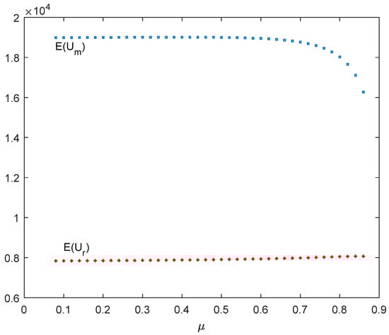
Figure 10.
The expected utilities with respect to with and .
4.3. The Influence of Risk Tolerance Levels and
In this section, the influence of risk tolerance levels and is to be analyzed with respect to the Nash equilibrium point and expected utilities.
In order to analyze the effects of risk tolerance levels on the stable region, the corresponding 2D bifurcation diagrams are shown in Figure 11. Researchers chose as , , , and , respectively, and other parameters remained unchanged as in system (18). Researchers can find that the stable region has no variation with risk tolerance levels and .
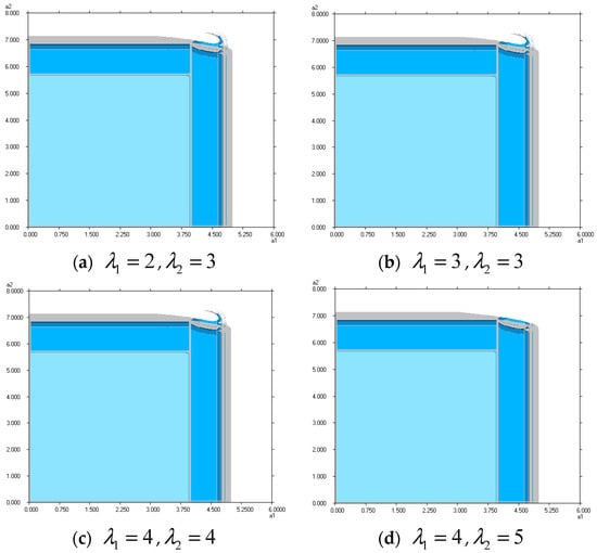
Figure 11.
The 2D bifurcation diagram with respect to and with different and .
Figure 12a,b are the 3D bifurcation diagrams with respect to the parameters , , and , , , respectively. Figure 12c,d are the 3D bifurcation diagrams with the parameters , , and , , , respectively. Researchers can find that the Nash equilibrium of the system does not change with risk tolerance levels . Figure 12c,d show the change of Nash equilibrium is very slight, whereas Nash equilibrium is obvious with risk tolerance levels .
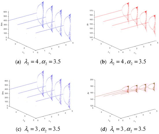
Figure 12.
The 3D bifurcation diagrams of and with respect to with (a,b) and (c,d) .
Figure 13 shows the Nash equilibrium points of and with respect to and . Figure 13a,b indicate the influence of risk tolerance level and on advertising expenditures and , respectively, when the system is in a stable state. The expected utilities of the manufacturer and retailer with respect to and are described by Figure 13c,d. In order to compare the Nash equilibrium and expected utilities with different values of and more clearly, Table 2 has been created with respect to and with and . Researchers can conclude that
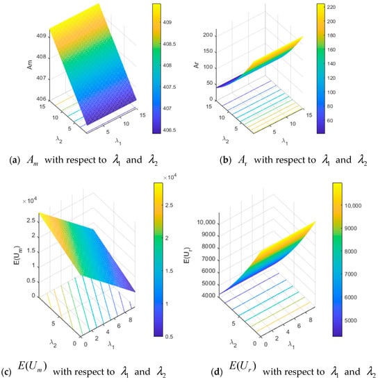
Figure 13.
Nash equilibrium points and the expected utilities with .
Table 2.
Nash equilibrium points and expected utilities with respect to and with and .
(1) The Nash equilibrium rises slightly and reduces with increasing risk tolerance level , while and remain unchanged with an increase in risk tolerance level , which corresponds to Figure 13a,b. Therefore, the retailer will try to increase their own risk tolerance level for less local advertising expenditure.
(2) The expected utility decreases and remains unchanged with an increase in risk tolerance level . The expected utility increases and decreases with an increase in risk tolerance level . These correspond to Figure 13c,d. Therefore, in order to obtain more expected utilities, the manufacturer and retailer will try to reduce their own risk tolerance levels. Meanwhile, the manufacturer wants to increase the risk tolerance level of retailer for its own revenue.
4.4. The Influence of Advertising Expenditure Effect Coefficients and
In this section, the influence of effect coefficients and is to be analyzed with respect to the Nash equilibrium point and expected utilities.
The 2D bifurcation diagrams are shown in Figure 14. Researchers can find that the stable region has no variation when effect coefficients are , , , and , respectively. No matter how and change, the system stability remains fixed with and .
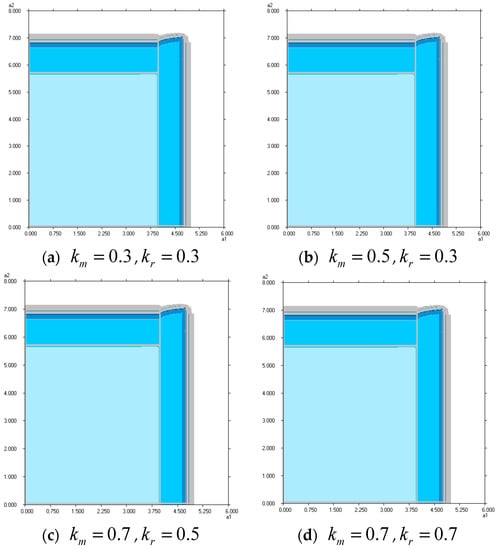
Figure 14.
The 2D bifurcation diagram with respect to and with different and .
Figure 15a,b are the 3D bifurcation diagrams with respect to the parameters , , and , , , respectively. Figure 15c,d are the 3D bifurcation diagrams with the parameters , , and , , , respectively. Researchers can find that the Nash equilibrium is changed with effect coefficients and . As shown in Figure 15a,b, the values of the Nash equilibrium increase with the increase in . As shown in Figure 15c,d, the increase in can increase the values of the Nash equilibrium . Meanwhile, the bifurcations and the chaos of the system are indicated clearly.
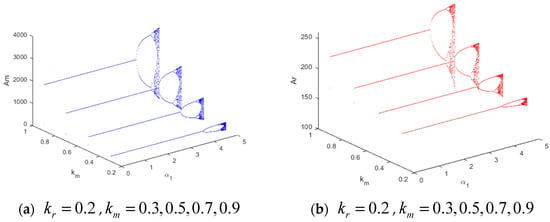
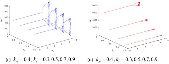
Figure 15.
The 3D bifurcation diagrams of and with respect to with .
Figure 16 shows the Nash equilibrium points of and with respect to and . Figure 16a,b indicate the influence of effect coefficients and on advertising expenditures and when the system is stable. Figure 16c,d describe the expected utilities of the manufacturer and retailer with respect to and . In order to compare the Nash equilibrium and expected utilities more clearly, the following Table 3 was created with respect to and with and . By comparison, researchers can find that
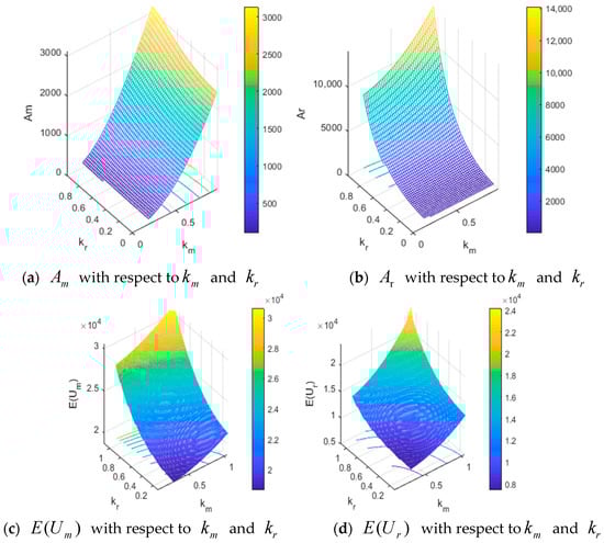
Figure 16.
Nash equilibrium points and the expected utilities with .
Table 3.
Nash equilibrium points and expected utilities with respect to and with and .
(1) With an increase in effect coefficients and , the stable region remains unchanged.
(2) The Nash equilibrium and rise with an increase in effect coefficients and . grows rapidly but slowly and relative to the increase in , meanwhile grows slowly but rapidly relative to the increase in . Researchers can see from the trend of the graph in Figure 16a,b that and are greatly influenced by and , respectively. Therefore, the manufacturer and retailer will try to reduce their own effect coefficients and for less advertising expenditures. More noteworthy is that the increase in their effect coefficient has a greater impact on their own advertising investment.
(3) The expected utilities and rise with an increase in effect coefficients and . The expected utility grows slowly with an increase in ; meanwhile, growth is rapid relative to an increase in . Researchers can also see from the trend of the graph in Figure 16c that the expected utility grows slowly with an increase in ; meanwhile, growth is rapid relative to an increase in . These correspond to Figure 16d. The effect coefficient of the opponent has a greater impact on its own expected utility. Therefore, in order to obtain more expected utilities and less advertising expenditures, while decreasing their own effect coefficient, the manufacturer and retailer will be willing to increase the opponent’s effect coefficient to gain the most revenue.
5. Chaos Control
Based on the discussion above, the chaotic state frequently appears against the stability of the supply chain, which is harmful to market returns. The manufacturer and retailer in the supply chain try their best to take measures to prevent the period-doubling bifurcation and chaotic state.
Referring to previous studies, the parameters control method is used to control chaos. Here, set the control parameter [33,49,50,51]. The manufacturer and retailer should control their adjustment speed of relevant variables when they formulate a management strategy. The system (18) can be rewritten as:
Figure 17 shows the bifurcation and LLE diagram with respect to parameter with and . The system changes from chaos to stability when parameter is . returns to Nash equilibrium with an increase in parameter .
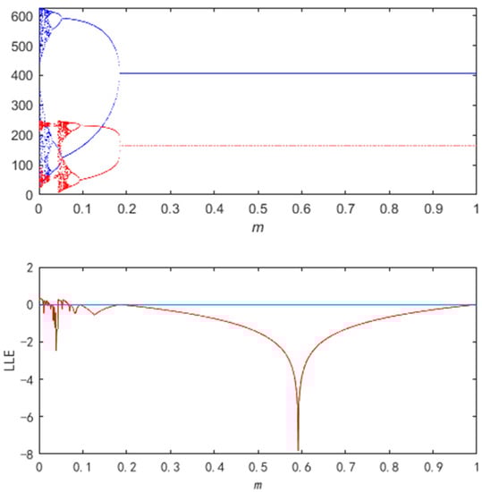
Figure 17.
The bifurcation diagram of and and the largest Lyapunov exponent with respect to .
Through comparison between the stable regions in Figure 18, researchers can find that the range of the stable region is extended compared with the one without chaos control in Figure 3. By , the stable region expands with an increase in parameter . Nevertheless, the Nash equilibrium does not change with parameter and stays at .
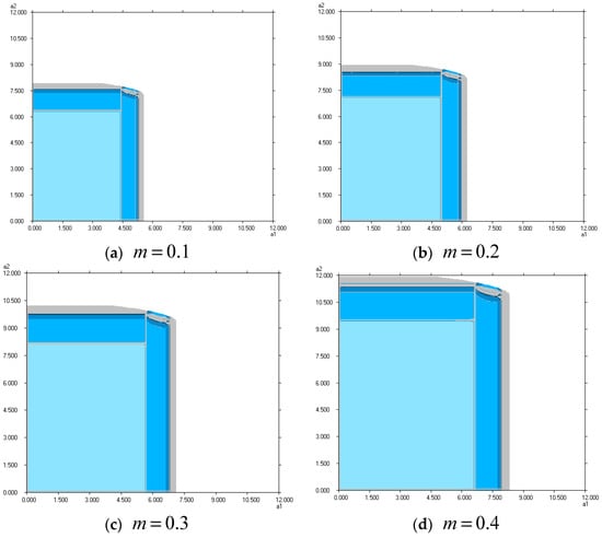
Figure 18.
The 2D bifurcation diagrams with respect to and with different .
6. Contribution and Implication
The major findings obtained in this paper can be employed by managers of supply chains as follows:
- (1)
- If the enterprises keep adjustment speeds within the stability region, no matter what initial advertising expenditures are chosen by the enterprises, the market will eventually reach the Nash equilibrium after a series of games. As a result, the enterprises can obtain optimal strategies. Otherwise, if the adjustment speeds of advertising expenditure are too fast, the system loses stability and enters chaotic states, which lead to a rapid decrease in expected utilities. The manufacturer and retailer will control their adjustment speeds to maintain the stability of the supply chain market for the maximum revenue.
- (2)
- The stability range of the system expands with an increase in the participation rate of local advertising expenditure by the manufacturer. As the manufacturer increases the participation rate of local advertising, the retailer spends more on local advertising expenditures. However, the national advertising expenditure of the manufacturer only has a slight downward adjustment with the increase in the participation rate. The expected utility of the manufacturer decreases, while the retailer increases slightly on the whole by an increase in the participation rate. For market stability and maximizing revenue, the manufacturer should adjust the participation rate appropriately, avoiding too high or too low values.
- (3)
- The stable region has no variation with risk tolerance levels of the manufacturer and retailer. The risk tolerance level of the manufacturer has no effect on the national advertising expenditure by the manufacturer and local advertising expenditure by the retailer. However, the manufacturer’s national advertising expenditure rises and the retailer’s local advertising expenditure reduces with an increase in the risk tolerance level of the retailer when the system is in a stable state. The expected utility of the manufacturer decreases and the expected utility of retailer remains unchanged with an increase in the risk tolerance level of the manufacturer. The expected utility of the manufacturer rises and the expected utility of the retailer decreases with an increase in the risk tolerance level of the retailer. Hence, the manufacturer will try to reduce their own risk tolerance level for economic revenue. In order to make neither too much advertising expenditure nor too little expected utility, the retailer will appropriately adjust the risk tolerance level to adapt to their own development according to their own enterprise strategy in the supply chain market competition.
- (4)
- With increasing effect coefficients of advertising expenditure, the stable region remains unchanged. The advertising expenditures and expected utilities rise with an increase in effect coefficients of advertising expenditure. The increase in its effect coefficient has a greater impact on its own advertising investment. In order to obtain more expected utilities and less advertising expenditures, both the manufacturer and retailer will reduce their own effect coefficients of advertising expenditure; meanwhile, they will attempt to increase their opponent’s effect coefficients to gain the most revenue.
- (5)
- It is profitable to keep the relevant factors in a certain range for manufacturer and retailer. Once the system falls into chaos, the chaos phenomenon can be delayed or eliminated effectively by the parameters control method.
Some valuable managerial implications for managers are summarized as follows: First, the appropriate participation rate of local advertising expenditure not only is good for the revenue of participants, but also is conducive to the stability of the supply chain, which needs to be constantly adjusted by the manufacturer in the competitive supply chain market. Second, the manufacturer and retailer will try to reduce their own risk tolerance levels for economic revenue, which makes it impossible for enterprises to avoid risks. However, in the realistic market competition, enterprises need to avoid risks as much as possible to ensure the stability of the market, avoiding market turbulence. Therefore, enterprises cannot develop steadily for a long time in the fierce supply chain market competition. Finally, once the market is in a chaotic state, the control method is applied by the manager effectively to avoid some loss in revenue.
7. Conclusions
In this paper, considering cooperative advertising, researchers have established a Stackelberg dynamic game model of a manufacturer–retailer supply chain with risk-averse behavior. Based on game and dynamics theory, the influence of relevant parameters on the stability of the model has been researched. The impact of adjustment speeds, risk tolerance levels, participation rate of local advertising expenditure by the manufacturer, and effect coefficients of advertising expenditure on system complexity and expected utilities have been analyzed by the numerical simulation method. Based on the parameters control method, the chaotic state of the system is effectively controlled. The research results of this study can provide important reference for advertising expenditure decisions and revenue maximization of participants in the context of risk aversion.
There are still some limitations in the paper. The analysis of the Stackelberg dynamic game model of the manufacturer and retailer might be simple in practice. The future work can consider a complicated multi-channel supply chain game model with a combination of traditional and online factors, and take into account the impact of more factors on the multi-channel supply chain stability, including but not limited to risk aversion and cooperative advertising.
Author Contributions
Writing—original draft, J.L.; Funding acquisition, C.L. All authors have read and agreed to the published version of the manuscript.
Funding
This work is supported by the National Natural Science Foundation of China (No. 71673042).
Data Availability Statement
Not applicable.
Acknowledgments
The authors are grateful to the reviewers and associate editor for their extremely useful comments.
Conflicts of Interest
The authors declare no conflict of interest regarding the publication of this paper.
References
- Berger, P.D. Vertical Cooperative Advertising Ventures. J. Mark. Res. 1972, 9, 309–312. [Google Scholar] [CrossRef]
- Fulop, C. The Role of Advertising in the Retail Marketing Mix. Int. J. Advert. 1988, 7, 99–117. [Google Scholar] [CrossRef]
- Bergen, M.; John, G. Understanding Cooperative Advertising Participation Rates in Conventional Channels. J. Mark. Res. 1997, 34, 357–369. [Google Scholar] [CrossRef]
- Zhang, J.; Gou, Q.; Liang, L.; Huang, Z. Supply chain coordination through cooperative advertising with reference price effect. Omega 2013, 41, 345–353. [Google Scholar] [CrossRef]
- Giri, B.C.; Sharma, S. Manufacturer’s pricing strategy in a two-level supply chain with competing retailers and advertising cost dependent demand. Econ. Model. 2014, 38, 102–111. [Google Scholar] [CrossRef]
- Stuart, A. Portfolio Selection: Efficient Diversification of Investment. OR 1959, 10, 253–254. [Google Scholar] [CrossRef]
- Markowitz, H.M. Portfolio Selection: Efficient Diversification of Investments; Wiley: New York, NY, USA, 1959. [Google Scholar]
- Eeckhoudt, L.; Gollier, C.; Schlesinger, H. The Risk-Averse (and Prudent) Newsboy. Manag. Sci. 1995, 41, 786–794. [Google Scholar] [CrossRef]
- Martínez-de-Albéniz, V.; Simchi-Levi, D. Mean-variance trade-offs in supply contracts. Nav. Res. Logist. 2006, 53, 603–616. [Google Scholar] [CrossRef]
- Kahneman, D.; Tversky, A. Prospect Theory: An Analysis of Decision under Risk. Econometrica 1979, 47, 263–291. [Google Scholar] [CrossRef]
- Zhao, H.; Wang, H.; Liu, W.; Song, S.; Liao, Y. Supply Chain Coordination with a Risk-Averse Retailer and the Call Option Contract in the Presence of a Service Requirement. Mathematics 2021, 9, 787. [Google Scholar] [CrossRef]
- Marshall Fisher, A.R. Reducing the Cost of Demand Uncertainty Through Accurate Response to Early Sales. Oper. Res. 1996, 44, 87–99. [Google Scholar] [CrossRef]
- Anupindi, R.; Bassok, Y. Centralization of stocks: Retailers vs. manufacturer. Manag. Sci. 1999, 45, 178–191. [Google Scholar] [CrossRef]
- Gan, X.; Sethi, S.P.; Yan, H. Channel Coordination with a Risk-Neutral Supplier and a Downside-Risk-Averse Retailer. Prod. Oper. Manag. 2005, 14, 80–89. [Google Scholar] [CrossRef]
- Rockafellar, R.T.; Uryasev, S. Conditional value-at-risk for general loss distributions. J. Bank. Financ. 2002, 26, 1443–1471. [Google Scholar] [CrossRef]
- Gao, T.; Wang, K.; Mei, Y.; He, S.; Wang, Y. Supply Chain Pricing Models Considering Risk Attitudes under Free-Riding Behavior. Mathematics 2022, 10, 1723. [Google Scholar] [CrossRef]
- Choi, T.-M.; Ma, C.; Shen, B.; Sun, Q. Optimal pricing in mass customization supply chains with risk-averse agents and retail competition. Omega 2019, 88, 150–161. [Google Scholar] [CrossRef]
- Xiao, T.; Yang, D. Price and service competition of supply chains with risk-averse retailers under demand uncertainty. Int. J. Prod. Econ. 2008, 114, 187–200. [Google Scholar] [CrossRef]
- Zhang, L.; Wang, J. Coordination of the traditional and the online channels for a short-life-cycle product. Eur. J. Oper. Res. 2017, 258, 639–651. [Google Scholar] [CrossRef]
- Ma, J.; Wang, H. Complexity analysis of dynamic noncooperative game models for closed-loop supply chain with product recovery. Appl. Math. Model. 2014, 38, 5562–5572. [Google Scholar] [CrossRef]
- Liu, J.; Liu, G.; Li, N.; Xu, H. Dynamics Analysis of Game and Chaotic Control in the Chinese Fixed Broadband Telecom Market. Discret. Dyn. Nat. Soc. 2014, 2014, 275123. [Google Scholar] [CrossRef]
- Askar, S.S.; Al-Khedhairi, A. Local and Global Dynamics of a Constraint Profit Maximization for Bischi–Naimzada Competition Duopoly Game. Mathematics 2020, 8, 1458. [Google Scholar] [CrossRef]
- Askar, S.S. The Influences of Asymmetric Market Information on the Dynamics of Duopoly Game. Mathematics 2020, 8, 1132. [Google Scholar] [CrossRef]
- Sun, L.; Ma, J. Study and Simulation on Dynamics of a Risk-Averse Supply Chain Pricing Model with Dual-Channel and Incomplete Information. Int. J. Bifurc. Chaos 2016, 26, 1650146. [Google Scholar] [CrossRef]
- Berger, P.D.; Magliozzi, T. Optimal Co-Operative Advertising Decisions in Direct-Mail Operations. J. Oper. Res. Soc. 1992, 43, 1079–1086. [Google Scholar] [CrossRef]
- Dant, R.P.; Berger, P.D. Modelling Cooperative Advertising Decisions in Franchising. J. Oper. Res. Soc. 1996, 47, 1120–1136. [Google Scholar] [CrossRef]
- Karray, S.; Zaccour, G. Could co-op advertising be a manufacturer’s counterstrategy to store brands? J. Bus. Res. 2006, 59, 1008–1015. [Google Scholar] [CrossRef]
- Xie, J.; Wei, J.C. Coordinating advertising and pricing in a manufacturer–retailer channel. Eur. J. Oper. Res. 2009, 197, 785–791. [Google Scholar] [CrossRef]
- Sarkar, B.; Omair, M.; Kim, N. A cooperative advertising collaboration policy in supply chain management under uncertain conditions. Appl. Soft Comput. 2020, 88, 105948. [Google Scholar] [CrossRef]
- Xiao, D.; Zhou, Y.-W.; Zhong, Y.; Xie, W. Optimal cooperative advertising and ordering policies for a two-echelon supply chain. Comput. Ind. Eng. 2019, 127, 511–519. [Google Scholar] [CrossRef]
- Agrawal, V.; Seshadri, S. Impact of Uncertainty and Risk Aversion on Price and Order Quantity in the Newsvendor Problem. Manuf. Serv. Oper. Manag. 2000, 2, 410–423. [Google Scholar] [CrossRef]
- Xu, G.; Dan, B.; Zhang, X.; Liu, C. Coordinating a dual-channel supply chain with risk-averse under a two-way revenue sharing contract. Int. J. Prod. Econ. 2014, 147, 171–179. [Google Scholar] [CrossRef]
- Yan, B.; Jin, Z.; Liu, Y.; Yang, J. Decision on risk-averse dual-channel supply chain under demand disruption. Commun. Nonlinear Sci. Numer. Simul. 2018, 55, 206–224. [Google Scholar] [CrossRef]
- Zhou, Y.-W.; Li, J.; Zhong, Y. Cooperative advertising and ordering policies in a two-echelon supply chain with risk-averse agents. Omega 2018, 75, 97–117. [Google Scholar] [CrossRef]
- Karray, S.; Amin, S.H. Cooperative advertising in a supply chain with retail competition. Int. J. Prod. Res. 2014, 53, 88–105. [Google Scholar] [CrossRef]
- Ma, J.; Ren, H.; Yu, M.; Zhu, M. Research on the Complexity and Chaos Control about a Closed-Loop Supply Chain with Dual-Channel Recycling and Uncertain Consumer Perception. Complexity 2018, 2018, 9853635. [Google Scholar] [CrossRef]
- Ma, J.; Hong, Y. Dynamic game analysis on pricing and service strategy in a retailer-led supply chain with risk attitudes and free-ride effect. Kybernetes 2021, 51, 1199–1230. [Google Scholar] [CrossRef]
- Khademi, M.; Ferrara, M.; Pansera, B.; Salimi, M. A dynamic game on Green Supply Chain Management. arXiv 2015, arXiv:1503.04772. [Google Scholar]
- Ma, J.; Tian, Y.; Xu, T.; Koivumäki, T.; Xu, Y. Dynamic game study of multi-channel supply chain under cap-and-trade regulation. Chaos Solitons Fractals 2022, 160, 112131. [Google Scholar] [CrossRef]
- Karray, S. Periodicity of pricing and marketing efforts in a distribution channel. Eur. J. Oper. Res. 2013, 228, 635–647. [Google Scholar] [CrossRef]
- Xie, G.; Yue, W.; Wang, S.; Lai, K.K. Quality investment and price decision in a risk-averse supply chain. Eur. J. Oper. Res. 2011, 214, 403–410. [Google Scholar] [CrossRef]
- Walls, M.R. Combining decision analysis and portfolio management to improve project selection in the exploration and production firm. J. Pet. Sci. Eng. 2004, 44, 55–65. [Google Scholar] [CrossRef]
- Avinadav, T.; Chernonog, T.; Perlman, Y. Mergers and acquisitions between risk-averse parties. Eur. J. Oper. Res. 2017, 259, 926–934. [Google Scholar] [CrossRef]
- Choi, T.-M.; Li, D.; Yan, H. Mean–variance analysis of a single supplier and retailer supply chain under a returns policy. Eur. J. Oper. Res. 2008, 184, 356–376. [Google Scholar] [CrossRef]
- Guo, Z.; Ma, J. Dynamics and implications on a cooperative advertising model in the supply chain. Commun. Nonlinear Sci. Numer. Simul. 2018, 64, 198–212. [Google Scholar] [CrossRef]
- Li, T.; Ma, J. Complexity analysis of dual-channel game model with different managers’ business objectives. Commun. Nonlinear Sci. Numer. Simul. 2015, 20, 199–208. [Google Scholar] [CrossRef]
- Ma, J.; Li, Q.; Bao, B. Study on Complex Advertising and Price Competition Dual-Channel Supply Chain Models Considering the Overconfidence Manufacturer. Math. Probl. Eng. 2016, 2016, 2027146. [Google Scholar] [CrossRef]
- Ma, J.; Guo, Z. The influence of information on the stability of a dynamic Bertrand game. Commun. Nonlinear Sci. Numer. Simul. 2016, 30, 32–44. [Google Scholar] [CrossRef]
- Xi, X.; Zhang, Y. Complexity analysis of production, fertilizer-saving level, and emission reduction efforts decisions in a two-parallel agricultural product supply chain. Chaos Solitons Fractals 2021, 152, 111358. [Google Scholar] [CrossRef]
- Tian, Y.; Ma, J.; Xie, L.; Koivumäki, T.; Seppänen, V. Coordination and control of multi-channel supply chain driven by consumers’ channel preference and sales effort. Chaos Solitons Fractals 2020, 132, 109576. [Google Scholar] [CrossRef]
- Chen, X.; Zhou, J. The complexity analysis and chaos control in omni-channel supply chain with consumer migration and advertising cost sharing. Chaos Solitons Fractals 2021, 146, 110884. [Google Scholar] [CrossRef]


Disclaimer/Publisher’s Note: The statements, opinions and data contained in all publications are solely those of the individual author(s) and contributor(s) and not of MDPI and/or the editor(s). MDPI and/or the editor(s) disclaim responsibility for any injury to people or property resulting from any ideas, methods, instructions or products referred to in the content. |
© 2023 by the authors. Licensee MDPI, Basel, Switzerland. This article is an open access article distributed under the terms and conditions of the Creative Commons Attribution (CC BY) license (https://creativecommons.org/licenses/by/4.0/).