Implementation and Performance Analysis of Kalman Filters with Consistency Validation

Abstract

This paper provides a useful supplement note for implementing the Kalman filters. The material presented in this work points out several significant highlights with emphasis on performance evaluation and consistency validation between the discrete Kalman filter (DKF) and the continuous Kalman filter (CKF). Several important issues are delivered through comprehensive exposition accompanied by supporting examples, both qualitatively and quantitatively for implementing the Kalman filter algorithms. The lesson learned assists the readers to capture the basic principles of the topic and enables the readers to better interpret the theory, understand the algorithms, and correctly implement the computer codes for further study on the theory and applications of the topic. A wide spectrum of content is covered from theoretical to implementation aspects, where the DKF and CKF along with the theoretical error covariance check based on Riccati and Lyapunov equations are involved. Consistency check of performance between discrete and continuous Kalman filters enables readers to assure correctness on implementing and coding for the algorithm. The tutorial-based exposition presented in this article involves the materials from a practical usage perspective that can provide profound insights into the topic with an appropriate understanding of the stochastic process and system theory.

1. Introduction

The Kalman filter (KF) [1,2,3,4,5,6,7] describes a recursive solution to the linear filtering problem and has been one of the most common estimation techniques widely used today. It is a standard method used in control engineering for measuring the mean-square error between the output signal of a linear plant subject to a stochastic disturbance and the estimated output signal. The Kalman filter is a set of mathematical equations that provides an efficient computational means to estimate the state of a process in a way that minimizes the mean squared error. As an optimal recursive data processing algorithm, the Kalman filter combines all available measurement data plus prior knowledge about the system and measuring devices to produce an estimate of the desired variables in such a manner that error is minimized statistically. It processes all available measurements regardless of their precision to estimate the current value of the variables of interest. In addition, it does not require all previous data to be stored and reprocessed every time a new measurement is taken.

The Kalman filter algorithm is one of the most common estimation techniques currently used. Due to advances in digital computing, the Kalman filter has been a useful tool for a variety of various applications [8,9]. Although the Kalman filter was originally developed for the case of discrete observations that enter into the estimation of the state variables at discrete times, the observations could be continuous as with analog measuring devices [10,11,12,13,14]. They might on some occasions be considered nearly continuous if the data rate is very high. The continuous Kalman filter (CKF), sometimes termed the Kalman-Bucy filter, provides the optimal solution for the state estimation problem of the systems modeled by a linear stochastic differential equation. As a continuous-time counterpart to the discrete-time Kalman filter, the distinction between the prediction and update steps of the discrete Kalman filter (DKF) does not exist in the continuous-time case. Further, the majority of Kalman filter applications are implemented in digital computers, however, a thorough study of optimal estimation should include the CKF from which some intuition can be yielded for designing DKF. It is still valuable to investigate the CKF as a baseline system design and as an evaluation tool for DKF, even though the implementation of CKF is not as practical as the DKF. Furthermore, in some cases, the statistical behavior of the system can be determined in a closed, analytical form if formulated as a continuous process.

Some existing works of literature intend to serve as tutorials [15,16,17,18,19], and the purpose of this paper is to provide a practical introduction with implementation practice to the topic. While there are some valuable references detailing the derivation and theory behind the Kalman filter, discrete and continuous, the KF technique is sometimes not easily accessible to some readers from the existing publications. Implementation of the algorithms sometimes bothers or confuses the readers. Generally, engineers do not encounter it until they have begun their graduate or professional careers. It is reasonable to expect working engineers to be capable of making use of this computational tool for different applications. However, it may not be practical to expect working engineers to obtain a deep and thorough understanding of the stochastic theory behind Kalman filter techniques.

The steady-state Kalman filter is considered a type of suboptimal filter, which has a constant gain matrix during the estimation process. It is applicable in some applications with some limitations and can be realized through the analog circuit, which is particularly attractive in real-time applications at the cost of some performance degradation. However, under the conditions of a time-varying environment, where the process and measurement models change with time, the adaptive Kalman filter (AKF) is popular through tuning the covariance parameters $Q_k$ and $R_k$. In such a case, the steady-state Kalman filter may not be able to comply with the desired flexibility. Furthermore, when compared to the other filters, the Suboptimal Kalman filter (SKF) has identical tracking accuracy and is highly scalable. The SKFs are designed in a feedback-controlled system to obtain the estimation of the root-mean-square error. It simply requires the filtering calculation and foregoes the reasonably priced enhanced high-dimension computation and the challenging smoothing computation, resulting in a less computational load [20,21,22,23].

This article aims to take a more tutorial-based exposition to present the topics that can provide profound insights into the topic with an appropriate understanding of the stochastic process and system theory involved from a practical usage perspective. Several important issues are delivered through introductory exposition accompanied by supporting examples qualitatively and quantitatively for better clarification of the Kalman filter estimation algorithm.

The remainder of this paper is organized as follows. A brief review of the discrete Kalman filter and continuous Kalman filter is reviewed in Section 2. In Section 3, discretization of the continuous Kalman filter to the discrete-time formulation is revisited. In Section 4, illustrative examples and discussion are presented. Conclusions are given in Section 5.

2. The Kalman Filters and Suboptimal Filters

In this section, preliminary background on discrete and continuous Kalman filters is reviewed. The optimal Kalman gain and general arbitrary gain, respectively, are introduced. The covariance matrices that describe error propagations of the dynamical system with and without measurement, respectively, are presented.

2.1. Discrete Kalman Filter

Consider a dynamical system whose state is described by a linear, vector differential equation. The process model and measurement model are represented as the following:

$$x_{k+1}={\Phi }_k{x}_k+w_k, w_k~\mathrm{N}(0,Q_k),$$

(1a)

$$x_{k+1}={\Phi }_k{x}_k+{\Gamma }_k{w}_k, {\Gamma }_k{w}_k~\mathrm{N}(0,{\Gamma }_k{Q}_k{\Gamma }_k^T),$$

(1b)

$$z_k=H_k{x}_k+v_k, v_k~\mathrm{N}(0,R_k)$$

(2)

The discrete Kalman filter equations are summarized in

Table 1. Implementation algorithm for the discrete Kalman filter (DKF) equations.

Initialization: Initialize State Vector ${\widehat{\mathbf{x}}}_0$ and State Covariance Matrix ${\mathbf{P}}_0$
Time update
(1) State propagation
${\widehat{x}}_{k+1}^{-}={\Phi }_k{\widehat{x}}_k$
(2) Error covariance propagation
$P_{k+1}^{-}={\Phi }_k{P}_k{\Phi }_k^{\mathrm{T}}+Q_k$ or $P_{k+1}^{-}={\Phi }_k{P}_k{\Phi }_k^{\mathrm{T}}+{\Gamma }_k{Q}_k{\Gamma }_k^T$
Measurement update
(3) Kalman gain matrix evaluation
$K_k=P_k^{-}{H}_k^{\mathrm{T}}{[H_k{P}_k^{-}{H}_k^{\mathrm{T}}+R_k]}^{-1}$
(4) State estimate update
${\widehat{x}}_k={\widehat{x}}_k^{-}+K_k[z_k-H_k{\widehat{x}}_k^{-}]$
(5) Error covariance update
$P_k=\left[I-K_k{H}_k\right]P_k^{-}$

.

2.2. Continuous Kalman Filter

Consider a dynamical system whose state is described by a linear, vector differential equation. The process model and measurement model are represented as the following:

Process model:

$$\dot{x}=Fx+Gw$$

(3)

Measurement model:

$$z=Hx+v$$

(4)

where the vectors $u(t)$ and $v(t)$ are both white noise sequences with zero means and mutually independent:

$$E[w(t)w^{\mathrm{T}}(\tau )]=Q\delta (t-\tau ); E[v(t)v^{\mathrm{T}}(\tau )]=R\delta (t-\tau ); E[w(t)v^{\mathrm{T}}(\tau )]=0$$

where $\delta (t-\tau )$ is the Dirac delta function, $E[\cdot ]$ represents expectation, and superscript “T” denotes matrix transpose. The CKF equations are summarized in

Table 2. The continuous Kalman filter (CKF) equations.

Initialization: Initialize State Vector $\widehat{\mathbf{x}}(0)$ and State Covariance Matrix $\mathbf{P}(0)$
(1) Solve the error covariance propagation by the matrix Riccati equation for P, which is symmetric positive-definite.
$\dot{P}=FP+P{F}^T+GQ{G}^T-P{H}^T{R}^{-1}HP$
(2) Calculation of Kalman gain matrix
$K=P{H}^T{R}^{-1}$
(3) State estimate update
$\dot{\widehat{x}}=Fx+K(z-H\widehat{x})$

.

The discrete filter gain and continuous filter gain are related by the following:

$$K=\frac{K_k}{\Delta t}$$

(5)

where $\Delta t=t_{k+1}-t_k$ represents the sampling period.

2.3. Suboptimal Filters: Estimators with a General Gain

The error covariance $P_k$ for a discrete filter with the same structure as the Kalman filter, but with a general (namely an arbitrary) gain matrix is given by the following:

$$P_k=(I-K_k{H}_k)P_k^{-}{(I-K_k{H}_k)}^T+K_k{R}_k{K}_k^T$$

(6)

The error covariance described in a differential equation:

$$\dot{P}=(F-KH)P+P(F-KH{)}^T+GQ{G}^T+KR{K}^T$$

(7)

defines the error covariance for the filter with a general filter gain matrix $K$, which can be solved for the covariance of a general gain model. Taking the partial derivative of $P_{\infty }$ with respect to $K$ and setting:

$$\frac{\partial P_{\infty }}{\partial K}=0$$

for a minimum leads to the same result as the matrix Riccati equation in continuous form: $\dot{P}=FP+P{F}^T+GQ{G}^T-P{H}^T{R}^{-1}HP$, which becomes an Algebraic Riccati Equation (ARE) and can be solved for the steady-state minimum covariance matrix when the system reaches steady-state,$\dot{P}=0$.

The Riccati equation deteriorates to the Lyapunov equation given by the following:

$$\dot{P}=FP+P{F}^T+GQ{G}^T$$

(8)

for the case that no measurement is available. Equation (8) can be considered as either of the following two cases:

(1)

$\dot{P}=FP+P{F}^T+GQ{G}^T-P{H}^T{R}^{-1}HP$ with $H=0$ or $R^{-1}=0$

(2)

$\dot{P}=(F-KH)P+P(F-KH{)}^T+GQ{G}^T+KR{K}^T$ with $K=0$ or $H=0$

If the general gain matrix $K$ has been designed for particular values of $Q$ and $R$, the steady-state error covariance will vary linearly with the actual spectral densities of either process or measurement noises. Any deviation of the design variances, and consequently, $K$, from the correct values will cause an increase in the filter error variance. Further information on sensitivity analysis can be referred to Gelb [3] and Jwo [10].

For the discrete Kalman filter, there are two stages where five equations are involved to complete an estimation cycle: two at the time update for the a priori estimation and three at the measurement update for the a posteriori estimation. For the continuous Kalman filter, only three equations are involved since, there is no distinguishment between the a priori and a posteriori versions of covariance and estimate, more specifically, $P_{k+1}^{-}\to P_k$ and ${\widehat{x}}_{k+1}^{-}\to {\widehat{x}}_k$. For the steady-state Kalman filter as the suboptimal filter, the gain matrix is fixed as constant. Since the constant gain matrix can be calculated offline, the algorithm now involves four equations, including two for state estimates (a priori and a posteriori, respectively) and the other two for the calculation of covariance matrices (a priori and a posteriori, respectively). For the case that the theoretical covariance matrix is not required, only two equations, i.e., ${\widehat{x}}_{k+1}^{-}$ and ${\widehat{x}}_k$ are involved.

3. Discrete Kalman Filter from Discretization of Continuous Kalman Filter

Expressing Equation (1a) in discrete-time equivalent form via discretisation of a continuous time system leads to the following:

$$x(t_{k+1})=\Phi (t_{k+1},t_k)x(t_k)+{\displaystyle {\int }_{t_k}^{t_{k+1}}\Phi (t_{k+1},\tau )G(\tau )w(\tau )d\tau }$$

(9)

In the subsequent discussion, derivation of the key parameters from the continuous form for implementing the DKF will be revisited. Two types of process models for the DKF are involved.

(1) Realization based on Equation (1a): $x_{k+1}={\Phi }_k{x}_k+w_k$, $w_k~\mathrm{N}(0,Q_k)$

The state transition matrix can be represented as the following:

$${\Phi }_k={\left[{\pounds }^{-1}[{(SI-F)}^{-1}]\right]}_{t=\Delta t}=e^{F\Delta t}={\displaystyle \sum _{i=0}^{\infty }\frac{F^i\Delta t^i}{i!}}=I+F\Delta t+\frac{F^2\Delta t^2}{2!}+\frac{F^3\Delta t^3}{3!}+\cdots$$

(10)

using the Taylor’s series expansion. For the process model given by Equation (1a), the noise input is given by the following:

$$w_k={\displaystyle {\int }_{t_k}^{t_{k+1}}\Phi (t_{k+1},\tau )G(\tau )w(\tau )d\tau }$$

(11)

where $t_k\equiv k\Delta t$, $t_{k+1}\equiv (k+1)\Delta t$, and the process noise covariance can be calculated via the following:

$$Q_k=E[w_k{w}_i^T]={\displaystyle {\int }_{t_k}^{t_{k+1}}\Phi (t_{k+1},\eta )GQ{G}^T{\Phi }^T(t_{k+1},\eta )d\eta }{Q}_k={\displaystyle {\int }_0^{\Delta t}{e}^{F\mathsf{\tau }}}GQ{G}^T{e}^{F^T\mathsf{\tau }}d\tau$$

(12)

Using Taylor’s series expansion, we have the following:

$$Q_k=GQ{G}^T\Delta t+\frac{(FGQ{G}^T+GQ{G}^T{F}^T)\Delta t^2}{2!}+\cdots$$

(13)

The first-order approximation is obtained by setting ${\Phi }_k\approx I$ (which is equivalently to $F=0$), as the following:

$$Q_k\approx GQ{G}^T\Delta t$$

(14)

It should be mentioned that even $Q$ is diagonal, and $Q_k$ need not be due to discretization of the system. Sampling can destroy independence among the components of the process noise.

(2) Realization based on Equation (1b): $x_{k+1}={\Phi }_k{x}_k+{\Gamma }_k{w}_k$, ${\Gamma }_k{w}_k~\mathrm{N}(0,{\Gamma }_k{Q}_k{\Gamma }_k^T)$

On the other hand, for the process model given by Equation (1b), the total noise input is now represented as the following:

$${\Gamma }_k{w}_k={\displaystyle {\int }_{t_k}^{t_{k+1}}\Phi (t_{k+1},\tau )G(\tau )w(\tau )d\tau }$$

(15)

and, consequently, the process noise covariance is now the following:

$${\Gamma }_k{Q}_k{\Gamma }_k^T=E[({\Gamma }_k{w}_k){({\Gamma }_k{w}_k)}^T]={\displaystyle {\int }_{t_k}^{t_{k+1}}\Phi (t_{k+1},\eta )GQ{G}^T{\Phi }^T(t_{k+1},\eta )d\eta }$$

(16)

which, by Taylor’s series, gives the following expression:

$${\Gamma }_k{Q}_k{\Gamma }_k^T=GQ{G}^T\Delta t+\frac{(FGQ{G}^T+GQ{G}^T{F}^T)\Delta t^2}{2!}+\cdots$$

(17)

The corresponding first-order approximation is given by the following:

$${\Gamma }_k{Q}_k{\Gamma }_k^T\approx GQ{G}^T\Delta t$$

(18)

Equation (14) can be regarded as a special case of Equation (18) with the noise gain set as an identity matrix: ${\Gamma }_k=I$.

An alternative approach is based on the piecewise white noise or discrete white noise approximation. Assuming that the forcing function $w(\tau )$ remains constant $w(t)=w_k$ over the integration interval, i.e., for $t\in [t_k,t_{k+1}]$ for all $k=0,1,2,\dots$, then the noise gain the following:

$${\Gamma }_k={\displaystyle {\int }_{t_k}^{t_{k+1}}{\Phi }_k(t_{k+1},\tau )G(\tau )d\tau }$$

(19)

Equation (19) can be written as the following series expansion:

$${\Gamma }_k=G\Delta t+\frac{FG\Delta t^2}{2!}+\cdots$$

(20)

For the first-order approximation when ${\Phi }_k\approx I$, we have ${\Gamma }_k\approx G\Delta t$, and the following:

$${\Gamma }_k{Q}_k{\Gamma }_k^T\approx (G\Delta t)Q_k{(G\Delta t)}^T$$

(21)

Equating Equations (18) and (21) gives the following:

$$Q_k\approx \frac{Q}{\Delta t}$$

(22)

It should be noticed that the $Q_k$’s in Equations (14) and (22) are different. The $Q_k$ itself in Equation (14) represents the total amount of noise covariance, differing from Equation (22), where ${\Gamma }_k{Q}_k{\Gamma }_k^T$ is the total amount of noise covariance due to two different representations.

Furthermore, a continuous system model involving deterministic control input is described by the following:

$$\dot{x}=Fx+{\rm M}u+Gw$$

(23)

It can be discretized by either of the following two forms:

$$x_{k+1}={\Phi }_k{x}_k+{{\rm N}}_k{u}_k+w_k$$

(24a)

or

$$x_{k+1}={\Phi }_k{x}_k+{{\rm N}}_k{u}_k+{\Gamma }_k{w}_k$$

(24b)

depending on the representation of process model. The gain matrix of the deterministic control input is given by the following:

$$N_k={\displaystyle {\int }_0^{\Delta t}{e}^{F\tau }Md\tau }=M\Delta t+\frac{FM\Delta t^2}{2!}+\cdots$$

(25)

4. Illustrative Examples and Discussion

In this section, various important issues will be delivered, along with some supporting examples. Four supporting examples are involved for discussion, including the scalar Gauss-Markov process, two examples of the extensions of the process, and the integrated Gauss-Markov process.

Table 3. Objectives and highlights of important issues to be delivered from the examples.

Examples	System Models	Highlights of Important Issues
1	A standard scalar Gauss-Markov process	- Connection and verification of results by theoretical and numerical approaches based on DKF and CKF. - Parameter uncertainties on performance degradation. Performance degradation due to deviation of Kalman gain $K$, and other three parameters, including $\beta$, $q$ and $r$, respectively. - Numerical implementation for state estimation with various values of r, including $r\to \infty$.
2	Larger deterministic control input: an additional deterministic control input is introduced.	- Influence on the estimation due to an additional control input introduced to the system. - Consistence check of results for DKF and CKF, including mean value, mean-square value, Kalman gain, and theoretical covariance.
3	Larger random input: a larger gain is applied to the scalar Gauss-Markov process	- Influence on the estimation result due to a larger gain applied to the system.
4	Integrated Gauss-Markov process	- Unbounded errors due to measurement unavailable. - Bounded errors due to available measurement update. - Consistence check of results for DKF and CKF, including, mean-square value, Kalman gain, and theoretical covariance.

summarizes the objectives and highlights important issues to be delivered from the supporting examples. The reader can utilize the illustrative examples in this paper as step-by-step exercises. Beginning with a standard scalar Gauss-Markov process, and extending to the case of larger deterministic control input introduced, larger random input introduced and then integrated Gauss-Markov process.

Both the scalar and vector Kalman filters are involved. For the scalar Kalman filter, it is easier for a beginner to understand the mathematical equations and implement the computer coding. It is more practical in engineering applications for the vector Kalman filter, where matrix calculation, such as inversion and decomposition of matrices, is involved and makes the realization more challenging. The numerical data accompanied by the illustrative examples can be carefully checked with the analytical ones to assuring the correct implementation of algorithms and provide an efficient way for troubleshooting. The examples also provide a connection to the probability and stochastic process, and system theory.

4.1. Example 1: The Scalar Gauss-Markov Process

The Gauss-Markov process is a stochastic process that satisfies the requirements for both Gaussian processes and Markov processes. The scalar Gauss-Markov process is described by the stochastic differential equation:

$$\frac{dx(t)}{dt}=-\beta x(t)+w(t), w(t)~N(0,q)$$

(26)

It can be represented by the transfer function based on the following Laplace transform:

$$H(s)=\frac{X(s)}{W(s)}=\frac{1}{s+\beta }$$

It can also be based on the Fourier transform:

$$H(j\omega )=\frac{1}{j\omega +\beta }$$

which has the impulse response $h(t)=e^{-\beta t}u(t)$. The process can be represented using the system block diagram shown as in Figure 1.

Firstly, the theoretical result is presented. The mean-square value of the output $x(t)$ can be calculated through the following:

$$E[x^2(t)]={\displaystyle {\int }_0^t{\displaystyle {\int }_0^{t}h(\xi )h(\eta )E[w(\xi )w^T(\eta )]d\xi }}d\eta ={\displaystyle {\int }_0^{t}q{e}^{-2\beta \eta }}d\eta =\frac{q}{2\beta }(1-e^{-2\beta t})$$

(27)

As $t\to \infty$, the value approaches $\frac{q}{2\beta }$.

Furthermore, since in this given model is the following:

$$|H(j\omega ){|}^2=\frac{1}{{\omega }^2+{\beta }^2}$$

and the spectral amplitude of the input $S_f(j\omega )=q$. Based on the relation for the wise-sense stationary (WSS) random process applied to a linear time-invariant (LTI) system, the spectral function of the output can be calculated through the following:

$$S_x(j\omega )=|H(j\omega ){|}^2{S}_f(j\omega )$$

(28)

where the spectral function of input in this example is given by the following:

$$S_x(j\omega )=\frac{q}{{\omega }^2+{\beta }^2}=\frac{q}{2\beta }\frac{2\beta }{{\omega }^2+{\beta }^2}$$

Taking the inverse Fourier transform of $S_x(j\omega )$ yields the autocorrelation function:

$$R_x(\tau )=F^{-1}[S_x(j\omega )]=\frac{1}{2\pi }{\displaystyle {\int }_{-\infty }^{\infty }{S}_x}(j\omega )e^{j\omega \tau }d\omega$$

which provides another means of computing the mean-square value of a stationary process given its spectral function:

$$E[x^2(t)]=R_x(0)=\frac{1}{2\pi }{\displaystyle {\int }_{-\infty }^{\infty }{S}_x}(j\omega )d\omega$$

(29)

Since the autocorrelation function in this example is the following:

$$R_x(\tau )=F^{-1}[S_x(j\omega )]=\frac{q}{2\beta }{e}^{-2\beta \left|\tau \right|}$$

(30)

the mean-square value obtained based on Equation (29) has the same result as that based on Equation (27):

$$E[x^2(t)]=R_x(0)=\frac{q}{2\beta }$$

(31)

Alternatively, the propagation of error covariance based on the Lyapunov equation for this Gauss-Markov process leads to the following:

$$\dot{P}=-2\beta P+q$$

from which the following steady-state result can also be obtained:

$$P_{\infty }=\frac{q}{2\beta }$$

(32)

When the linear measurement is available in the following continuous form:

$$z(t)=x(t)+v(t), v(t)~N(0,r)$$

the differential equation for error covariance of the CKF (Riccati equation) yields the following:

$$\dot{P}=-2\beta P+q-P^2/r$$

(33)

Note that for this Gauss-Markov process, $F=-\beta$, $G=1$, $H=1$. When the system reaches steady state, we have the ARE:

$$0={\dot{P}}_{\infty }=-2\beta P_{\infty }+q-\frac{P_{\infty }^2}{r}$$

which can be solved to obtain the steady-state covariance:

$$P_{\infty }=-\beta r+\sqrt{{\beta }^2{r}^2+qr}$$

(34)

and, consequently, the associated steady-state Kalman gain can be calculated to be the following:

$$K_{\infty }=P_{\infty }{H}^T{R}^{-1}=-\beta +\sqrt{{\beta }^2+q/r}$$

(35)

Alternatively, the error covariance differential equation for a filter with the structure of a CKF with a general gain shown as in Equation (7) is given by the following:

$$\dot{P}=2(-\beta -K)P+q+K^{2}r$$

When the system reaches steady state, we have the following:

$$0={\dot{P}}_{\infty }=-2(\beta +K)P+q+K^{2}r$$

and thus the following:

$$P_{\infty }=\frac{q+K^{2}r}{2(\beta +K)}$$

(36)

The same result can be obtained by taking the partial derivative of $P_{\infty }$ with respect to $K$ and setting it to zero to find the optimal gain:

$$\frac{\partial P_{\infty }}{\partial K}=0$$

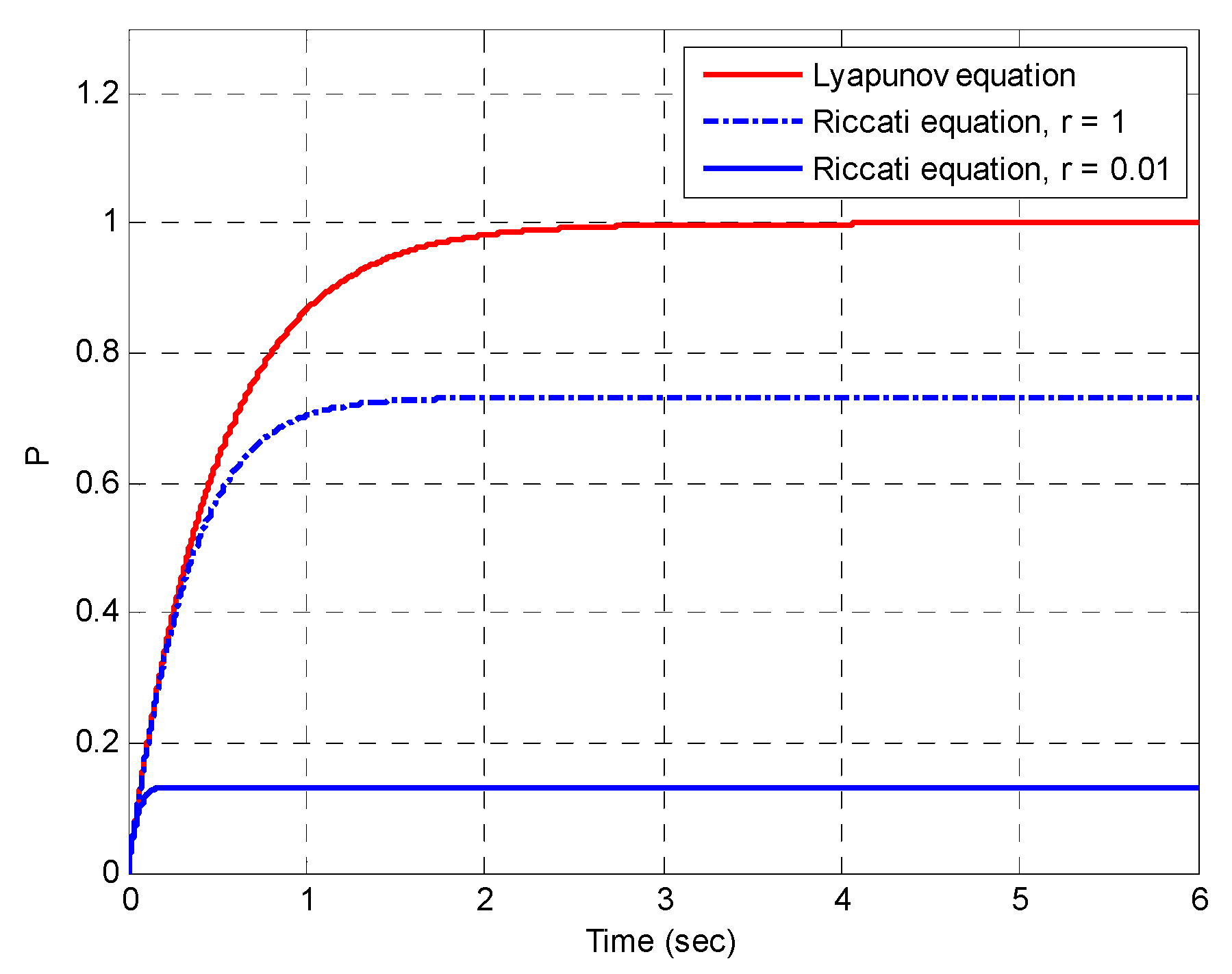
Figure 2 illustrates performance deterioration due to increase in $r$, where $r=1$ and $0.01$ are shown. The result based on Riccati equation with $r\to \infty$ results in the same result as that based on Lyapunov equation. It can be seen from the Kalman gain equation $K=P{H}^T{R}^{-1}$ that when the measurement noise r increases to a very large value, $K$ becomes very small and $P$ approaches 1 in this example. Figure 3 shows the variations of covariance and Kalman gain as r increases. For two selected values of r, the corresponding covariance and Kalman gain are given by: (1) $r=0.01$: $P_{\infty }=0.1318$ and $K_{\infty }=13.1774$; (2) $r=1$: $P_{\infty }=0.7321$ and $K_{\infty }=0.7321$, as indicated by the circle symbols in the figure.

The discrete Kalman filter is performed for performance comparison and consistency check between DKF and CKF. The continuous-time equation can be discretized as the following:

$$x_{k+1}=e^{-\beta \Delta t}{x}_k+u_k, u_k~N(0,Q_k)$$

(37)

where the covariance is the following:

$$Q_k=E[x_k^2]={\displaystyle {\int }_0^{\Delta t}{\displaystyle {\int }_0^{\Delta t}h(\xi )h(\eta )E[u(\xi )u(\eta )]d\xi d\eta }}=\frac{q}{2\beta }(1-e^{-2\beta \Delta t})$$

(38)

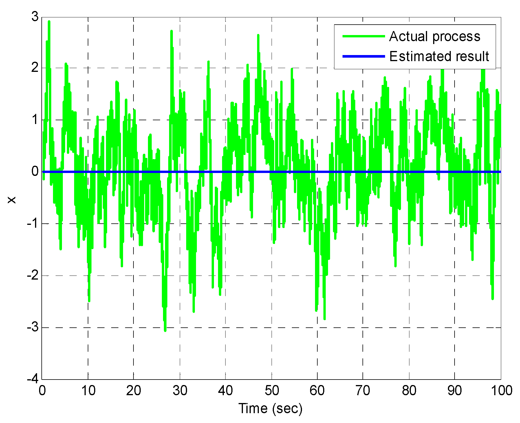
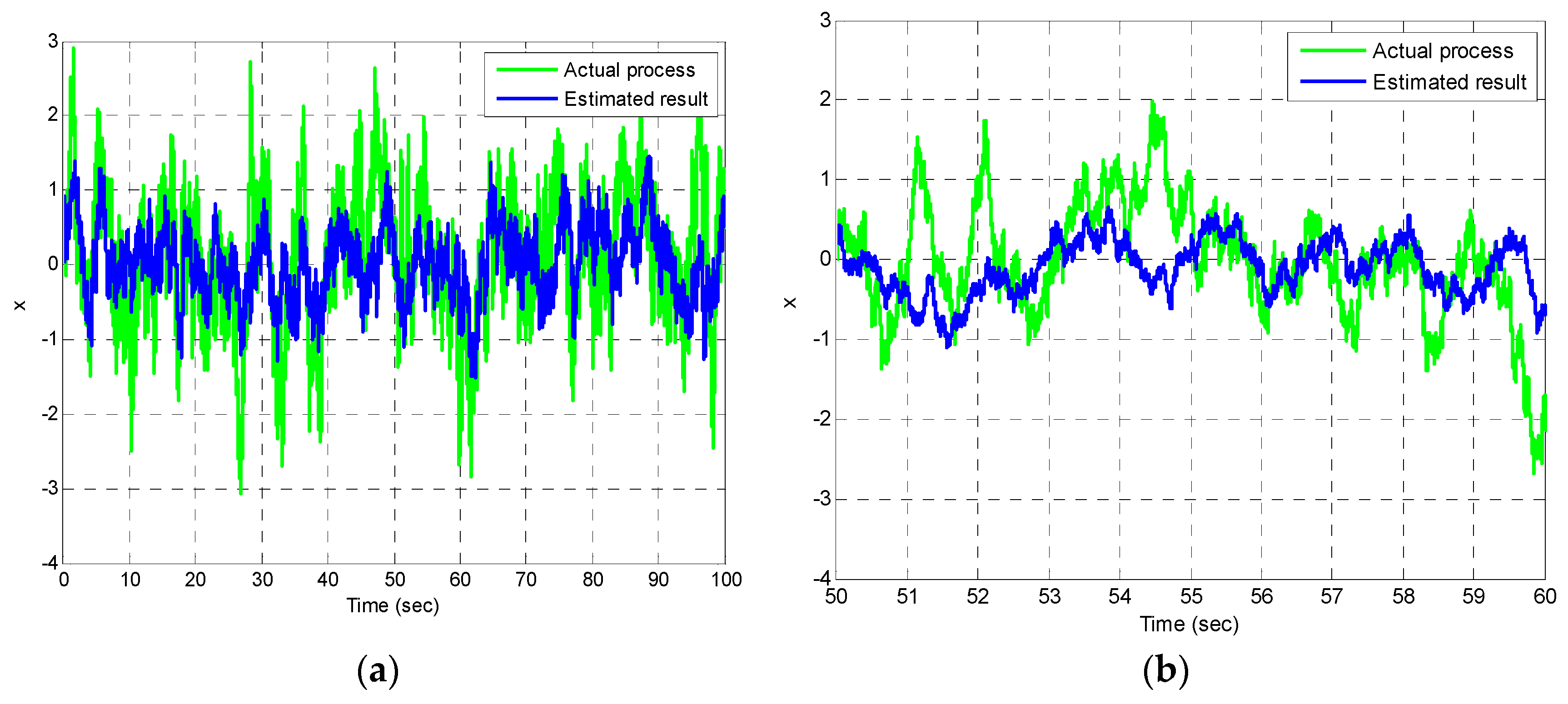
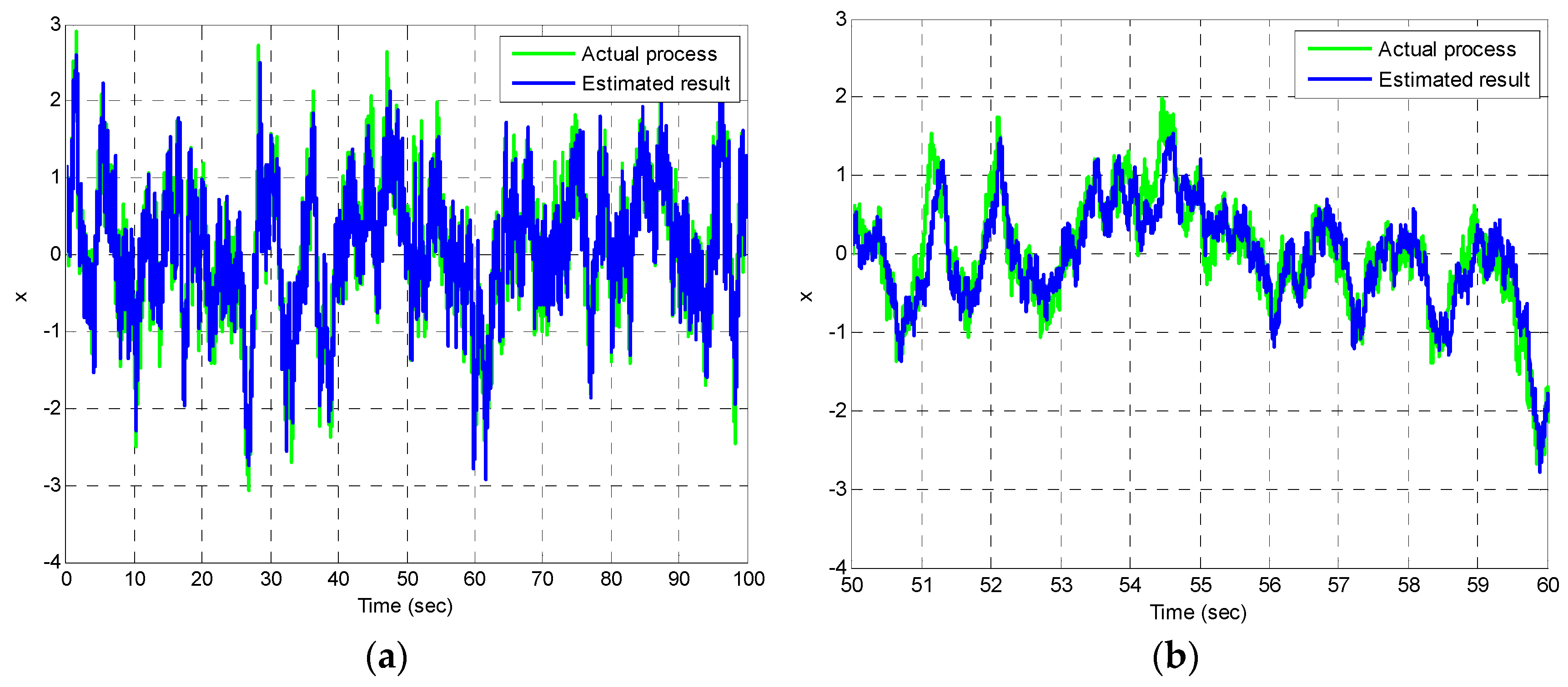
Figure 4, Figure 5 and Figure 6 provide the state estimation results for the first-order Gauss-Markov process with various values of r. The state estimation in the case of a very large measurement noise r ($r\to \infty$) is shown in Figure 4. In this case, the Kalman filter gain approaches 0, and the correction capability on state vector is no longer available, meaning that only time update is implemented. Figure 5 and Figure 6 present the estimation results in the case of larger ($r=1$) and smaller ($r=0.01$) measurement noises, respectively are involved. The plot on the right provides a closer look at the time interval 50–60 s for better observation. To collect the data for calculating the error variance from the estimation results, a recursive loop for evaluating estimation errors is employed based on Figure 7.

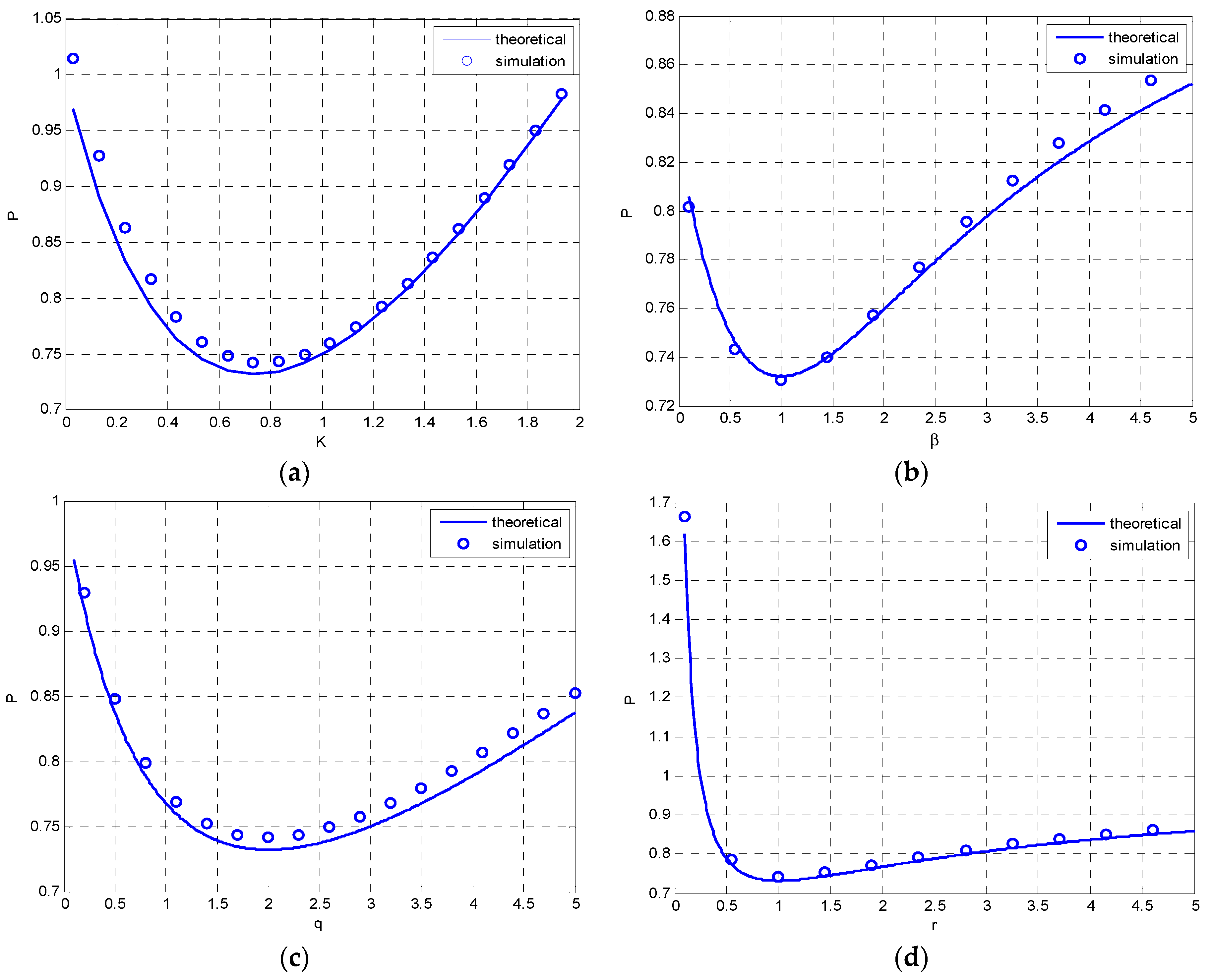
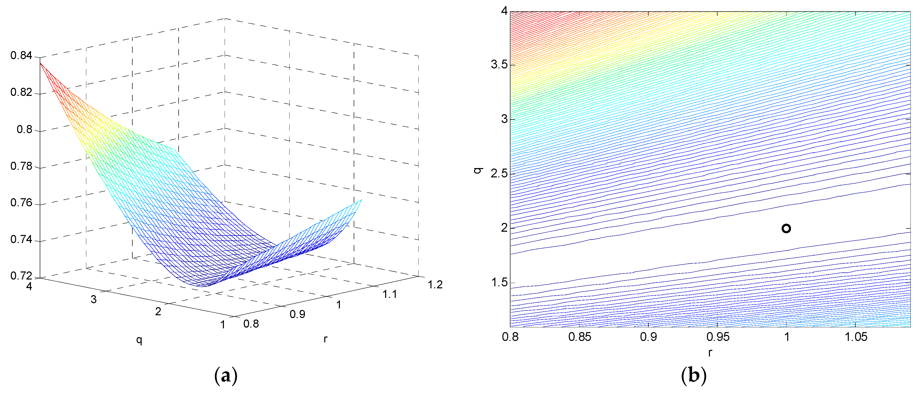
Performance degradation due to deviation of Kalman gain $K$, and three other parameters, including $\beta$, $q$, and $r$, respectively, is examined in Figure 8. In each of the four plots, two sets of results are shown for observation of the effect by deviation of the parameters from the appropriate points and also for consistency check of DKF and CKF results. The solid lines represent the theoretical values while the circles are based on the DKF, respectively. Figure 9 provides a three-dimensional surface and contour of the covariance due to deviation of $q$ and $r$ from the optimal point. In this case $q=2$ and $r=1$, as indicated by a circle symbol on the figure.

4.2. Example 2: An Additional Deterministic Control Input Is Introduced

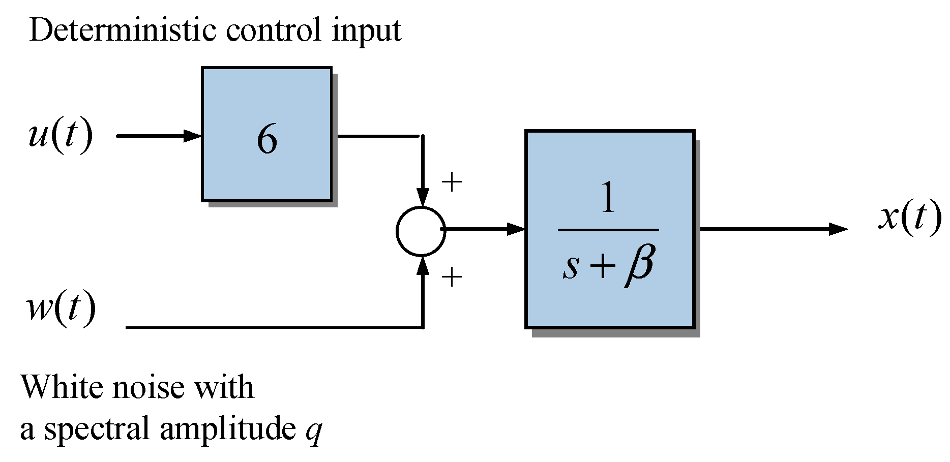
An additional deterministic control input is introduced to the system, shown as in Figure 10. Two extensions of the scalar Gauss-Markov system are presented. Propagation of mean value estimate in continuous-time systems is involved is the discussion. An additional deterministic control input is introduced into the Gauss-Markov process, leading to the system described by the following stochastic differential equation:

$$\frac{dx(t)}{dt}+x(t)=6u(t)+w(t) , w(t)~N(0,q) (\mathrm{i}.\mathrm{e}., \beta =1)$$

(39)

with initial condition $y(0)=0$, where $u(t)$ is the unit step function and $w(t)$ is the unity Gaussian white noise. Since the impulse response is $h(t)=6e^{-\beta t}u(t)$, and therefore the transfer function is given by the following:

$$H(j\omega )=6\cdot \frac{1}{j\omega +\beta }$$

The discrete model discretized from the continuous model can be represented as the following:

$$x_{k+1}=e^{-\beta \Delta t}{x}_k+\Delta t\cdot 6+u_k, u_k~N(0,Q_k)$$

(40)

where the covariance $Q_k$ remains the same as Example 1.

The mean values of the output can be evaluated based on the relation ${\mu }_x(t)={\mu }_f(t)H(0)$:

$${\mu }_x(t)=6\cdot \frac{1}{\beta }=6$$

and the error covariance are thus given by the following:

$$P_{\infty }=-\beta r+\sqrt{{\beta }^2{r}^2+qr}=\sqrt{3}-1\approx 0.7321$$

Figure 11 provides the estimation result in the case of additional deterministic control input. The plot on the right provides a close look at the time interval 0–10 s. The curve in black indicates the response due to the deterministic control input. The results are consistent with the theoretical result shown as in Figure 2 in Example 1.

4.3. Example 3: A Larger Gain Is Applied to the System

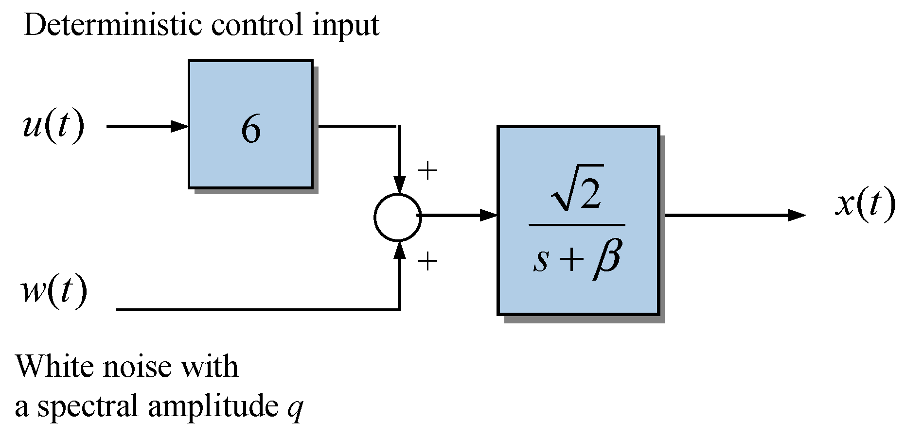
A larger gain is applied to the system, shown as in Figure 12. A larger gain applied to the system leads to the system described by the following stochastic differential equation:

$$\frac{dx(t)}{dt}+x(t)=\sqrt{2}(6u(t)+w(t)) , w(t)~N(0,q)$$

(41)

with initial condition $y(0)=0$, where $u(t)$ is the unit step function and $w(t)$ is the unity Gaussian white noise.

The discrete model from the continuous model can be represented as the following:

$$x_{k+1}=e^{-\beta \Delta t}{x}_k+\Delta t\cdot 6\sqrt{2}+u_k, u_k~N(0,2Q_k)$$

(42)

where the covariance is two times larger than the previous two examples.

The transfer function as follows:

$$H(j\omega )=6\cdot \frac{\sqrt{2}}{j\omega +\beta }$$

Accordingly, the output mean values based on the relation ${\mu }_x(t)={\mu }_f(t)H(0)$ and the error covariance, respectively, are given by the following:

$${\mu }_x(t)=6\frac{\sqrt{2}}{\beta }=6\sqrt{2}\approx 8.485; P_{\infty }=\sqrt{5}-1\approx 1.2361$$

Figure 13 provides the estimation result in the case of a larger gain involved. As a check of consistency, the result based on the DKF $P_k=1.2353$ matches very well with the result based on CKF.

4.4. Example 4: The Integrated Gauss-Markov Process

The integrated Gauss-Markov process shown in Figure 14 is frequently in engineering applications. By defining two state variables, $x_1=x$ and $x_2=\dot{x}$, the corresponding continuous model is as follows:

$$\frac{d}{dt}\left[\begin{array}{c}{x}_1\\ x_2\end{array}\right]=\left[\begin{array}{cc}0& 1\\ 0& -\beta \end{array}\right]\left[\begin{array}{c}{x}_1\\ x_2\end{array}\right]+\left[\begin{array}{c}0\\ 1\end{array}\right]w(t), w(t)~N(0,q)$$

(43)

The mean-square values for this integrated Gauss-Markov process can be shown to be the following:

$$E[x_1^2]=\frac{q}{{\beta }^2}\left[t-\frac{2}{\beta }(1-e^{-\beta t})+\frac{1}{2\beta }(1-e^{-2\beta t})\right]$$

$$E[x_1{x}_2]=\frac{q}{{\beta }^2}\left[(1-e^{-\beta t})-\frac{1}{2}(1-e^{-2\beta t})\right]$$

$$E[x_2^2]=\frac{q}{2\beta }(1-e^{-2\beta t})$$

and as $t\to \infty$, the error covariance matrix is approaching the following:

$$P_{\infty }=\left[\begin{array}{cc}E[x_1^2]& E[x_1{x}_2]\\ E[x_1{x}_2]& E[x_2^2]\end{array}\right]\to \left[\begin{array}{cc}\infty & 1\\ 1& 1\end{array}\right].$$

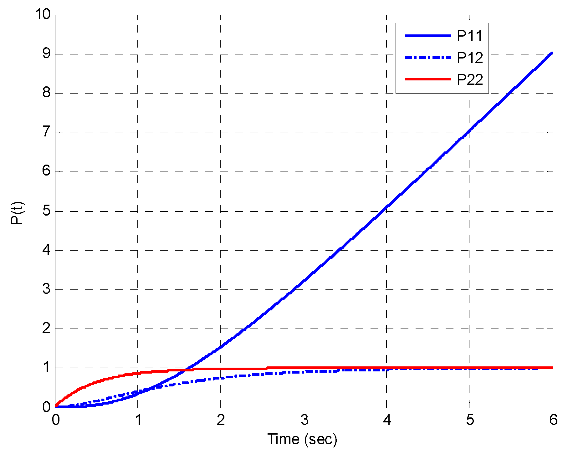
The mean-square value of $x_1$, namely the error covariance $P_{11}=E[x_1^2]$ grows unbounded.

The time history of covariances can be obtained using numerical integration for solving the Riccati equation:

$$\begin{array}{c}{\dot{P}}_{11}=2P_{12}-\frac{1}{r}{P}_{11}^2\\ {\dot{P}}_{12}=P_{22}-\beta P_{12}-\frac{1}{r}{P}_{11}{P}_{12}\\ {\dot{P}}_{22}=q-2\beta P_{22}-\frac{1}{r}{P}_{12}^2\end{array}$$

(44)

Figure 15 shows the propagation of the error covariance when no measurement is available for the integrated Gauss-Markov process, using the Lyapunov equation, which can be regarded as the Riccati equation by setting $r\to \infty$. When the measurement is available, Figure 16 presents the propagation of the error covariance and Kalman gains for the integrated Gauss-Markov process using the Riccati equation of KF. The steady-state error covariance and Kalman gain matrices for the integrated Gauss-Markov process by CKF are the following:

$$P_{\infty }=\left[\begin{array}{cc}0.9566& 0.4576\\ 0.4576& 0.8953\end{array}\right]; K_{\infty }=\left[\begin{array}{c}0.9566\\ 0.4576\end{array}\right].$$

To implement the DKF, the parameters ${\Phi }_k$ and $Q_k$ are found to be the following:

$${\Phi }_k={\left[{\pounds }^{-1}[{(SI-F)}^{-1}]\right]}_{t=\Delta t}=\left[\begin{array}{cc}1& \frac{1}{\beta }(1-e^{-\beta \Delta t})\\ 0& e^{-\beta \Delta t}\end{array}\right]; Q_k=\left[\begin{array}{cc}E[x_1^2]& E[x_1{x}_2]\\ E[x_1{x}_2]& E[x_2^2]\end{array}\right]$$

where

$$F=\left[\begin{array}{cc}0& 1\\ 0& -\beta \end{array}\right]$$

$$E[x_1^2]=\frac{q}{{\beta }^2}\left[\Delta t-\frac{2}{\beta }(1-e^{-\beta \Delta t})+\frac{1}{2\beta }(1-e^{-2\beta \Delta t})\right]$$

$$E[x_1{x}_2]=\frac{q}{{\beta }^2}\left[(1-e^{-\beta \Delta t})-\frac{1}{2}(1-e^{-2\beta \Delta t})\right]$$

$$E[x_2^2]=\frac{q}{2\beta }(1-e^{-2\beta \Delta t})$$

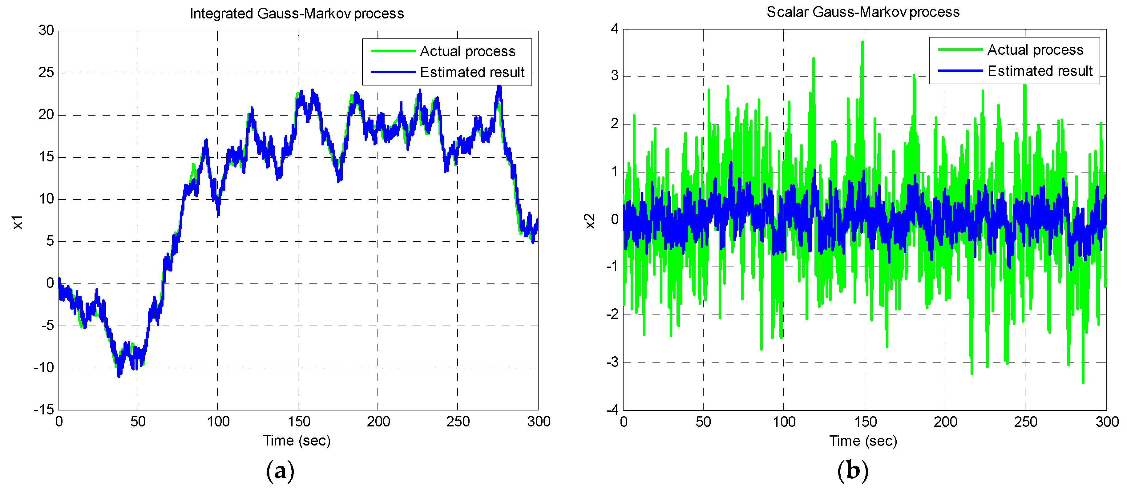
Figure 17 shows the time histories of trajectories for the two states based on the KF compared to the actual process, for the integrated Gauss-Markov process. The results from DKF are given as $P_k=P_{\infty }$, and the following:

$$K_k=\left[\begin{array}{l}0.9562\\ 0.4574\end{array}\right]\cdot {10}^{-3}$$

which is very close to the following result based on the CKF:

$$K_k\approx K_{\infty }\Delta t=0.001\cdot \left[\begin{array}{c}0.9566\\ 0.4576\end{array}\right].$$

The results form the DKF are shown to be consistent with those from CKF very well.

5. Conclusions

This paper can be served to the readers as a supplement note for the Kalman filter for a better understanding of the topic without requiring a deep theoretical understanding of probability and stochastic process, as well as system theory. The illustrative examples are employed to provide further insights into understanding the analysis and design of the Kalman filter both qualitatively and quantitatively, enabling the readers to correctly interpret the theory, practice the algorithms, and design the computer codes. This article provides a good explanation of the Kalman filter with illustrative examples so the reader can have a grasp of some of the basic principles. A detailed description is accompanied by several examples offered for clear illustration to provide readers a better understanding of this topic.

The supporting examples employed in this work include the scalar Gauss-Markov process, followed by two extensions of the process, including an additional deterministic control input introduced, a larger gain applied, and finally an integrated Gauss-Markov process. The main issues covered are the connection between the two types of Kalman filters based on DKF and CKF and the verification of results by theoretical and numerical approaches. A consistence check of results for DKF and CKF, including mean value, mean-square value, Kalman gain, and theoretical covariance is provided. Performance degradation caused by the deviation from the optimal point due to parameter uncertainties as presented were also involved are unbounded errors caused by unavailable measurement and bounded errors due to available measurement updates. Besides, the influence on the estimation results when an additional control input is introduced as well as a larger gain applied to the dynamical system selected for illustration.

This presented material is especially helpful for those with less experience or background on the optimal estimation theory to build up a solid foundation for further study on the theory and applications of the topic.

References

1. Kalman, R.E. A New Approach to Linear Filtering and Prediction Problems. Trans. ASME—J. Basic Eng. 1960, 82, 35–45. [Google Scholar] [CrossRef] [Green Version]
2. Brown, R.G.; Hwang, P.Y.C. Introduction to Random Signals and Applied Kalman Filtering; John Wiley & Sons: New York, NY, USA, 1997. [Google Scholar]
3. Gelb, A. Applied Optimal Estimation; M.I.T. Press: Cambridge, MA, USA, 1974. [Google Scholar]
4. Grewal, M.S.; Andrews, A.P. Kalman Filtering, Theory and Practice Using MATLAB, 2nd ed.; John Wiley & Sons, Inc.: New York, NY, USA, 2001. [Google Scholar]
5. Lewis, F.L. Optimal Estimation; John Wiley & Sons, Inc.: New York, NY, USA, 1986. [Google Scholar]
6. Lewis, F.L.; Xie, L.; Popa, D. Optimal and Robust Estimation, with an Introduction to Stochastic Control Theory, 2nd ed.; CRC Press: Boca Raton, FL, USA, 2008. [Google Scholar]
7. Maybeck, S.P. Stochastic Models, Estimation, and Control; Academic Press: New York, NY, USA, 1978; Volume 1. [Google Scholar]
8. Zhu, J.; Chang, X.; Zhang, X.; Su, Y.; Long, X. A Novel Method for the Reconstruction of Road Profiles from Measured Vehicle Responses Based on the Kalman Filter Method. CMES-Comput. Model. Eng. Sci. 2022, 130, 1719–1735. [Google Scholar] [CrossRef]
9. Zhao, S.; Jiang, C.; Zhang, Z.; Long, X. Robust Remaining Useful Life Estimation Based on an Improved Unscented Kalman Filtering Method. CMES-Comput. Model. Eng. Sci. 2020, 123, 1151–1173. [Google Scholar] [CrossRef]
10. Xu, B.; Bai, L.; Chen, K.; Tian, L. A resource saving FPGA implementation approach to fractional Kalman filter. IET Control Theory Appl. 2022, 16, 1352–1363. [Google Scholar] [CrossRef]
11. Won, J.H.; Dötterböck, D.; Eissfeller, B. Performance comparison of different forms of Kalman filter approaches for a vector-based GNSS signal tracking loop. Navigation 2010, 57, 185–199. [Google Scholar] [CrossRef]
12. Zhang, J.H.; Li, P.; Jin, C.C.; Zhang, W.A.; Liu, S. A novel adaptive Kalman filtering approach to human motion tracking with magnetic-inertial sensors. IEEE Trans. Ind. Electron. 2019, 67, 8659–8669. [Google Scholar] [CrossRef]
13. Wang, W.; Liu, Z.Y.; Xie, R.R. Quadratic extended Kalman filter approach for GPS/INS integration. Aerosp. Sci. Technol. 2006, 10, 709–713. [Google Scholar] [CrossRef]
14. Wiltshire, R.A.; Ledwich, G.; O’Shea, P. A Kalman filtering approach to rapidly detecting modal changes in power systems. IEEE Trans. Power Syst. 2007, 22, 1698–1706. [Google Scholar] [CrossRef] [Green Version]
15. Jwo, D.J. Remarks on the Kalman filtering simulation and verification. Appl. Math. Comput. 2007, 186, 159–174. [Google Scholar] [CrossRef]
16. Kwan, C.M.; Lewis, F.L. A note on Kalman filtering. IEEE Trans. Educ. 1999, 42, 225–228. [Google Scholar] [CrossRef]
17. Welch, G.; Bishop, G. An Introduction to the Kalman Filter; Technical Report TR 95-041; University of North Carolina, Department of Computer Science: Chapel Hill, NC, USA, 2006; Available online: https://www.cs.unc.edu/~welch/media/pdf/kalman_intro.pdf (accessed on 30 July 2010).
18. Rhudy, M.B.; Salguero, R.A.; Holappa, K. A Kalman filtering tutorial for undergraduate students. Int. J. Comput. Sci. Eng. Surv. 2017, 8, 1–18. [Google Scholar] [CrossRef]
19. Love, A.; Aburdene, M.; Zarrouk, R.W. Teaching Kalman filters to undergraduate students. In Proceedings of the 2001 American Society for Engineering Education Annual Conference & Exposition, Albuquerque, NM, USA, 24–27 June 2001; pp. 6.950.1–6.950.19. [Google Scholar]
20. Song, T.L.; Ahn, J.Y.; Park, C. Suboptimal filter design with pseudomeasurements for target tracking. IEEE Trans. Aerosp. Electron. Syst. 1988, 24, 28–39. [Google Scholar] [CrossRef]
21. Sun, S. Multi-sensor weighted fusion suboptimal filtering for systems with multiple time delayed measurements. In Proceedings of the 2006 6th World Congress on Intelligent Control and Automation, Dalian, China, 21–23 June 2006; Volume 1, pp. 1617–1620. [Google Scholar]
22. Fronckova, K.; Prazak, P. Possibilities of Using Kalman Filters in Indoor Localization. Mathematics 2020, 8, 1564. [Google Scholar] [CrossRef]
23. Correa-Caicedo, P.J.; Rostro-González, H.; Rodriguez-Licea, M.A.; Gutiérrez-Frías, Ó.O.; Herrera-Ramírez, C.A.; Méndez-Gurrola, I.I.; Cano-Lara, M.; Barranco-Gutiérrez, A.I. GPS Data Correction Based on Fuzzy Logic for Tracking Land Vehicles. Mathematics 2021, 9, 2818. [Google Scholar] [CrossRef]
Figure 1. Block diagram of Example 1: the scalar Gauss-Markov process.
Mathematics 11 00521 g001
Figure 2. Performance deterioration due to increase in r , where r = 1 versus 0.01 are provided. The result based on Riccati equation with r results in that based on Lyapunov equation.
Mathematics 11 00521 g002
Figure 3. Variations of (a) covariance and (b) Kalman gain as r increases.
Mathematics 11 00521 g003
Figure 4. State estimation for the first-order Gauss-Markov process in the case of very large measurement noise r ( r ).
Mathematics 11 00521 g004
Figure 5. State estimation for the first–order Gauss–Markov process in the case of larger measurement noise ( r = 1 ) involved: (a) state estimation; (b) a closer look.
Mathematics 11 00521 g005
Figure 6. State estimation for the first–order Gauss–Markov process in the case of smaller measurement noise ( r = 0.01 ) involved: (a) state estimation; (b) a closer look.
Mathematics 11 00521 g006
Figure 7. Recursive loop for evaluating estimation errors.
Mathematics 11 00521 g007
Figure 8. Performance degradation due to deviation of (a) K (b) β (c) q (d) r , respectively.
Mathematics 11 00521 g008
Figure 9. Three–dimensional surface and contour of the covariance due to deviation of q and r from the optimal point (in this case q = 2 and r = 1 , as indicated by a circle symbol on the figure) (a) surface plot; (b) contour plot.
Mathematics 11 00521 g009
Figure 10. Block diagram of Example 2: the scalar Gauss-Markov process with a deterministic control input.
Mathematics 11 00521 g010
Figure 11. Estimation results for Example 2. The plot on the right provides a closer look at the time interval 0–10 s: (a) estimation results; (b) a closer look.
Mathematics 11 00521 g011
Figure 12. Block diagram of Example 3: the scalar Gauss–Markov process with a larger gain.
Mathematics 11 00521 g012
Figure 13. Estimation results for Example 3. The plot on the right provides a closer look at the time interval 0–10 s: (a) estimation results; (b) a closer look.
Mathematics 11 00521 g013
Figure 14. Block diagram of Example 4: the Integrated Gauss-Markov process.
Mathematics 11 00521 g014
Figure 15. Propagation of the error covariance for the integrated Gauss–Markov process when no measurement is available using the Lyapunov equation.
Mathematics 11 00521 g015
Figure 16. Propagation of the error covariance and Kalman gains for the integrated Gauss–Markov process using the Riccati equation of KF: (a) error covariance; (b) Kalman gains.
Mathematics 11 00521 g016
Figure 17. Propagation of the two states using KF for the integrated Gauss–Markov process KF: (a) first state; (b) second state.
Mathematics 11 00521 g017