
Scale Mixture of Maxwell-Boltzmann Distribution

 ,
,  ,
,  ,
,  and
and 
Abstract
:1. Introduction
2. Definition and Properties
2.1. Lifetime Analysis
2.2. Moments
2.3. Order Statistics
2.4. Entropy
3. Inference
3.1. Moments Estimators
3.2. Maximum Likelihood Estimator
3.3. EM-Algorithm
- 1 .
- , with pdf given in (1).
- 2 .
- .
- Step-E: For compute
- Step-M: Update the parameters as
3.4. Fisher’s Information Matrix
4. Simulation Study
- 1.
- Generate (chi squared with 3 degrees of freedom),
- 2.
- Compute ,
- 3.
- Generate ,
- 4.
- Compute
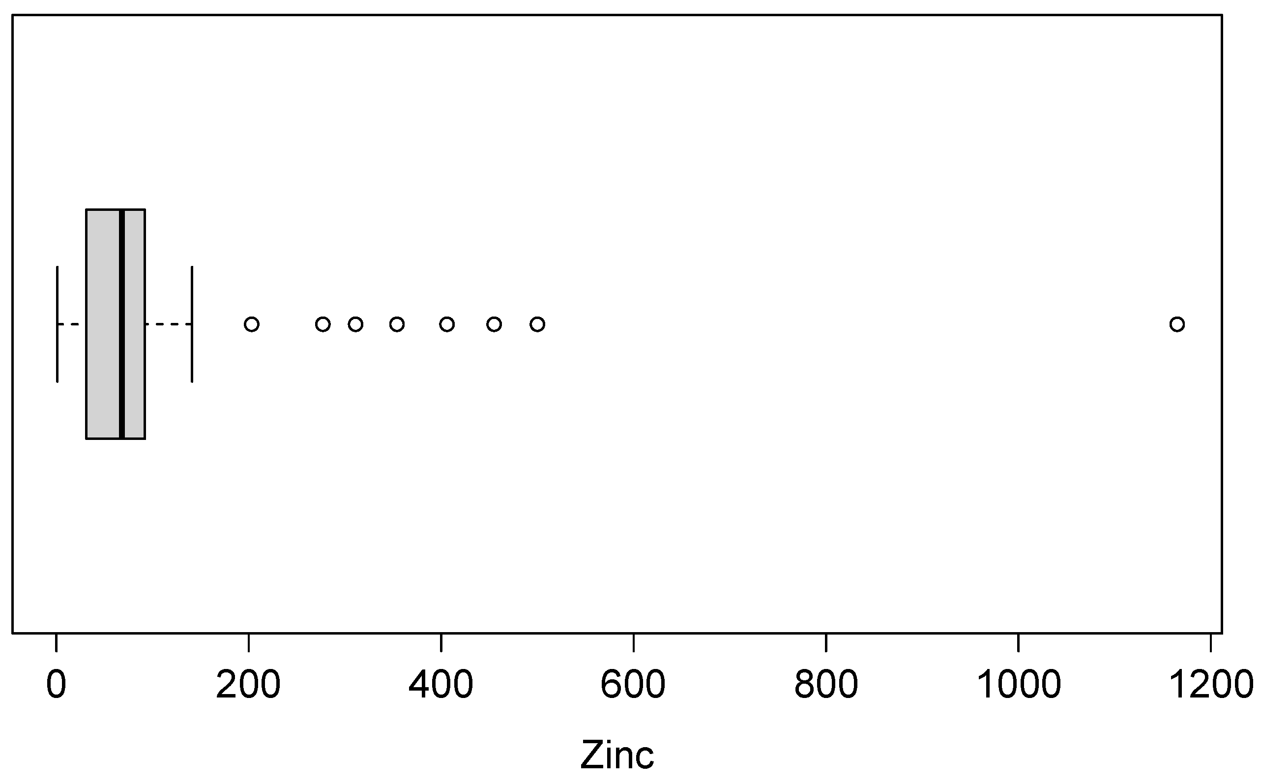
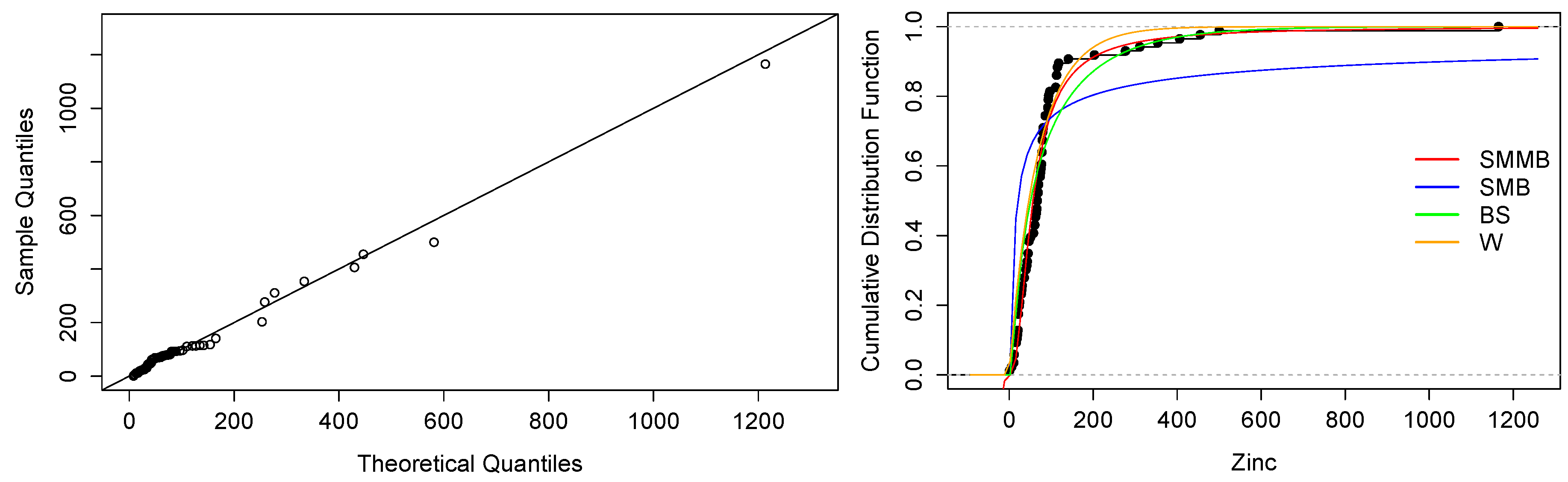
5. Application
6. Conclusions
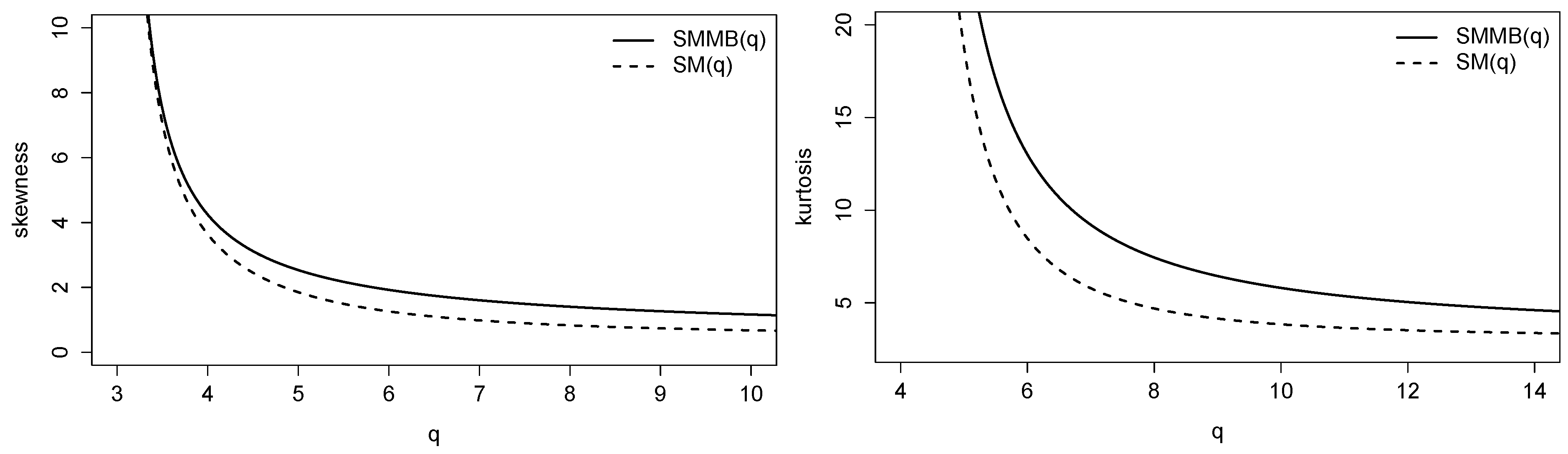
- SMMB distribution has a more flexible kurtosis coefficient than the SMB distribution, as is clearly shown in Figure 4 (Right panel)
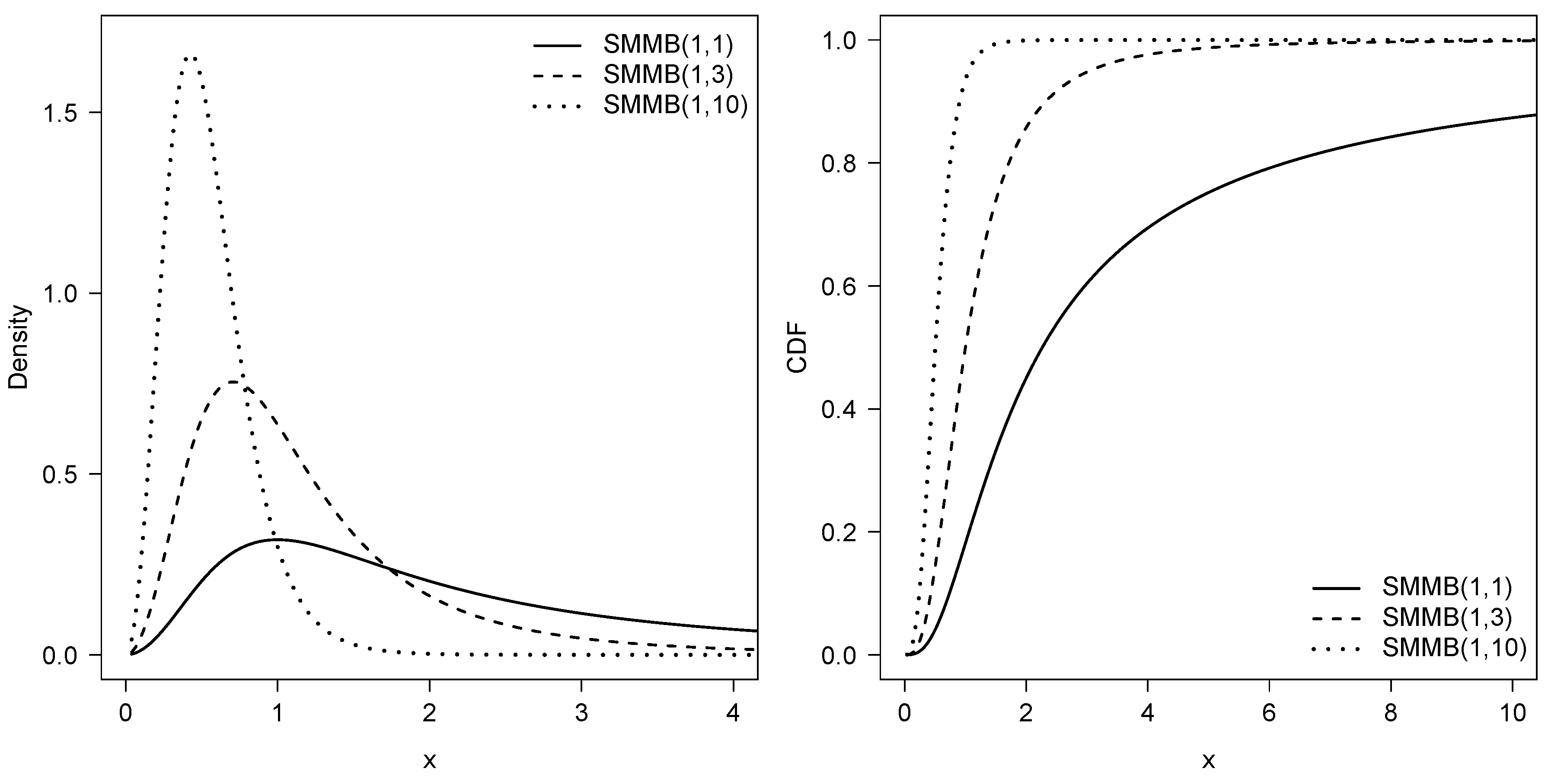
- Closed expressions are given for its main characteristics: pdf, cdf, moments and coefficients of skewness and kurtosis.
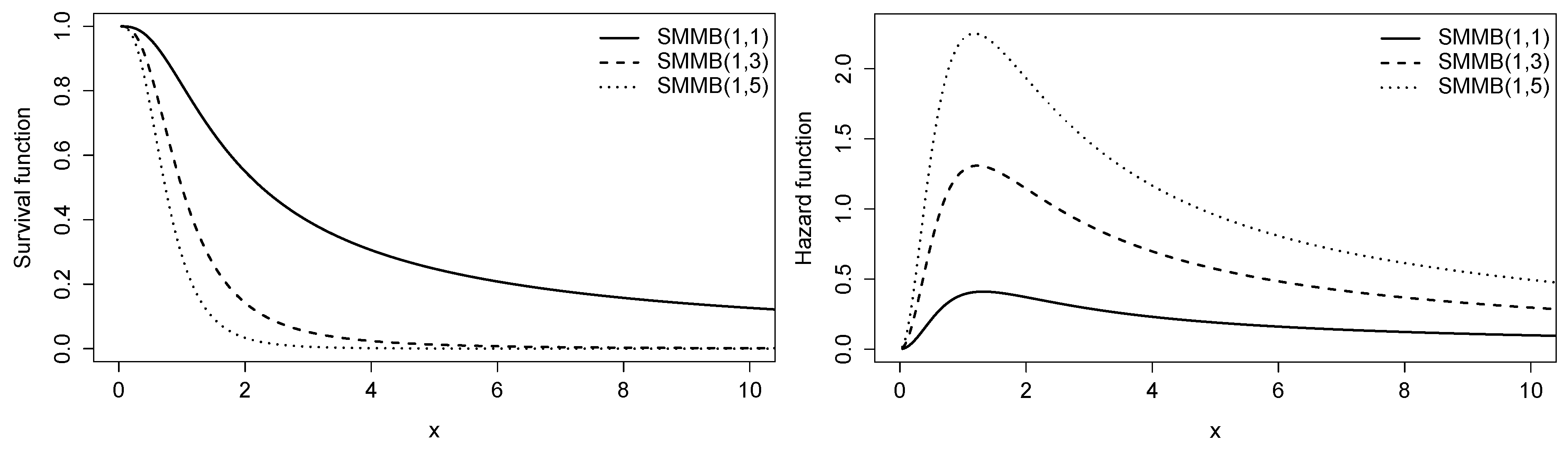
- We discuss the hazard and survival functions, which are in terms of the hypergeometric function and the order statistics of the SMMB model.
- Employing the scale mixture representation, the EM algorithm was implemented to calculate the ML estimators.
- The results of a simulation study indicate that, with a reasonable sample size, an acceptable bias is obtained.
- An illustration with real data shows that the SMMB model achieves a better fit in terms of the AIC and BIC criteria.
Author Contributions
Funding
Institutional Review Board Statement
Informed Consent Statement
Data Availability Statement
Conflicts of Interest
Appendix A
References
- Maxwell, J. On the dynamical theory of gases. Philos. Trans. R. Soc. Lond. 1867, 35, 185–217. [Google Scholar]
- Tyagi, R.K.; Bhattacharya, S.K. Bayes estimation of the Maxwell’s velocity distribution function. J. Stat. Comput. Simul. 1989, 29, 563–567. [Google Scholar]
- Bekker, A.; Roux, J. Reliability characteristics of the Maxwell distribution: A bayes estimation study. Commun. Stat. Theory Methods 2005, 34, 2169–2178. [Google Scholar] [CrossRef]
- Sharma, V.K.; Bakouch, H.S.; Suthar, K. An extended Maxwell distribution: Properties and applications. Commun. Stat. Simul. Comput. 2017, 46, 6982–7007. [Google Scholar] [CrossRef]
- Vivekanand, H.K.; Kumar, K. Estimation in Maxwell distribution with randomly censored data. J. Stat. Comput. Simul. 2015, 85, 4264–4274. [Google Scholar] [CrossRef]
- Iriarte, Y.A.; Astorga, J.M.; Gómez, H.W. Gamma-Maxwell distribution. Commun. Stat. Theory Methods 2017, 46, 4264–4274. [Google Scholar] [CrossRef]
- Dey, S.; Dey, T.; Ali, S.; Mulekar, M.S. Two-parameter Maxwell distribution: Properties and different methods of estimation. J. Stat. Theory. Pract. 2016, 10, 394–403. [Google Scholar] [CrossRef]
- Sharma, V.K.; Dey, S.; Singh, S.K.; Manzoor, U. On length and area-biased Maxwell distributions. Commun. Stat. Simul. Comput. 2017, 47, 1506–1528. [Google Scholar] [CrossRef]
- Segovia, F.; Gómez, Y.M.; Gallardo, D.I. Exponentiated power Maxwell distribution with quantile regression and applications. SORT 2021, 45, 181–200. [Google Scholar]
- Shakil, M.; Golam, B.; Chang, K. Distributions of the product and ratio of Maxwell and Rayleigh random variables. Stat. Pap. 2008, 49, 729–747. [Google Scholar] [CrossRef]
- Acitas, S.; Arslan, T.; Senoglu, B. Slash Maxwell distribution: Definition, modified maximum likelihood estimation and applications. Gazi Univ. J. Sci. 2020, 33, 249–263. [Google Scholar] [CrossRef]
- Reyes, J.; Barranco-Chamorro, I.; Gómez, H.W. Generalized modified slash distribution with applications. Commun. Stat.-Theory Methods 2020, 49, 2025–2048. [Google Scholar] [CrossRef]
- Astorga, J.M.; Reyes, J.; Santoro, K.I.; Venegas, O.; Gómez, H.W. A Reliability Model Based on the Incomplete Generalized Integro-Exponential Function. Mathematics 2020, 8, 1537. [Google Scholar] [CrossRef]
- Stacy, E.W. A generalization of the gamma distribution. An. Math. Stat. 1962, 33, 1187–1192. [Google Scholar] [CrossRef]
- Abramowitz, M.; Stegun, I.E. Handbook of Mathematical Functions with Formulas, Graphs, and Mathematical Tables, 9th ed.; National Bureau of Standars: Washington, DC, USA, 1970. [Google Scholar]
- Singh, P. Hypergeometric Functions on Cumulative Distribution Function. Asian Res. J. Math. 2019, 13, 1–11. [Google Scholar] [CrossRef] [Green Version]
- Glaser, R.E. Bathtub and Related Failure Rate Characterizations. J. Am. Stat. Assoc. 1980, 75, 667–672. [Google Scholar] [CrossRef]
- Weisstein, E.W. “Hypergeometric Function”. From MathWorld—A Wolfram Web Resource. Available online: https://mathworld.wolfram.com/HypergeometicFunction.html (accessed on 2 January 2023).
- R Core Team. R: A Language and Environment for Statistical Computing; R Foundation for Statistical Computing: Vienna, Austria, 2022; Available online: https://www.R-project.org/ (accessed on 2 January 2023).
- Dempster, A.P.; Laird, N.M.; Rubim, D.B. Maximum likelihood from incomplete data via the EM algorithm (with discussion). J. R. Stat. Soc. Ser. B 1977, 39, 1–38. [Google Scholar]
- Akaike, H. A new look at the statistical model identification. IEEE Trans. Autom. Control. 1974, 19, 716–723. [Google Scholar] [CrossRef]
- Schwarz, G. Estimating the dimension of a model. Ann. Stat. 1978, 6, 461–464. [Google Scholar] [CrossRef]
- Reyes, J.; Rojas, M.A.; Venegas, O.; Gómez, H.W. Nakagami Distribution with Heavy Tails and Applications to Mining Engineering Data. J. Stat. Theory Pract. 2020, 14, 55. [Google Scholar] [CrossRef]
- Morán-Vásquez, R.A.; Mazo-Lopera, M.A.; Ferrari, S.L.P. Quantile modeling through multivariate log-normal/independent linear regression models with application to newborn data. Biom. J. 2021, 63, 1290–1308. [Google Scholar] [CrossRef] [PubMed]
- Lange, K.; Sinsheimer, J.S. Normal/Independent Distributions and Their Applications in Robust Regression. J. Comput. Graph. Stat. 1993, 2, 175–198. [Google Scholar]


| q | q | ||
| 1 | 5 | ||
| 2 | 6 | ||
| 3 | 7 | ||
| 4 | 8 |
| True Value | ||||||||||||||
|---|---|---|---|---|---|---|---|---|---|---|---|---|---|---|
| Estim. | Bias | SE | RMSE | CP | Bias | SE | RMSE | CP | Bias | SE | RMSE | CP | ||
| 3 | 1 | 0.113 | 1.294 | 1.334 | 90.1 | 0.074 | 0.897 | 0.925 | 92.1 | 0.027 | 0.623 | 0.661 | 92.2 | |
| 0.057 | 0.216 | 0.232 | 96.5 | 0.024 | 0.145 | 0.153 | 95.0 | 0.016 | 0.102 | 0.111 | 94.1 | |||
| 2 | 0.065 | 1.290 | 1.335 | 90.1 | 0.039 | 0.896 | 0.921 | 92.5 | 0.019 | 0.628 | 0.665 | 91.8 | ||
| 0.211 | 0.613 | 0.709 | 95.9 | 0.090 | 0.388 | 0.426 | 95.5 | 0.052 | 0.265 | 0.296 | 94.9 | |||
| 3 | 0.040 | 1.396 | 1.444 | 89.6 | 0.015 | 0.966 | 0.996 | 92.1 | 0.009 | 0.679 | 0.709 | 92.0 | ||
| 0.524 | 1.329 | 1.625 | 95.7 | 0.226 | 0.758 | 0.892 | 95.1 | 0.115 | 0.495 | 0.558 | 95.2 | |||
| 5 | 1 | 0.188 | 2.155 | 2.222 | 90.1 | 0.122 | 1.495 | 1.541 | 92.1 | 0.044 | 1.038 | 1.102 | 92.2 | |
| 0.057 | 0.216 | 0.232 | 96.5 | 0.024 | 0.145 | 0.153 | 95.1 | 0.016 | 0.102 | 0.111 | 94.1 | |||
| 2 | 0.106 | 2.149 | 2.224 | 90.1 | 0.064 | 1.493 | 1.534 | 92.5 | 0.030 | 1.046 | 1.108 | 91.8 | ||
| 0.211 | 0.613 | 0.709 | 95.9 | 0.091 | 0.388 | 0.426 | 95.5 | 0.053 | 0.265 | 0.296 | 94.9 | |||
| 3 | 0.061 | 2.324 | 2.410 | 89.5 | 0.024 | 1.610 | 1.659 | 92.1 | 0.014 | 1.132 | 1.182 | 92.0 | ||
| 0.567 | 1.478 | 2.120 | 95.7 | 0.227 | 0.758 | 0.892 | 95.1 | 0.116 | 0.495 | 0.558 | 95.2 | |||
| 7 | 1 | 0.262 | 3.017 | 3.111 | 90.1 | 0.169 | 2.093 | 2.157 | 92.1 | 0.061 | 1.453 | 1.542 | 92.2 | |
| 0.057 | 0.216 | 0.232 | 96.5 | 0.024 | 0.145 | 0.153 | 95.1 | 0.016 | 0.102 | 0.111 | 94.1 | |||
| 2 | 0.148 | 3.008 | 3.113 | 90.1 | 0.088 | 2.090 | 2.148 | 92.5 | 0.041 | 1.464 | 1.550 | 91.8 | ||
| 0.211 | 0.613 | 0.709 | 95.9 | 0.091 | 0.388 | 0.426 | 95.5 | 0.053 | 0.265 | 0.296 | 94.9 | |||
| 3 | 0.078 | 3.251 | 3.378 | 89.4 | 0.033 | 2.254 | 2.322 | 92.1 | 0.019 | 1.585 | 1.655 | 92.0 | ||
| 0.610 | 1.566 | 2.519 | 95.7 | 0.227 | 0.758 | 0.892 | 95.1 | 0.116 | 0.495 | 0.559 | 95.2 | |||
| n | s | |||
|---|---|---|---|---|
| 86 | 96.721 | 148.434 | 5.088 | 32.342 |
| Parameters | BS | W | SMB | SMMB |
|---|---|---|---|---|
| 1.3038 (0.0995) | 0.0125 (0.0047) | 3.4666 (0.1226) | - | |
| 50.8841 (5.8694) | 0.9632 (0.0701) | - | 0.0007 (0.0002) | |
| q | - | - | 0.4077 (0.1827) | 1.6506 (0.3079) |
| log-likelihood | −484.7785 | −479.0418 | −471.7718 | −469.5580 |
| AIC | 973.557 | 962.084 | 947.544 | 943.1161 |
| BIC | 978.466 | 966.992 | 952.452 | 948.0248 |
Disclaimer/Publisher’s Note: The statements, opinions and data contained in all publications are solely those of the individual author(s) and contributor(s) and not of MDPI and/or the editor(s). MDPI and/or the editor(s) disclaim responsibility for any injury to people or property resulting from any ideas, methods, instructions or products referred to in the content. |
© 2023 by the authors. Licensee MDPI, Basel, Switzerland. This article is an open access article distributed under the terms and conditions of the Creative Commons Attribution (CC BY) license (https://creativecommons.org/licenses/by/4.0/).
Share and Cite
Castillo, J.S.; Gaete, K.P.; Muñoz, H.A.; Gallardo, D.I.; Bourguignon, M.; Venegas, O.; Gómez, H.W. Scale Mixture of Maxwell-Boltzmann Distribution. Mathematics 2023, 11, 529. https://doi.org/10.3390/math11030529
Castillo JS, Gaete KP, Muñoz HA, Gallardo DI, Bourguignon M, Venegas O, Gómez HW. Scale Mixture of Maxwell-Boltzmann Distribution. Mathematics. 2023; 11(3):529. https://doi.org/10.3390/math11030529
Chicago/Turabian StyleCastillo, Jaime S., Katherine P. Gaete, Héctor A. Muñoz, Diego I. Gallardo, Marcelo Bourguignon, Osvaldo Venegas, and Héctor W. Gómez. 2023. "Scale Mixture of Maxwell-Boltzmann Distribution" Mathematics 11, no. 3: 529. https://doi.org/10.3390/math11030529
APA StyleCastillo, J. S., Gaete, K. P., Muñoz, H. A., Gallardo, D. I., Bourguignon, M., Venegas, O., & Gómez, H. W. (2023). Scale Mixture of Maxwell-Boltzmann Distribution. Mathematics, 11(3), 529. https://doi.org/10.3390/math11030529