Hotelling T² Control Chart for Detecting Changes in Mortality Models Based on Machine-Learning Decision Tree

Abstract

Mortality modelling is a practical method for the government and various fields to obtain a picture of mortality up to a specific age for a particular year. However, some information on the phenomenon may remain in the residual vector and be unrevealed from the models. We handle this issue by employing a multivariate control chart to discover substantial cohort changes in mortality behavior that the models still need to address. The Hotelling T² control chart is applied to the externally studentized deviance model, which is already optimized using a machine-learning decision tree. This study shows a mortality model with the lowest MSE, MAPE, and deviance, by accomplishing simulations in various countries. In addition, the model that is more sensitive in detecting signals on the control chart is singled out so that we can perform a decomposition to determine the attributes of death in the specific outlying age group in a particular year. The case study in the decomposition uses data from the country Saudi Arabia. The overall results demonstrate that our method of processing and producing mortality models with machine learning can be a solution for developing countries or countries with limited mortality data to produce accurate predictions through monitoring control charts.

1. Introduction

Demography is a science that studies the number, structure, and changes in the population of an area, where changes in the population structure are influenced by three components, namely birth, death, and migration [1]. Based on this definition, mortality or death is one of the components that can affect changes in population structure.

The mortality rate measures the number of deaths in a population. Many fields such as actuarial science, health, economics, and the government use mortality rates. In government, the mortality rate can be used as an evaluation material for population policy programs and population projections, which will later be used to design the country’s development. In the economic field, when the rate of a country’s mortality is high, its economic needs will reduce. In the health sector, the mortality rate determines the probability of a person surviving a certain period, both micro and macro. In the actuarial field, the mortality rate is used to generate the probability of survival and death and with this, one can determine the premium amount for some life insurance contracts [2].

Attempts to determine models that accurately represent mortality rates have a long history. The authors of [3] highlighted that some of the earlier, well-known research recorded in history has been pioneered by [4,5,6]. Some of these models continue to develop because of the increasing importance of precise and accurate mortality predictions. The dynamics of change in public health conditions, life expectancy, survival probabilities, and the emergence of various outbreaks have also contributed to the adjustment of the mortality model [7]. Three popular existing mortality models are Lee–Carter (LC), Renshaw–Haberman (RH), and Cairns–Blake–Dowd (CBD). These mortality models explain the mortality rate of a population with specific characteristics by fitting it to the mortality data of the population.

However, some information on the phenomenon may remain in the residual vector and be unrevealed by the models. To study in more detail the existence of a death signal or data that have a pattern outside the data group, it is exactly here that the control chart plays a crucial part: trying to uncover some other important changes in mortality behavior that the models have not already addressed. However, there are currently a very small number of articles that discuss the monitoring of changes in mortality modelling using control charts. To the best of our knowledge, the only one is [8], who investigated and studied the use of multivariate control chart in mortality modelling, namely using the LC model. Although the result has been well explained, the models in the paper are approximate and do not meet one of the primary LC model constraints. The use of the Quasi-Poisson setting is one indication of this, which needs further discussion. Meanwhile, other papers utilize control charts for micro mortality data only. Research by [9] uses the EWMA chart on infant mortality, which monitors the residual deviance to see substantial errors, considered as outliers. On the other hand, Ref. [10] examined mortality data in the intensive care unit to be an early warning for the hospital in its services, as seen by in-hospital death cases. The fundamental reason for the lack of mortality studies is the scarcity of mortality data in many nations [11]. It is critical to conduct mortality modelling to project data that can be used by the government, the business sector, and other industries.

To address the above issues, our paper uses the Poisson setting in the LC mortality model to rectify Díaz-Rojo’s LC model, whose parameter model is an approximation. Furthermore, we go beyond modelling mortality in several countries with three models and optimize the model using machine learning. Combining these mortality models with machine learning algorithms might produce better results, because machine learning algorithms can detect hidden patterns in a dataset and hidden correlations between variables in the models [12]. Finally, our paper proposes a multivariate control chart, the Hotelling T², to monitor the three models, developed for both male and female populations. The purpose of using this control chart is to identify situations of substantial change in the mortality trend, and to study the exact outlying mortality age group.

The rest of paper is organized as follows: Section 2 introduces the mortality modelling, discusses the machine learning technique, and explains the Hotelling T² control chart as the multivariate control chart in monitoring the residuals of the models. Implementation details and simulation findings are reported in Section 3. In Section 4, we illustrate the best model from the previous comparison and apply the model to several countries, including Saudi Arabia. After the model was built, the externally studentized deviation was monitored using a Hotelling T² control chart, and then decomposed for more in-depth analysis in specific age groups.

2. Materials and Methods

2.1. Mortality Modelling

The mortality rate measures a population’s mortality for a specific place, time, age, and condition. The mortality rate in a population can be calculated using the equation:

$$m_{x,t}=\frac{d_{x,t}}{l_{x,t}}\times {10}^n$$

(1)

where $m_{x,t}$ is the mortality rate of age group x in period t, $d_{x,t}$ is the number of deaths of people of age group x in the period t, $l_{x,t}$ is the total population of age group x in period t, and n is the value determined by the researcher to control the desired and reported decimal places.

For example, when n = 0, if the values of m = 0.09 and $l_{x,t}$ = 1,000,000 are known, 90,000 people died from the population of age group x in period t.

The most common stochastic model used to predict the mortality rate is the Lee–Carter Model (LC). This model has two parameters related to age group (${\alpha }_x$ and ${\beta }_x$), and one parameter related to a time-specific period (${\kappa }_t$). The response variable in the original LC model is the natural log of the central mortality rate, or the model is:

$${\eta }_{x,t}={\alpha }_x+{\beta }_x^{\left(1\right)}{\kappa }_t^{\left(1\right)}+{ϵ}_{x,t}$$

(2)

where ${\eta }_{x,t}=\log \left(m_{x,t}\right)$.

Because there is no unique solution for this model, there are two restrictions used in this model, namely:

$${\displaystyle \sum }_x{\beta }_x^{\left(1\right)}=1,\mathrm{and}{\displaystyle \sum }_t{\kappa }_t^{\left(1\right)}=0.$$

(3)

This model can project mortality rates using age-specific variables and one time-specific variable applied to obtain the expected value [13].

The Renshaw–Haberman (RH) model is an extension of the LC model that utilizes the parameters related to the cohort [14]. This model has a higher level of parameterization than the LC model, because it requires an iterative process. The model formed from this model is:

$${\eta }_{x,t}={\alpha }_x+{\beta }_x^{\left(1\right)}{\kappa }_t^{\left(1\right)}+{\beta }_x^{\left(2\right)}{\gamma }_{2,t-x}+{ϵ}_{x,t}$$

(4)

In 2011, Renshaw and Haberman used a specialized version of (4) where they used ${\gamma }_{t-x}$ instead of ${\beta }_x^{\left(2\right)}{\gamma }_{2,t-x}$ [15]. To avoid nonunique solution, the specialized RH version also has restrictions in the form of the following:

$${\displaystyle \sum }_x{\beta }_x^{\left(1\right)}=1,{\displaystyle \sum }_t{\kappa }_t^{\left(1\right)}=0,{\displaystyle \sum }_{c=t_1-x_k}^{t_n-x_1}{\gamma }_c=0$$

(5)

In this paper and as implemented in R, we will use the specialized RH version.

In 2006, [16] introduced a newer model known as the Cairns–Blake–Dowd (CBD) model. The CBD model uses two factors to calculate the mortality rates. The first factor similarly affects the mortality rate at any age, while the second factor differently affects the mortality rate dynamics only at older ages.

Initially, the CBD model is not the same as the previous two models, namely LC and RH, because it uses a different approach in the form of an assumption of a linear relationship between the logit of mortality rate and age in each calendar year. This linearity assumption has implications for using a more accurate CBD model for the cohort of old age or those over 50 years. The CBD model is given by:

$${\eta }_{x,t}={\kappa }_t^{\left(1\right)}+\left(x-\overline{x}\right){\kappa }_t^{\left(2\right)}+{ϵ}_{x,t}$$

(6)

where ${\eta }_{x,t}=\mathrm{logit}\left(q_{x,t}\right)$ and where $q_{x,t}$ is the probability of death of age group x in period t. Parameters are calculated the same as LC, but the correlation between changes in these parameters is also calculated [16].

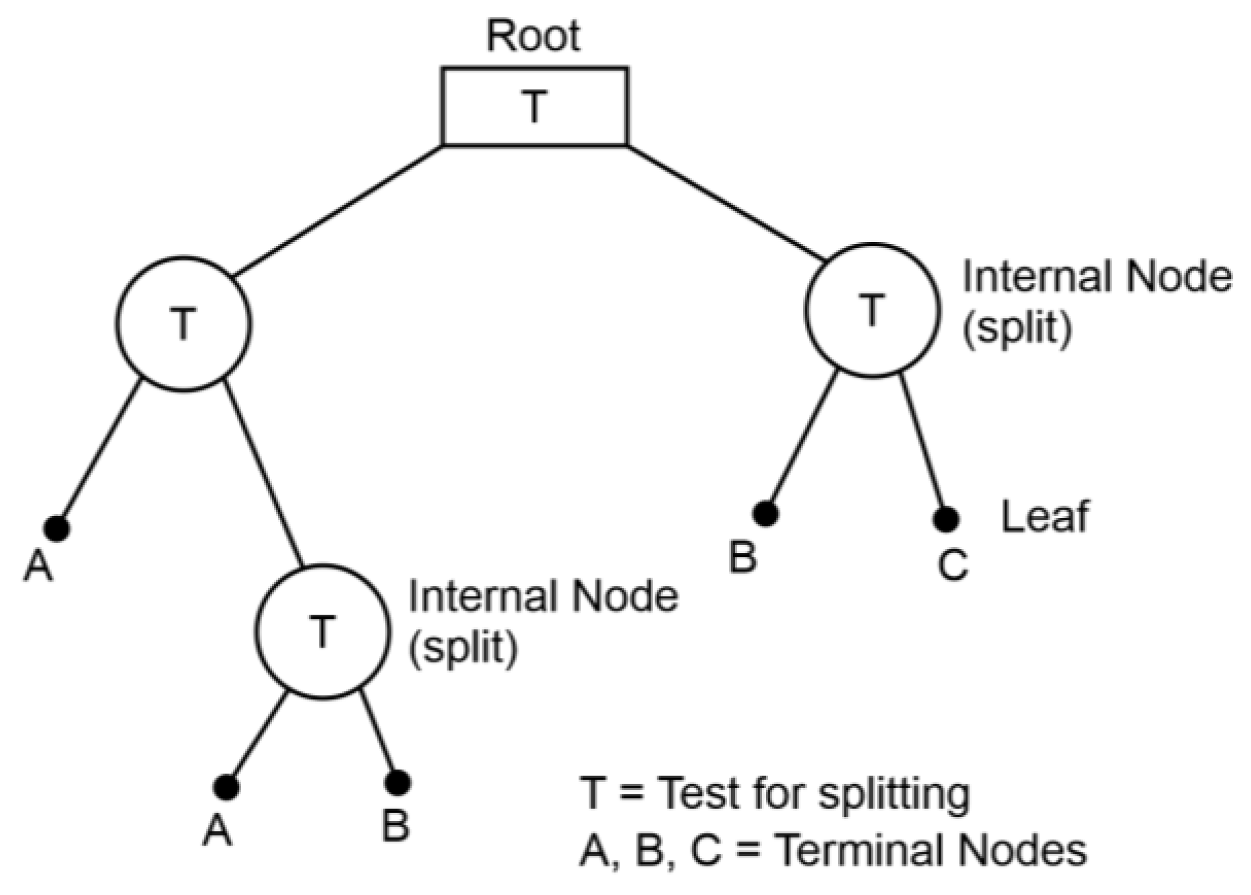
2.2. The Use of Machine Learning in the Models

This study employs machine learning approaches that utilize decision trees to provide a more accurate estimate of the death rate. Several articles, such as [12,17,18], have been published in the last decade on merging and improving these mortality models using machine learning algorithms. Machine learning algorithms can find trends in data and factors that mortality models may be unable to discern, and they may enhance the accuracy of fitting mortality models into samples and expected mortality. This study employs the decision tree technique because it is simple to understand and can detect non-linear and complex patterns. The method is unlike the random forest technique, which requires a long computation time and the artificial neural network technique, which requires large datasets to function adequately. Furthermore, this study uses classification and regression trees (CART) decision tree.

CART is a simple but powerful analytical tool that determines the most “important” variables based on their explanatory power in a dataset, and then constructs potent explanatory models. The determination process is carried out through a simple tree, which is divided into two techniques: classification and regression.

Process classification trees are used in CART for response variables that have classes or binary responses. Classification trees divide the data based on the homogeneity of the data; filtering out the “noise” makes it more “pure”, so the concept is called the purity criterion. However, regression trees are used for the numeric and continuous response variable, and the system development purpose is to use the data to predict outcomes. The regression model fits each independent variable and is used to divide variables based on nodes, which can reduce errors or residues from the model [19]. The CART structure can be seen in Figure 1.

The premise of this process is simple, given factors $x_1,x_2,x_3,\dots ,x_n$ in domain X, which is used to predict the response variable Y. In the picture above, the graphic is the domain of all factors associated with Y. CART is an alternative approach in developing models where the data are separated into pieces and where the interaction of variables is getting clearer. Mathematically, the challenge is to find a function d(x) that provides a one-to-one map of each point in X to a point in Y. The criterion for choosing d(x) is usually mean squared prediction error $E{\left\{d\left(x\right)-E(y|x)\right\}}^2$ for regression, or the expected cost for misclassification [20].

2.3. Externally Studentized Deviance

Residuals are the core of most diagnostic methods, and they are often utilized to analyze the quality of fit of mortality models. The deviance residuals have previously been used by [8] and [21,22,23], considering that the residual patterns could imply that the model does not satisfactorily describe all the data characteristics. For binomial random component, the scaled deviance residuals are defined as below.

$$r_{x,t}=sign\left(d_{x,t}-{\widehat{d}}_{x,t}\right)\sqrt{2\left[d_{x,t}\log \left(\frac{d_{x,t}}{{\widehat{d}}_{x,t}}\right)+\left(l_{x,t}-d_{x,t}\right)\log \left(\frac{l_{x,t}-d_{x,t}}{l_{x,t}-{\widehat{d}}_{x,t}}\right)\right]}$$

(7)

where $d_{x,t}$ indicates the number of deaths observed in the data, ${\widehat{d}}_{x,t}$ is the deaths expected by the model, and $l_{x,t}$ is the number of people living at the start of the indicated age interval. Although deviance residuals are usually symmetrical, their variance and thus their scale, are not standard. Thus, to rectify these situations, deviance residuals can be standardized using externally studentized deviance, which is defined by:

$$t_i=\frac{r_{x,t}}{\sqrt{S_{\left(i\right)}^2\left(1-h_{ii}\right)}}$$

(8)

The studentized deviance residuals are distributed by a standardized normal distribution when the fitted model is suitable. For this reason, these studentized residuals will generally lie between −3 and 3. Additionally, these residuals satisfy the assumptions of the Hotelling T2 control charts. By these, the studentized deviance residuals were utilized to check the mortality trend [24].

2.4. Hotelling T² Control Chart

By examining historical data, multivariate control charts are used to determine whether several variables or processes have been under statistical control. Hotelling proposed a T² control chart to monitor more than one variable simultaneously. Under the belief that the vector $X={\left(X_1,X_2,\dots ,X_p\right)}^{\prime }$ follows a p-variate normal distribution, with known covariance matrix Σ and mean vector $\mu ={\left({\mu }_1,{\mu }_2,\dots ,{\mu }_p\right)}^{\prime }$, the statistics are as follows:

$$T^2={\left(X-\mu \right)}^{\prime }{\mathsf{\Sigma }}^{-1}\left(X-\mu \right)$$

(9)

is distributed as a chi-square distribution with p degrees of freedom [25]. According to [26], using estimated μ and Σ, the Hotelling T² statistics are as follows:

$$T^2={\left(X-\overline{X}\right)}^{\prime }{\mathrm{S}}^{-1}\left(X-\overline{X}\right)~\frac{{\left(m-1\right)}^2}{m}{B}_{\left(p/2,\left(m-p-1\right)/2\right)}$$

(10)

where $B_{\left(p/2,\left(m-p-1\right)/2\right)}$ represents a beta distribution with parameters p/2 and (m−p−1)/2. This distribution depends on the total number of variables p and the sample size m, which must comply with the restriction, m > p +1.

Two phases must be passed, namely phase I and phase II. The purpose of phase I is to obtain a set of observations that are in control, while phase II is used to monitor future processes. Phase I analysis is also known as a retrospective analysis. In phase I, the upper control limit (UCL) is as follows.

$$UCL=\frac{{\left(m-1\right)}^2}{m}{B}_{\left(p/2,\left(m-p-1\right)/2\right)}.$$

(11)

The first step in phase I is to calculate UCL, and then plot the T² Hotelling statistics for each observation to obtain a phase I control diagram. When a point exceeds UCL, then the point is translated as a signal of shift in the distribution of X. Then, it is necessary to further investigate the cause of the signal through specific procedures to pinpoint the variable(s) causing the signal, because the T² control chart cannot show the specific causal variables that points to the signal.

This study uses the p-dimensional vector of an externally studentized deviance residuals $R_t={\left(st{r}_{1t},st{r}_{2t},\dots ,st{r}_{xt},\dots ,st{r}_{pt}\right)}^{\prime }$ as an indicator in monitoring changes in mortality dynamics obtained from the LC, RH, and CBD models for a reference sample of m successive periods (t = 1,2, 3, …, and m) so that the Hotelling T² statistics are obtained as:

$$T^2={\left(R-\overline{R}\right)}^{\prime }{\mathrm{S}}_{\mathrm{R}}^{-1}\left(R-\overline{R}\right)$$

(12)

3. Implementation: Mortality Modelling

3.1. Fitting Lee–Carter Model

The initial part of this study compares the model formed from the parameter estimation process when the setting is either Poisson or Quasi-Poisson. Furthermore, the model with the Quasi-Poisson setting, which was previously used by [8], is called LC1, and the proposed model in this research with the Poisson setting is denoted with LC2. By using the same data as in [8], this current study tries to use a more commonly used model that complies to popularly reported parameter constraints.

The data are from Colombia for 1973–2005, with both male and female populations obtained from “The Latin America Human Mortality Database” [27]. The data on the living population ($l_{x,t}$) available are only the collected data at the time of the census, namely 1973, 1985, 1993, and 2005, while interpolation is carried out between the years in this database. Additionally, the population was grouped into age groups 0, 1–5, 5–10, 10–15, and so on up to 80–85 years for each sex.

The parameter estimation process in both models was carried out with the statistical software R, where LC1 models can be fitted using the gnm package [28]. In contrast, LC2 was carried out with the StMoMo package [24]. The results of estimating the parameters of the two models can be seen in Figure 2.

The estimation results of the two parameters related to the age-specific models, LC1 and LC2, showed the same results, but the parameters related to the period t showed different results. The LC1 model used in the research by [8] shows the value of ${\kappa }_t^{\left(1\right)}$ starting from 0, while the LC2 model can meet the constraints specified in the model parameterization, namely ${\displaystyle \sum }_t{\kappa }_t^{\left(1\right)}=0$.

Furthermore, to compare the results of the two models, the performance model is assessed with three measures: the deviance, the mean absolute percentage error (MAPE), and the mean square error (MSE). The first measure is a distance between the observed $q_{x,t}$ and the adjusted values ${\widehat{q}}_{x,t}$, whose expression is as follows:

$$D\left({\widehat{q}}_{x,t}\right)=2logL\left(q_{x,t}\right)-2logL\left({\widehat{q}}_{x,t}\right)$$

(13)

where log L(.) is the binomial log-likelihood function because the number of deaths is assumed to be distributed as a binomial. Used by [29], the second [29] is defined by the following equation:

$$MAPE\left({\widehat{q}}_{xt}\right)=\frac{{{\displaystyle \sum }}_x\frac{\left|q_{xt}-{\widehat{q}}_{xt}\right|}{q_{xt}}}{n},t=1,2,\dots ,T$$

(14)

MAPE measures the mean absolute error weighted with the inverse of the crude estimates $q_{xt}$. These weights allow us to decrease the effect of the errors associated with bigger values of $q_{xt}$, which are usually associated with intermediate and advanced age groups. The third is defined by the following equation:

$$MSE\left({\widehat{q}}_{xt}\right)={\displaystyle \sum }_x\frac{{\left(q_{xt}-{\widehat{q}}_{xt}\right)}^2}{n},t=1,2,\dots ,T.$$

(15)

MSE measures the error in estimations without any adjustment. The value of these three measures of the goodness-of-fit is shown in

Table 1. Performance of LC1 and LC2 models.

		Model
		LC1	LC2
Deviance	Female	872549.4	1614.1
	Male	627047.6	14261.2
MSE	Female	1968.57	370.71
	Male	2500.44	532.95
MAPE	Female	0.42938	0.06283
	Male	0.37023	0.08015

.

Table 1 shows that the Lee–Carter mortality model with the Poisson setting (LC2) produces a better model than Quasi-Poisson (LC1 which was proposed by [8]), through lower MSE and MAPE indicators. The model with the Poisson setting can also meet the constraints set previously. It can be concluded that for the LC model, it is more appropriate to use the Poisson setting than the Quasi-Poisson to achieve more optimal results.

3.2. Fitting LC, RH, and CBD Models

After knowing the approach that will obtain the best LC model, namely the Poisson setting, we used this approach for the following analysis. The next step is to use the mortality data from several countries in projecting the mortality rates using three mortality models, namely the Lee–Carter (LC), the Renshaw–Haberman (RH), and the Cairns–Blake–Dowd (CBD). The performance of the three models were compared using two measures, namely the mean absolute percentage error (MAPE) and the mean square error (MSE).

The data used are the Japanese population data from the Human Mortality Database [30], which contains data on the deaths from countries in the world over a relatively long period. Single-age data ranging from 0 to 100 were used to estimate the model parameters.

The LC, RH, and CBD models are fitted to the Japanese population data. The parameters of the LC, RH and CBD models fitted to the mortality population data can be found in Figure 3, Figure 4 and Figure 5, respectively, for both males and females. The parameters for the three mortality models were explained in the previous section. Parameter ${\alpha }_x$ is the age function and represents the average level of mortality at each age, ${\beta }_x^{\left(1\right)}$ represents the response at each age to the change in mortality over the years, ${\kappa }_t^{\left(1\right)}$ is the period index that represents the mortality level each year, and ${\gamma }_{t-x}$ is the cohort index representing the cohort effect.

The ages in the graphs range from 0 to 100, the years range from 0 to 74, representing the years 1947 to 2020, and the cohorts range from 0 to 174, representing the “birth” years from 1847 to 2020 for each cohort group, which was found retrospectively, 100 years after the first-year interval in the study.

From Figure 3, there are three parameters in the Lee–Carter model, which are ${\alpha }_x$, ${\beta }_x^{\left(1\right)}$, and ${\kappa }_t^{\left(1\right)}$, which show many similarities for males and females. The graph of the age function parameter ${\alpha }_x$, which represents the average level of mortality at each age, roughly shows the same mortality trends over different ages for both sexes. At zero, the mortality rate starts relatively high, and then it decreases until the age of ten. From the age of 10 until 90, the mortality rate increases, approximately linearly, except for the small spike around 20 caused by accidental deaths. So, the age function parameter for the LC model shows an increasing trend after approximately 20 years. Keeping all other parameters constant would mean that the central death rate is also increasing after the age of approximately 20.

The parameter ${\beta }_x^{\left(1\right)}$, which represents the response at each age to the change in mortality over the years for males and females starts high and is relatively volatile for younger ages. The ${\beta }_x^{\left(1\right)}$ represents the sensitivity of the ages to the changes in mortality over the years. This means that the younger ages are more sensitive to the changes in mortality over the years than the older ages. After approximately 50 years, the ${\beta }_x^{\left(1\right)}$ increases slightly until approximately 75 years, and then decreases almost linearly until the age of 90.

The graph of the period index, which represents the mortality level each year, ${\kappa }_t^{\left(1\right)}$ shows a decreasing trend over time. The further we go into the past, the higher the mortality level is for each year. It can also be seen that the mortality level in each year before 1985 for females is higher than the mortality level in the corresponding years for males. Keeping all other parameters constant would mean that the central death rate would also decrease each year.

The parameters of the RH model show some similarities to the parameters of the LC model. The age function parameter, ${\alpha }_x$, also increases when age increases. Keeping all other parameters constant, the central death rate increases per age, which is expected. The period index, ${\kappa }_t^{\left(1\right)}$, again shows a decreasing trend, which is logical as t indicates the mortality level each year. As seen in Figure 4, the central death rates for all ages decrease until approximately 1985. After that, the rates increase until 2020.

The ${\gamma }_{t-x}$ represents the cohort effect, linking the mortality levels to a generation born in a specific year. In the graphs of ${\gamma }_{t-x}$, there is an increasing trend until the cohort of approximately year 1875 for males and year 1880 for females, and a decreasing trend afterwards. This means that the mortality levels for the generations born until 1875 for males and 1880 for females are increasing, and the mortality levels for the generations of males born after 1875 and females born after 1880 are decreasing.

This demographic phenomenon can be explained as related to some historical conditions. The presence of World War II and the Japanese War can also be seen in the graph of ${\gamma }_{t-x}$ for males, as values for ${\gamma }_{t-x}$ increase up until approximately 1875, indicating higher mortality levels for the generations of males born between 1850 and 1875, which include males who fought in World War II. In addition, the discovery of penicillin can also indicate the cause of a significant trend in the Japanese population. Keeping all other parameters constant, as ${\gamma }_{t-x}$ decreases, the central death rate also decreases. So, after the cohort of 1875 for males and 1880 for females, ${\gamma }_{t-x}$ shows a decreasing trend indicating that the central death rate also decreases.

In the CBD model, the value of $\left(x-\overline{x}\right)$ significantly impacts logit ($q_{xt}$), so the age group used in estimating the parameters will affect the rates of mortality. The estimation results of the two CBD model parameters show different trends. ${\kappa }_t^{\left(1\right)}$ shows a trend that continues to decline, with the female population below the male population with an increasing gap.

In contrast, the second parameter shows an increasing trend, with the female population located higher than the male population. The CBD mortality index, ${\kappa }_t^{\left(2\right)}$, denotes the level of the mortality curve (the curve of $q_{xt}$ in year t) following a logit transformation. A reduction in ${\kappa }_t^{\left(2\right)}$ and a parallel downward change of the logit-transformed mortality curve, represents a global mortality improvement. The Japanese data in Figure 5 show that the mortality improvement in the male population is relatively better than that of the female population.

Furthermore, the three models are compared using the mean square error (MSE) and the mean absolute percentage error (MAPE) in

Table 2. Performance of three models before and after the DT.

		Model before DT			Model after DT
		LC	RH	CBD	LC	RH	CBD
MSE	Female	1,015,645	142,174	14,369,727	112,582	36,499	1,461,146
	Male	716,095	265,295	15,412,708	94,242	62,945	1,278,129
MAPE	Female	0.1634	0.0625	0.4363	0.0639	0.0437	0.1679
	Male	0.0968	0.0646	0.3596	0.0504	0.0409	0.1697

. The result of the machine learning technique decision tree (DT) process that has been carried out at this stage is also seen as a measure of its performance.

The machine learning process results show an optimization of the model, by showing lower MSE and MAPE values than the model without machine learning with the decision tree (DT). The decision tree implementation is based on two criteria, namely years and cohorts, from which the data are taken to produce a CART (classification and regression tree) regression tree. The first step is to construct the decision tree process through the sum of squared errors with optimal iterations, where the recursive process is stopped when the number of observations is less than six. From there, response estimators can be obtained using the data for the analysis process. Then, of the three models that have been formed, the RH model shows the lowest MSE and MAPE numbers, indicating that the RH model for projecting mortality rates in Japan is the best model that can be chosen compared to the other two models, namely LC and CBD.

4. Analysis of the Multivariate Control Chart

4.1. Hotelling T² Control Chart

The Hotelling T² control chart was retrospectively used to pinpoint substantial mortality changes during the study period that the best mortality model did not address. Information on these unmodeled changes is observed in the model residuals. In this application, the residual for each specific age interval is considered a random variable. In this way, the p residuals of the mortality model make up a vector of random variables but, in practice, they are not necessarily independent.

Tests using control charts were carried out for all countries in the Human Mortality Database. In total, there are 41 countries tested in this study using a multivariate control chart, which have multivariate normal distributed data, to see how the control chart performs when comparing the three mortality models. All test results show the same findings; namely, the RH model has more signals than the other two models, both before applying the machine learning techniques and after. This shows that the RH model has a higher level of sensitivity than the other two models in detecting substantial changes in the model residuals.

In addition, several countries such as Norway, Belgium, Canada, and Japan also showed similar results to Figure 6. No signal was detected in the LC or CBD models when we set α = 0.001 (or only detected in one gender), but the RH model control chart was able to provide signals for both sexes.

These results show that the RH model is good at projecting the mortality rates in a country. So, further analysis can be carried out regarding the years that obtain signals in the control chart. This decomposition study will be carried out in Saudi Arabia in the next subsection.

4.2. Decomposition of The Residuals to Explore Specific Age Groups

This study uses the Saudi Arabian population dataset to model the mortality rate using the Renshaw–Haberman (RH) mortality model. Saudi Arabia’s population and mortality data were obtained from the World Bank data, with adjustments from the results of the census by the General Authority for Statistics (GAStat) of Saudi Arabia. The period taken for the study is 1990 to 2021, with age groupings from 0–1, 1–5, 5–9, 10–14, …, and 85+.

After the model was built with the application of machine learning techniques, the externally studentized deviance residuals were entered as inputs in the multivariate control charts. The results of the Hotelling T² control chart in Figure 7 were obtained for the male and female populations. Signals in the male population were recorded more than in the female population, namely four and two signals, respectively. Furthermore, in the specific year that shows the signal on the control chart, the T² value is decomposed to take a deeper look at the signal so that substantial changes can be monitored in the residuals.

In summary, the Hotelling T² control chart for the RH model indicates that both sexes were out of control in 1991. Additionally, the Hotelling T² control chart for the RH model identifies 2015 for females, and identifies 1996, 2001, and 2003 for males. Here, the out-of-control signal should be considered a shift that the RH mortality model could not account for. Therefore, in the absence of out-of-control signals, it should not be assumed that the chart indicates no changes in mortality. Rather, it should be assumed that these changes are most likely already accounted for by the model.

For the out-of-control signals, the ages responsible for the signals are investigated by applying the decomposition.

Table 3. T² values for the signals.

Sex	Year	T2 Values 1
Female	1991 2015	24.84 25.86
Male	1991 1996 2001 2003	26.81 25.89 26.96 25.76

¹ α = 0.001 and UCL = 24.67.

summarizes the information obtained from the absolute term of the decomposition of signaling points for the residual vector of RH models.

There are several methods to interpret the multivariate signal. Research by [26] proposed the MTY decomposition method for determining the origins of signals. Hotelling’s T² statistic is decomposed by the MTY technique into p additive orthogonal components, each of which indicate the contribution of distinct process variables as well as the relative joint contribution of the same process variable.

For both sexes, the residuals of the mortality model point to 1991 as beyond the limits of control, where infants and the elderly mainly cause this alarm (cf.

Table 4. Unconditional terms of the MTY decomposition for out-of-control points.

Age Group	Female		Male
	1991	2015	1991	1996	2001	2003
0–1	3.70 *	0.83	3.87 *	3.89 *	3.09 *	0.27
1–4	1.20	0.85	1.00	0.99	0.24	2.33
5–9	0.07	1.28	0.14	0.50	0.57	0.18
10–14	1.56	0.41	3.09 *	4.89 *	0.40	0.27
15–19	0.57	0.87	0.61	1.03	0.76	0.10
20–24	0.93	1.40	0.06	2.13	1.39	1.28
25–29	0.61	3.89 *	1.28	1.33	0.40	1.56
30–34	0.18	0.38	0.41	0.44	0.07	1.36
35–39	0.91	0.39	0.39	0.56	0.83	0.80
40–44	0.18	2.96 *	1.75	0.69	3.86 *	0.71
45–49	1.96	1.29	0.59	0.83	0.02	5.08 *
50–54	1.71	1.27	0.01	1.61	1.42	5.31 *
55–59	0.56	0.24	0.17	0.62	1.11	0.20
60–64	1.53	0.54	0.09	0.40	0.04	0.59
65–69	1.18	0.76	1.21	0.25	0.34	0.33
70–74	3.23 *	1.95	2.79 *	0.42	0.82	2.63 *
75–79	0.06	0.78	1.21	0.58	1.44	0.95
80–84	0.68	0.25	3.18 *	0.54	0.45	0.68
85+	3.74 *	0.19	2.46 *	3.47 *	0.48	2.32

* Denotes significance with α = 0.10 and UCL = 2.45.

). However, in 2015 for females and in 2001 or 2003 for males, the signal was shown in the productive age group. This indicates a shift in the model error that can be caused by specific parameterization characteristics or due to certain unmodelled demographic conditions.

5. Conclusions

Our paper aims to reveal and confirm substantial cohort changes in three mortality models. To this end, we propose the multivariate control chart, Hotelling T², for monitoring the signal. We obtain the externally studentized deviance after fitting the model, and optimization of the model is achieved using decision tree machine learning techniques. To the best of our knowledge, this is the first piece of work that constructs the exact mortality modelling that satisfied all the model constraints and combined machine learning techniques with control chart monitoring. The proposed method is applied to study the mortality in a country with limited data, especially in developing countries, as well as early warnings for forecasting mortality changes.

References

1. Cox, P.R. Demography; Cambridge University Press: Cambridge, MA, USA, 1976. [Google Scholar]
2. Embrechts, P.; Wüthrich, M.V. Recent challenges in actuarial science. Annu. Rev. Stat. Its Appl. 2022, 9, 119–140. [Google Scholar] [CrossRef]
3. Zili, A.H.A.; Kharis, S.A.A.; Lestari, D. Peramalan tingkat kematian Indonesia akibat COVID-19 menggunakan model ARIMA. J. Indones. Sos. Sains 2021, 2, 1–8. [Google Scholar] [CrossRef]
4. Gompertz, B. XXIV. On the nature of the function expressive of the law of human mortality, and on a new mode of deter-mining the value of life contingencies. In a letter to Francis Baily, Esq. FRS & c. Philos. Trans. R. Soc. Lond. 1825, 115, 513–583. [Google Scholar]
5. de Moivre, A. Annuities upon Lives, or, the Valuation of Annuities upon Any Number of Lives, as Also, of Reversions: To Which Is Added, an Appendix Concerning the Expectations of Life, and Probabilities of Survivorship; Oxford University: London, UK, 1731. [Google Scholar]
6. Weibull, W. A Statistical Theory of the Strength of Materials; Generalstabens Litografiska Anstalts Förlag: Stockholm, Sweden, 1939. [Google Scholar]
7. Luy, M.; di Giulio, P.; di Lego, V.; Lazarevič, P.; Sauerberg, M. Life expectancy: Frequently used, but hardly understood. Gerontology 2020, 66, 95–104. [Google Scholar] [CrossRef]
8. Díaz-Rojo, G.; Debón, A.; Mosquera, J. Multivariate control chart and Lee–Carter models to study mortality changes. Mathematics 2020, 8, 2093. [Google Scholar] [CrossRef]
9. García-Bustos, S.; Cárdenas-Escobar, N.; Debón, A.; Pincay, C. A control chart based on Pearson residuals for a negative binomial regression: Application to infant mortality data. Int. J. Qual. Reliab. Manag. 2021, 39, 2378–2399. [Google Scholar] [CrossRef]
10. AKoetsier; de Keizer, N.; de Jonge, E.; Cook, D.; Peek, N. Performance of risk-adjusted control charts to monitor in-hospital mortality of intensive care unit patients: A simulation study. Crit. Care Med. 2012, 40, 1799–1807. [Google Scholar] [CrossRef]
11. Felix-Cardoso, J.; Vasconcelos, H.; Rodrigues, P.; Cruz-Correia, R. Excess mortality during COVID-19 in five European countries and a critique of mortality data analysis. MedRxiv 2020. [Google Scholar] [CrossRef]
12. Deprez, P.; Shevchenko, P.; Wüthrich, M.V. Machine learning techniques for mortality modeling. Eur. Actuar. J. 2017, 7, 337–352. [Google Scholar] [CrossRef]
13. Lee, R.D.; Carter, L.R. Modeling and Forecasting U. S. Mortality. J. Am. Stat. Assoc. 1992, 87, 659. [Google Scholar] [CrossRef]
14. Renshaw, A.; Haberman, S. A Cohort-Based Extension to the Lee–Carter Model for Mortality Reduction factors. Insur. Math. Econ. 2006, 38, 556–570. [Google Scholar] [CrossRef]
15. Haberman, S.; Renshaw, A. A comparative study of parametric mortality projection models. Insur. Math. Econ. 2011, 48, 35–55. [Google Scholar] [CrossRef] [Green Version]
16. Cairns, A.J.G.; Blake, D.; Dowd, K. A Two-Factor Model for Stochastic Mortality with Parameter Uncertainty: Theory and Calibration. J. Risk Insur. 2006, 73, 687–718. [Google Scholar] [CrossRef]
17. Hong, W.H.; Yap, J.; Selvachandran, G.; Thong, P.; Son, L.H. Forecasting mortality rates using hybrid Lee–Carter model, artificial neural network and random forest. Complex Intell. Syst. 2021, 7, 163–189. [Google Scholar] [CrossRef]
18. Levantesi, S.; Pizzorusso, V. Application of Machine Learning to Mortality Modeling and Forecasting. Risks 2019, 7, 26. [Google Scholar] [CrossRef] [Green Version]
19. Morgan, J. Classification and Regression Tree Analysis; Boston University: Boston, MA, USA, 2014; Volume 298. [Google Scholar]
20. Loh, W.-Y. Fifty years of classification and regression trees. Int. Stat. Rev. 2014, 82, 329–348. [Google Scholar] [CrossRef] [Green Version]
21. Coelho, E.; Nunes, L.C. Forecasting mortality in the event of a structural change. J. R. Stat. Soc. Ser. A Stat. Soc. 2011, 174, 713–736. [Google Scholar] [CrossRef]
22. Debón, A.; Montes, F.; Puig, F. Modelling and forecasting mortality in Spain. Eur. J. Oper. Res. 2008, 189, 624–637. [Google Scholar] [CrossRef] [Green Version]
23. Renshaw, A.; Haberman, S. On simulation-based approaches to risk measurement in mortality with specific reference to Poisson Lee–Carter modelling. Insur. Math. Econ. 2008, 42, 797–816. [Google Scholar] [CrossRef] [Green Version]
24. Villegas, A.; Kaishev, V.; Millossovich, P. StMoMo: An R package for stochastic mortality modelling. In Proceedings of the 7th Australasian Actuarial Education and Research Symposium, Queensland, Australia, 3 December 2015. [Google Scholar]
25. Hotelling, H. Techniques of Statistical Analysis. In Chapter Multivariate Quality Control Illustrated by the Testing of Sample Bombsights; McGraw-Hill: New York, NY, USA, 1947; pp. 113–184. [Google Scholar]
26. Tracy, N.D.; Young, J.C.; Mason, R.L. Multivariate Control Charts for Individual Observations. J. Qual. Technol. 1992, 24, 88–95. [Google Scholar] [CrossRef]
27. Urdinola, B.P.; Torres, F.; Velasco, J.A. Latin American Human Mortality Database. 2022. Available online: www.lamortalidad.org (accessed on 23 October 2022).
28. Turner, H.; Firth, D. Generalized Nonlinear Models in R: An Overview of the Gnm Package; University of Warwick: Coventry, UK, 2007. [Google Scholar]
29. Adebón; Martínez-Ruiz, F.; Montes, F. A geostatistical approach for dynamic life tables: The effect of mortality on re-maining lifetime and annuities. Insur. Math. Econ. 2010, 47, 327–336. [Google Scholar]
30. Jdanov, D.A.; Jasilionis, D.; Shkolnikov, V.; Barbieri, M. Human Mortality Database; Max Planck Institute for Demographic Research: Rostock, Germany; University of California: Berkeley, CA, USA; French Institute for Demographic Studies: Paris, France, 2019. [Google Scholar]
Figure 1. The structure of the CART.
Mathematics 11 00566 g001
Figure 2. Parameter plot for LC1 and LC2 models for both male (solid line) and female (dashed line). Note that model LC1 is denoted by (a,c,e), while model LC2 is denoted by (b,d,f).
Mathematics 11 00566 g002
Figure 3. Japan’s LC model for both males (solid line) and females (dashed line).
Mathematics 11 00566 g003
Figure 4. Japan’s RH model for both male (solid line) and female (dashed line).
Mathematics 11 00566 g004
Figure 5. Japan’s CBD model for both male (solid line) and female (dashed line).
Mathematics 11 00566 g005
Figure 6. Hotelling T2 control charts for all models after DT.
Mathematics 11 00566 g006aMathematics 11 00566 g006b
Figure 7. Hotelling T2 control charts.
Mathematics 11 00566 g007