Article

Deterioration Control Decision Support System for the Retailer during Availability of Trade Credit and Shortages

1
Department of Applied Sciences, Faculty of Engineering and Technology, Parul University, Vadodara 391760, Gujarat, India
2
Department of Mathematics, M. G. Science Institute, Gujarat University, Ahmedabad 380009, Gujarat, India
3
Prestige Institute of Management and Research, Gwalior 474020, Madhya Pradesh, India
4
Government Polytechnic Dahod, Dahod 389151, Gujarat, India
5
Electrical Engineering Department, College of Engineering, King Khalid University, Abha 61421, Saudi Arabia
6
Computers and Communications Department, College of Engineering, Delta University for Science and Technology, Gamasa 35712, Egypt
7
Computer Engineering Department, College of Computer Science, King Khalid University, Abha 61421, Saudi Arabia
*
Author to whom correspondence should be addressed.
Mathematics 2023, 11(3), 580; https://doi.org/10.3390/math11030580
Submission received: 30 November 2022 / Revised: 6 January 2023 / Accepted: 9 January 2023 / Published: 21 January 2023
(This article belongs to the Topic Mathematical Modeling)

Abstract

:
The deterioration rate is a significant aspect of perishable goods. Since perishable items will always deteriorate, there are effective methods for reducing the rate of deterioration. Furthermore, in the existing inventory control literature, the deterioration rate is often viewed as an exogenous component. Keeping this problem in mind, this article develops the perishable inventory control system from the retailer’s perspective in which: (i) the deterioration rate is a controllable factor and suggests a new fresh quality technology (FQT) indicator, (ii) demand is determined by the perishable product’s quality, that is controlled by its rate of deterioration, (iii) the credit duration is predefined, and (iv) shortages are expected. The key goal is to demonstrate that there is an ideal quantity of the order that minimizes the retailer’s overall cost in terms of cycle time and deterioration rate. Finally, theoretical results are validated by solving two numerical illustrations and conducting a sensitivity analysis of the main factors resulting from the following managerial implications: (i) if the range of deterioration is between zero and one then the retailer should invest in the preservation factor to preserve the perishable product and if greater than one the retailer should not invest in the preservation factor, (ii) credit period significantly reduces the total cost. Hence, this trade credit strategy is more beneficial to the model.

1. Introduction

In real-world scenarios, the deterioration of products is a big issue in every business segment. As perishable goods transit through a supply chain, they deteriorate at different rates. Farming products such as fruits, vegetables, and meat are examples of perishable products. Uncontrolled deterioration results in a large amount of spoiling waste. The loss ratio due to the deterioration of fresh produce is as high as 30% in many countries [1]. In China, the annual loss of agricultural products amounts to more than USD 43 billion, which is equivalent to the production output of 0.1 billion hectares of cultivated land (China Economic Information Daily 2016). Recent advanced technologies such as the freshness preservation effort (FPE) [2], fresh-keeping effort (FKE) investment strategies, and a fresh product supply chain (FSC) system [3] have resulted in the development of emerging innovations that may be utilized efficiently to assess and control the rate of deterioration [4]. In general, the rate of deterioration (DR) calculates the proportion of perishable items that are unusable due to decay or expiry [5]. For illustration, fresh vegetables have a different DR depending on the storage climate and handling techniques. Furthermore, the rate of deterioration of the most perishable items remains constant under constant environmental conditions but begins to fluctuate when storing temperature and humidity change. Because a perishable product’s deterioration rate is proportional to its quality, it has a significant impact on sales [3]. The availability of fresh goods on display affects sales at the point of purchase [2]. Due to the general significant visual aspects of the farming quality of the product and stock, the consumption trend and, as a result, inventory management of agricultural products differs from those for other perishable goods.
Since a perishable item’s rate of deterioration may be reduced by proper handling and storage environments, it should be evaluated as a decision parameter when circumstances permit. As a result, the appropriate inventory strategy can be controlled using both freshness-dependent demand and deterioration control information. Hence, to support deterioration rate management, this article suggests a unique fresh quality technology (FQT) parameter. Investing in suitable technology and manpower to furnish needed storage and handling conditions, on the other hand, loss of farming goods due to a lower rate of deterioration. The reduced degradation rate of farming goods justifies the high investment cost for effective inventory management. Although loss prevention is an important aim in farming product inventory control, economic concerns are a primary focus for real-world retail decision making. Therefore, in this model, deterioration rate is controllable and considered as a decision variable with the effort of freshness technologies and quality.
In this modern dynamic and competitive business context, trade credit policy becomes one of the most appropriate and efficient strategies to enhance demand and control commodities. If a supplier offers a retailer to pay for products later without incurring interest costs, the retailer is more inclined to purchase commodities. Therefore, the supplier provides the retailer with a specific time to make the payment. This type of business finance in which the retailer is permitted to purchase goods and pay the supplier afterward is identified as a trade credit policy [6]. Many companies use this strategy to increase sales and attract more customers. In addition, when a product’s demand frequently increases because of the quality and freshness but the product is unavailable for a sustained duration, shortages arise. Therefore, this article permits the partially backlogged shortages when the cycle time comes to an end and also considers the upstream credit period in which the supplier offers a retailer a mutual credit time so that the retailer can pay the balance at a later scheduled date; this realistic scenario forms the basis of this study.

1.1. Aim of This Study

The objective of this research is to go into a new realm such as the field of inventory management for agricultural products. The following important interesting and significant questions are examined in this research:
  • What is the need for controlling deterioration rate using fresh quality technology and effort according to a cost factor?
  • Why does the deterioration rate always consider the ideal rate if the deterioration rate is between 0 and 1?
  • Why must the optimal rate of deterioration and preservation factor be in the interval [ 1 , + ) ?
  • How does a strategy of trade credit affect a retailer’s productivity and profitability?
  • When should a retailer have to place a back order to escape stock-outs?
  • If this model were implemented in reality, what would the managerial implications be?

1.2. Contribution

Perishable products have high and varying deterioration rates when passing through their logistics systems. Agri-fresh products are a typical example of perishable products that include fresh fruits, fresh vegetables, and fresh meat. This article models the perishable inventory decision support system [7] with deterioration-controlled/freshness-dependent demand, and quality indication. Additionally, the allowable shortages condition, trade credit policy, and controllable deterioration rate are used to analyze the dynamics with various scalable parameters. We analytically model this scenario and perform sensitivity analysis to generate associated managerial implications. The most significant contributions are summarized below:
  • This study develops a perishable inventory system in which deterioration rate is considered as a decision parameter and investigates its impact on perishable quality control parameters.
  • The rate of deterioration is controlled using the fresh quality technique and effort as a cost factor.
  • The demand depends on the deterioration and quality of the perishable product.
  • Quality is defined as the time integration of the original and deteriorating quality. For illustration, a farming product with a reduced deterioration rate, which appears fresh and has much more available stock, will generate higher demand.
  • Trade credit policy and its impact on the overall cost of the retailer.
  • Partially backlogged shortages are permitted.

1.3. Flow of the Paper

The remaining portion of this article is discussed as follows: Section 2 is the existing review of the literature. In Section 3, the notation and assumptions are discussed. Section 4 creates a mathematical model for various upstream trade credit scenarios to minimize the overall cost of the retailer. After that, Section 5 contains the numerical study, the sensitivity analysis for the key parameters, and managerial implications for the retailer. Finally, Section 6 moderates the conclusion and future prospects for this article.

2. Literature Review

In this part, a review of the literature on product demand, deterioration, and trade credit policy in inventory models is used to highlight gaps in the area and demonstrate how prior works have contributed to this research. The first segment focuses on the literature on modeling techniques with demand, the second focuses on models with deteriorating items, and the third focuses on trade credit.

2.1. Literature Review on Inventory Models under Various Types of Demand

The most essential aspect of a business and enterprise is demand. The various forms of demand have been explored by researchers over the past few years. As a result, the researchers have taken into account various kinds of demand and developed inventory models. In this way, [8] represents a model for advertisement-dependent demand with a single-layered trade credit policy system. In [9], the authors prepared a mathematical model under the exponentially declining demand by using the concept of an allowable shortage. An economic order quantity (EOQ) model under time-linked quadratic demand with constant deterioration was introduced by [10]. Further, the perishable commodities inventory model with the preservation tool and price reduction problem under the stock- and price-dependent demand is explained by [11]. An EOQ model under the ramp demand for deteriorating products has been discussed in [12]. In recent times, a model with the consideration of shortages under the time and selling price-dependent demand has been established in [13]. An inventory model with a nonlinear stock-dependent demand for non-instantaneously deterioration is developed in [14]. After this, the role of trapezoidal demand in the inventory model for sustainable operations of fixed lifetime products is discussed in [15]. This study extends the work of [2], which proposed a controllable deterioration rate linked model for the deterioration-dependent demand. There is very little research that depends on the relationship between deterioration and demand. The contribution of this study is that the demand is completely reliant on the deterioration rate.

2.2. Literature Review on Inventory Models under Deteriorating Inventories

Since managing deteriorating inventory affects so many businesses, academics have published several articles to address the related difficulties in reality. Hence, the rate of deterioration is an important factor for describing the essential characteristics of perishable goods. Several products have a deteriorating nature over time such as fresh fruits and vegetables, milk, juice, any dairy product, etc. The retailer aims to control the amount of deterioration and stimulate demand. Therefore, the researchers took this into account and established models to reduce the rate of deterioration. The review of a perishable inventory since 2001 is reflected in [5]. Further, in [16], an inventory model under the quadratic demand by applying a maximum fixed lifetime deterioration rate is extended. A model with shortages for the constant deteriorating goods was derived by [17,18]. Furthermore, in [19], a mathematical model in which the rate of deterioration is non-instantaneous and demand is motivated by the price and stock of the product is derived. An inventory model for continuously deteriorating goods with the scheme of payment in advance was formulated by [20]. Later, a stock model for the time-dependent decline products under the demand which is sensitive to both time and price was determined by [21]. A model for controllable deterioration rate was developed by [22,23]. Further, the most significant contributions in this study were elaborated upon by [2] who established a controllable deterioration rate linked model. In [24], a concept related to the Weibull deterioration rate over the finite time perspective was established. Recently, the inventory model with green-level-dependent demand with constant deterioration has been derived in [25]. After this, [26] and others have contributed notable contributions to this field of research. Therefore, all of the researchers considered the various types of deterioration but this article focuses on the controllable deterioration rate of the perishable products.

2.3. Literature Review on Inventory Models under Trade Credit Policy

Many stock models are developed that assume payment is paid at the moment the order amount is received. However, in reality, the payment of purchase cost differs between the following: (i) payment on delivery received [27], (ii) acceptable partial payment delay, (iii) a partial deposit payment [28], and (iv) partial advance payment and allowing partial payment delay [29]. For example, a mathematical model for deteriorating products under a single-layered trade credit strategy is elaborated upon in [30]. Further, a stock model for time-dependent deteriorating goods under the two-layered partial trade credit scheme is developed in [31]. In [32], the impact of carbon emission of a supply chain under the two-layered trade credit policy is established. In addition, the partial backlogged shortages and multi-layered trade credit model are discussed in [33]. Additionally, a mathematical model under the price- and advertisement-dependent demand for a single-layered trade credit system was calculated in [34]. In this way, a stock model with two-layered trade credit and dynamic demand is incorporated in [35]. Lately, a model under the price-sensitive demand with investment in preservation equipment and single-layered trade credit policy has been created in [36]. Other inventory models include a trade credit strategy provided by [37,38,39]. Recently, the inventory model with partial linked-to-order upstream trade credit and downstream full trade credit has been developed by [40]. Moreover, Table 1 provides a concise description of the existing literature relevant to the proposed model.

2.4. Gap Identification

According to the literature survey and Table 1, several studies have worked on different combinations but the uniqueness of this research is that all of the combinations such as deterioration-dependent demand, controllable deterioration, allowable shortages, and trade credit policy which were previously not considered in any articles are examined. The work of [2] established an inventory model for the controllable rate of deterioration. In this model, they only focused on the deterioration of the perishable product. In contrast to [2], this article considers the fresh quality technology (FQT), trade credit policy, and allowable shortages. Furthermore, in the literature, many authors used different techniques to control the deterioration rate. The items deteriorate in nature as shown in [16]. To control the rate of deterioration, the authors developed some technologies such as freshness preservation effort (FPE) [2], fresh-keeping effort (FKE) investment strategies, and a fresh product supply chain (FSC) system [3], as well as the freshness-keeping effort of third-party logistics service providers (TPLSPs) [41]. This study significantly derives the relation between the fresh quality technology (FQT) indicator and the deterioration rate which is the novelty of this work.

3. Notation and Assumptions

Assumptions

The inventory system only applies to a single item.
The indicator of fresh quality technology (FQT) is γ = h θ h c , where h θ denotes the controllable marginal cost of holding with preservation and h c is the maximum cost of holding including preservation which denotes the highest-level effort of h θ . Additionally, 0 < h θ < h c and when h θ h c the deterioration rate is minimized [2].
The higher the FQT indicator γ , the less the degradation rate of perishable food, resulting in fresh items for longer periods. In [1], the impact of FQT on quality such as a power function was represented. Since the rate of deterioration and quality of farming products move in different paths, this article assumes that the controllable deterioration rate is defined as:
θ = 1 γ 1 α
The FQT indicator γ and the controlled marginal cost are expressed in the following equations:
γ = ( 1 θ ) α
h θ = h c ( 1 θ ) α
According to Equation (2), decreasing the degradation rate, in general, implies a rise in the amount of freshness technology expense. When the deterioration rate is minimized, i.e., θ 0 , the FQT indicator γ 1 and h θ becomes close to h c . Likewise, when θ 1 , the FQT indicator γ 0 and h θ becomes close to 0.
This article presumes that demand is determined by the perishable product’s quality, which is determined by the rate of deterioration. This hypothesis is premised on the reality that when two products are provided at the same price, retailers are more interested in choosing the freshest product available. Customers’ interest in purchasing fresh farming items is also influenced by shelf product availability since more visible stock generates a higher demand. Therefore, motivated by this reality, the demand rate is defined as
D ( θ ) = D 0 β θ
where D 0 is the constant demand, β is a demand-on-quality variable, and D ( θ ) = 0 when D 0 β θ 0 [2].
Consumers determine the quality of the product based on the rate of deterioration. For illustration, customers are aware that when spots emerge on a banana, the rate of deterioration is sure to increase. Likewise, if yellowing occurs on a calabrese top, the rate of deterioration rises. Additionally, users can check the quality of packaged farmed commodities from the displayed stock, which is the deterioration rate’s direct time integration. As a consequence, the deterioration rate may be directly utilized to reflect demand.
The credit duration of M years is given by a supplier to a retailer. During the interval of time [ 0 , M ] , the retailer will earn interest I e on sold items and will be charged interest I c for unsold items throughout the interval [ M , T ] .
The proportion of partially backlogged shortages is represented by ς ( t ) , which is a decreasing function that is also differentiable with respect to time t .
For the negative inventory, the sum of the exponential partial backlogging is identified as e ς ( T t ) , where ς > 0 is the backlogging parameter and ( T t ) is the waiting time for the next replacement.
There is no waiting period and the replenishment rate is infinite.

4. Mathematical Model

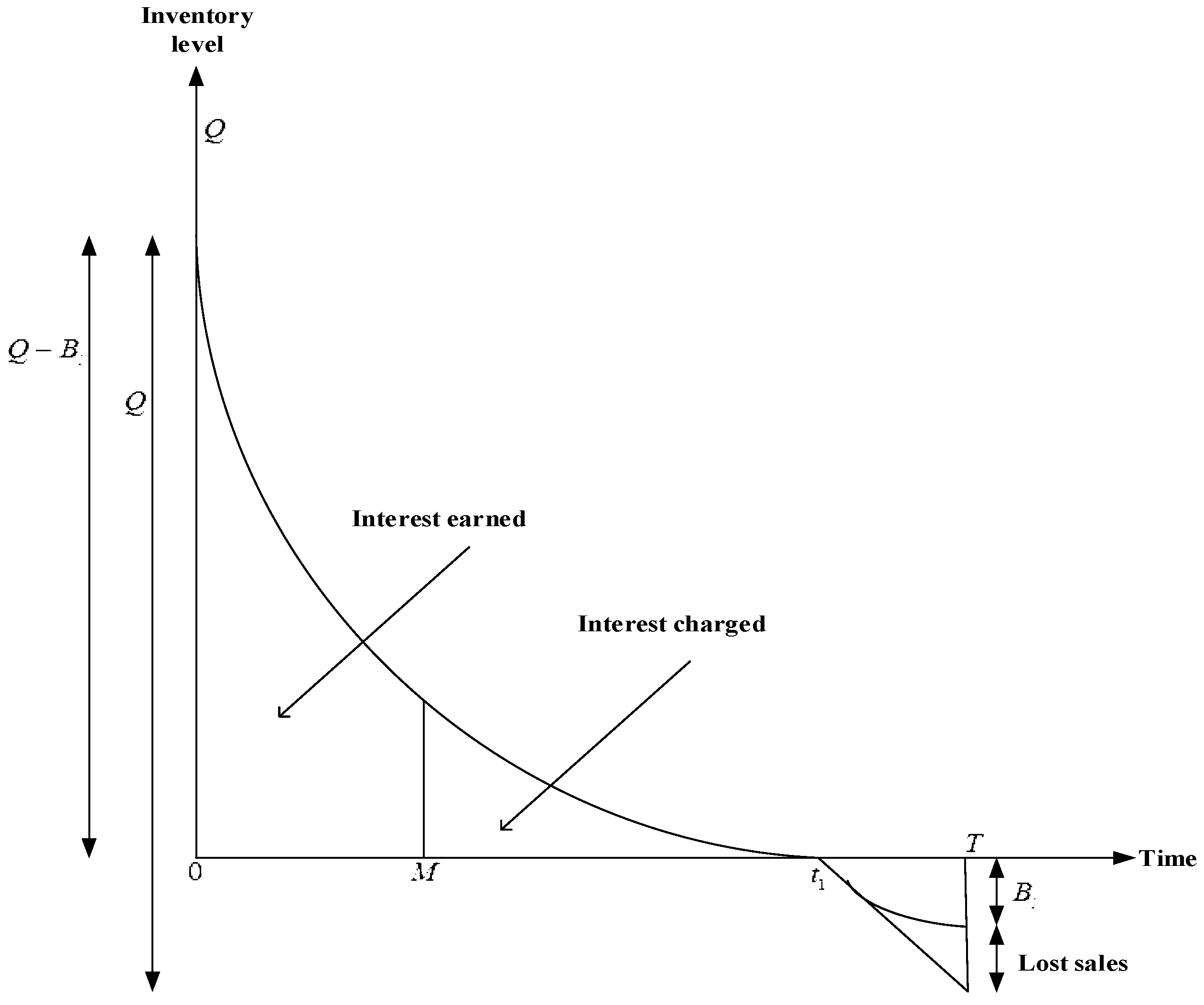
The mathematical model for perishable products with exponentially partially backlogged shortages under the demand based on the deterioration is presented in this section. Additionally, per cycle time the level of inventory drops according to both the deterioration rate and demand for the product. Furthermore, the graph of the level of inventory against cycle time T is represented in Figure 1.
Now, because of the deterioration-dependent rate of demand, the level of inventory decreases in time [ 0 , t 1 ] and the inventory level vanishes at a time t 1 . Thus, the level of inventory during the time [ 0 , t 1 ] can be obtained as
d I 1 ( t ) d t = θ I 1 ( t ) D ( θ ) ,           0 t t 1
Under the boundary condition I 1 ( t 1 ) = 0 , the stock level at any time t [ 0 , t 1 ] from Equation (5) can be obtained as
I 1 ( t ) = D 0 β θ θ [ e θ ( T t ) 1 ] ,                 0 t t 1
Next, at a time t = t 1 , the inventory level vanishes, resulting in shortages of the structure that increase exponentially e ς ( T t ) , ς > 0 with the T t wait time until the next shipment arrives in the system. Additionally, the maximum shortages level might be attained at the time t = T as indicated by B l . Therefore, the level of inventory during the interval [ t 1 , T ] can be evaluated as follows:
d I 2 ( t ) d t = D ( θ ) e ς ( T t ) ,           t 1 t T
As per the boundary condition I 2 ( t 1 ) = 0 , the level of stock at any time t [ t 1 , T ] from Equation (7) is:
I 2 ( t ) = D 0 β θ ς ( e ς ( T t ) e ς ( T t 1 ) )
Additionally, another boundary condition I 2 ( T ) = B l gives
B l = B l ( T ) = D 0 β θ ς ( 1 e ς ( T t 1 ) )
Since I 1 ( 0 ) = Q B l , as per the replenishment time T , the order quantity is obtained via Equations (6) and (9).
Q B l = D 0 β θ θ [ e θ T 1 ] Q = B l + D 0 β θ θ [ e θ T 1 ] Q = ( D 0 β θ ) ( ( 1 e ς ( T t 1 ) ) ς + ( e θ T 1 ) θ )
Next, the amount of sales that are lost at a time t [ t 1 , T ] is derived as:
N l ( t ) = t 1 t D ( θ ) ( 1 e ς ( T t ) ) d t ,         t 1 t T N l ( t ) = ( D 0 β θ ) ( ς ( t t 1 ) + e ς ( T t 1 ) e ς ( T t ) ) ς .
Now, in this model, a supplier provides goods to a retailer with allowable payment delay which is the trade credit policy. The interest received, interest charge, and total cost function are analyzed and also optimize the deterioration rate as follows in various circumstances:
Case (I):  ( 0 < M < t 1 )
During this situation, the credit phase arises before the inventory vanishes in the system which means a supplier allots a period of credit M to a retailer before a time t 1 . Throughout the time [ 0 , M ] , the retailer receives interest on the profit earned through sustaining shortages in the preceding cycle (see Figure 2).
Hence, the earned interest by a retailer can be estimated as:
I E 1 = S I e 0 M t D ( θ ) d t + S I e 0 M B l ( T ) d t I E 1 = S I e ( D 0 β θ ) M [ 1 2 M + ( 1 e ς ( T t 1 ) ) ς ]
The retailer earns interest throughout the interval [ 0 , M ] , but after the credit time M a retailer charges for the interest on unsold goods in the time period [ M , t 1 ] . Therefore, the interest charge of a retailer can be calculated as:
I C 1 = P I c M t 1 I 1 ( t ) d t I C 1 = P I c ( D 0 β θ θ ) ( e T θ t 1 θ + e M θ + T θ θ t 1 + M )
Case (II):  ( 0 < t 1 < M )
In this situation, the credit period occurs after the inventory vanishes in the system which means a supplier provides a credit period M to a retailer after a time t = t 1 . So, all the products received from the supplier were sold on credit by the retailer throughout the time [ 0 , M ] . Thus, the interest charged to a retailer was zero (i.e., I C 2 = 0 ) in the system. The retailer only receives interest on sold products throughout the time [ 0 , M ] and also earns interest on additional inventory throughout the interval [ t 1 , M ] (see Figure 3).
As an outcome, the earned interest by a retailer is calculated as:
I E 2 = S I e 0 t 1 t D ( θ ) d t + S I e 0 M B l ( T ) d t + S I e D ( θ ) ( M t 1 ) t 1 I E 2 = 1 2 S I e ( D 0 β θ ) t 1 2 + S I e ( 1 e ς ( T t 1 ) ) ( D 0 β θ ) M ς + S I e ( M t 1 ) ( D 0 β θ ) t 1
I C 2 = 0
Now, the total cost components per cycle time T are identified as:
  • Cost of ordering per order: O C = K
  • Cost of holding per unit per unit time: H C = [ h + h c ( 1 θ ) α ] 0 t 1 I 1 ( t ) d t = [ h + h c ( 1 θ ) α ] ( D 0 β θ ) ( e θ T e θ ( T t 1 ) t 1 θ ) θ 2
  • Cost of deterioration per cycle time T : D C = c p ( Q 0 t 1 D ( θ ) d t ) = c p ( D 0 β θ ) ( 1 e ς ( T a + T ) ς + e θ T θ 1 t 1 )
  • Cost of backlogging per unit: B C = c b t 1 T I 2 ( t ) d t = c b ( D 0 β θ ) ( e ς ( T t 1 ) ( ς T ς t 1 + 1 ) 1 ) ς 2
  • Cost of lost sales per cycle time T : LC = c 0 D ( θ ) t 1 T ( 1 e ς ( T t ) ) d t = c 0 ( D 0 β θ ) ( ς ( T t 1 ) + e ς ( T t 1 ) 1 ) ς
Hence, the total cost function per cycle time T of a retailer is stated as
T C i ( T , θ ) = 1 T ( O C + H C + D C + B C + L C + I C i I E i ) ;   i = 1 , 2 T C i ( T , θ ) = { T C 1 ( T , θ )           if         0 < M < t 1 < T T C 2 ( T , θ )           if         0 < t 1 < M < T
in which
T C 1 = 1 T ( K + ( h + h c ( 1 θ ) α ) ( D 0 β θ ) ( e θ ( T t 1 ) t 1 θ + e θ T ) θ 2 + c p ( D 0 β θ ) ( 1 e ς ( T a + T ) ς + e θ T θ 1 t 1 ) + c b ( D 0 β θ ) ( e ς ( T t 1 ) ( ς T ς t 1 + 1 ) 1 ) ς 2 + c 0 ( D 0 β θ ) ( ς ( T t 1 ) + e ς ( T t 1 ) 1 ) ς + P I c ( D 0 β θ θ ) ( e T θ t 1 θ + e M θ + T θ θ t 1 + M ) S I e ( D 0 β θ ) M ( 1 2 M + ( 1 e ς ( T t 1 ) ) ς ) ) T C 1 ( T , θ ) = 1 T ( K + ( D 0 β θ ) ( ( h + h c ( 1 θ ) α ) ( ( 1 + θ T + θ 2 T 2 2 ) a T θ e T a θ + T θ ) θ 2 c b ( e ς ( T a + T ) ( T ( 1 a ) ς + 1 ) 1 ) + ( 1 e ς ( T a + T ) ς ) ( c p S I e M c 0 ) + c p T ( 1 a + θ T 2 ) + c 0 T ( 1 a ) 1 2 S I e M 2 + P I c θ ( e T a θ + T θ + e M θ + T θ θ a T + M ) ) )
and
T C 2 = 1 T ( K + ( h + h c ( 1 θ ) α ) ( D 0 β θ ) ( e θ ( T t 1 ) t 1 θ + e θ T ) θ 2 + c p ( D 0 β θ ) ( 1 e ς ( T a + T ) ς + e θ T θ 1 t 1 ) + c b ( D 0 β θ ) ( e ς ( T t 1 ) ( ς T ς t 1 + 1 ) 1 ) ς 2 + c 0 ( D 0 β θ ) ( ς ( T t 1 ) + e ς ( T t 1 ) 1 ) ς S I e ( D 0 β θ ) ( 1 2 t 1 2 + M ( 1 e ς ( T t 1 ) ) ς + ( M t 1 ) t 1 ) ) T C 2 ( T , θ ) = 1 T ( K + ( D 0 β θ ) ( ( h + h c ( 1 θ ) α ) ( ( 1 + θ T + θ 2 T 2 2 ) a T θ e T a θ + T θ ) θ 2 c b ( e ς ( T a + T ) ( T ( 1 a ) ς + 1 ) 1 ) + ( 1 e ς ( T a + T ) ς ) ( c p S I e M c 0 ) + c p T ( 1 a + θ T 2 ) + c 0 T ( 1 a ) S I e a T ( M a T 2 ) ) )
After converting the exponential forms into the linear forms in the function of total cost, the first derivative with respect to T and θ for both cases can be evaluated as:
T C 1 ( T , θ ) T = 1 2 ( D 0 β θ ) ( 2 a 2 c b + h + h c ( 1 θ ) α 4 c b a + 2 c b + c p θ + M 2 I e S 2 T 2 ) K T 2 = 0
T C 2 ( T , θ ) T = 1 2 ( D 0 β θ ) ( I e S a 2 + 2 a 2 c b + h + h c ( 1 θ ) α + 4 c b a + 2 c b + c p θ ) K T 2 = 0
T C 1 ( T , θ ) θ = 1 2 T ( ( D 0 β θ ) ( 1 θ ) α 1 T 2 h c α 2 M I e S T β ( a 1 ) 2 T 2 β c b ( a 1 ) 2 + S I e β M 2 ( 1 θ ) α T 2 β h c 2 T 2 β c p θ + T 2 c p D 0 T 2 β h + 4 T β c p ( a 1 ) ) = 0
T C 2 ( T , θ ) θ = ( 1 2 ( 1 θ ) α 1 T α h c ( D 0 β θ ) 1 2 I e S T a 2 β T β c b ( a 1 ) 2 + M I e S β 1 2 ( 1 θ ) α T β h c T β c p θ 1 2 T β h + 1 2 T c p D 0 + 2 β c p ( a 1 ) ) = 0
Theorem 1: 
For any given θ defined in the interval ( 0 , 1 ) we have:
Case (I)  ( 0 < M < t 1 ) : the total cost T C 1 ( T , θ ) in Equation (19) is convex in T and achieves its global minimum with regard to
T 1 * = ( M 2 S I e ( D 0 β θ ) 2 K ) ( β θ D 0 ) ( 2 c b ( a 1 ) 2 + h c ( 1 θ ) α + c p θ + h )
the optimal order quantity
Q 1 * = ( a 2 ) ( β θ D 0 ) ( M 2 S I e ( β θ D 0 ) + 2 K ) ( 2 c b ( a 1 ) 2 + h c ( 1 θ ) α + c p θ + h )
and optimum minimum cost
T C 1 * = K ( β θ D 0 ) ( E 1 + h c ( 1 θ ) α + c p θ ) ( X 1 ( 2 c p h c ( 1 θ ) α + E 2 + 2 c p 2 θ ) + E 3 + M I e S c p θ + M I e S h c ( 1 θ ) α ) K ( E 1 + h c ( 1 θ ) α + c p θ ) ( β θ D 0 )
where X 1 = ( a 1 ) , E 1 = I e S a 2 + 2 c b ( a + 1 ) 2 + h , E 2 = 2 c p h + 2 I e S c p a 2 , and E 3 = 2 M I e S c b ( a + 1 ) 2 + 4 c p c b ( a 1 ) 3 + M I e 2 S 2 a 2 + M I e S h in Equation (25).
Case (II)  ( 0 < t 1 < M ) : the total cost T C 2 ( T , θ ) in Equation (20) is convex in T and achieves its global minimum with regard to
T 2 * = 2 K ( D 0 β θ ) ( I e S a 2 + 2 c b ( a + 1 ) 2 + h c ( 1 θ ) α + c p θ + h )
the optimal order quantity
Q 2 * = ( a 2 ) 2 K ( D 0 β θ ) ( I e S a 2 + 2 c b ( a + 1 ) 2 + h c ( 1 θ ) α + c p θ + h )
and the optimum minimum cost
T C 2 * = ( ( D 0 β θ ) X 1 E 4 ( ( β θ D 0 ) ( 2 K c p θ + 2 K ( 1 θ ) α h c + E 5 ) + X 1 2 ( 2 M 2 I e S D 0 2 c b 2 M 2 I e S β 2 θ 2 c b 4 M 2 I e S β θ D 0 c b ) + ( D 0 2 + β 2 θ 2 ) ( M 2 I e S h + M 2 I e S h c ( 1 θ ) α ) 2 M 2 I e S β c p θ 2 D 0 + M 2 I e S β 2 c p θ 3 2 M 2 I e S β θ D 0 h c ( 1 θ ) α + θ E 6 ( D 0 β θ ) ( 2 c b ( a 1 ) 2 + h + h c ( 1 θ ) α + c p θ ) ( M 2 S I e ( β θ D 0 ) + 2 K ) ) )
where X 1 = ( a 1 ) , E 4 = ( M I e S 2 c p ) , E 5 = 4 K a 2 c b + 4 K c b + 2 K h 8 a K c b , and E 6 = ( M 2 I e S c p D 0 2 2 M 2 I e S β h D 0 ) in Equation (28).
Proof: 
See Appendix A. □

Discussion on the Different α Values

The rate of deterioration θ = 1 γ 1 α is controlled by two factors which are fresh quality technology indicator γ and the deterioration rate preservation factor α . For the different farmed items, the rate of deterioration will not be the same under identical storage conditions and the same preservation effort due to their different natural perishability characteristics. If the ideal rate of deterioration is known, then the FQT for managing the deterioration rate can be obtained via Equation (2).
Now, the discussion on the different α values is explained below.
  • When α = 0 then 1 α becomes infinite which is not possible and the equation θ = 1 γ 1 α is not solvable. Therefore, α = 0 is not conceivable.
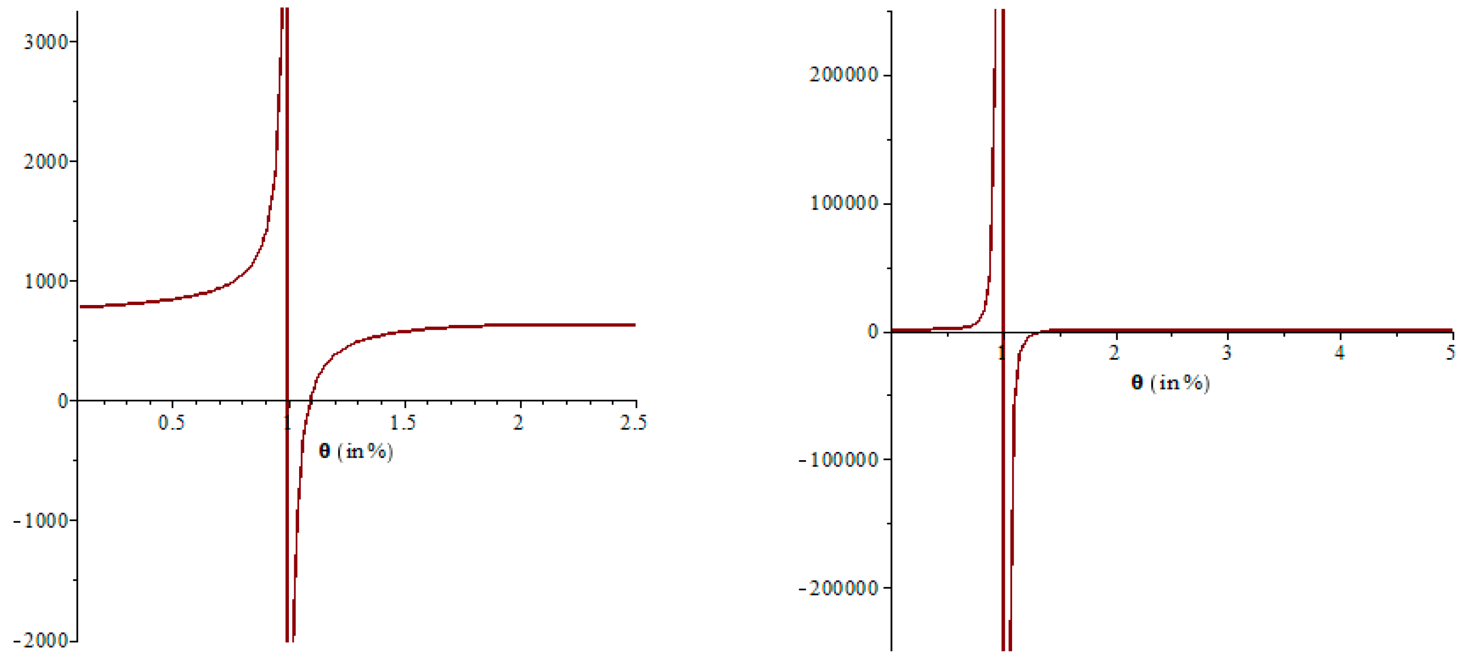
  • When α < 1 , then from Figure 4 it is observed that θ is not in the optimal range. Therefore, α < 1 is also not considered.
  • When 0 < α < 1 , it is noticed that deterioration rates for various items vary even when they are kept at the same freshness level. For various goods, the relationship coefficient between θ and α takes on different values. For illustration, with the same FQT and preservation cost, the rate of deterioration is different for oranges and grapes. Table 2 shows this, where α is as in Equation (1) and the FQT indicator γ is set to 0.4.
From Table 2, it is reflected that the higher the rate of α , the lower the rate of deterioration. If the value α is smaller than the product, then it is more susceptible to deterioration. As a result, 0 < α < 1 signifies situations during which perishable qualities are more significant than when α = 1 .
4.
When α 1 : from Figure 5 it is observed that the conceivable value α is greater or equal to 1. To verify that Equation (1) and other equations based on Equation (1) are reliable against changes in α values, the range α might be restricted to [ 1 , + ) . Therefore, in this model, the optimal rate of deterioration is discussed only for α = 1 and α > 1 . Furthermore, this portion concludes some managerial outcomes.

𝛼 = 1: Steps to make a decision

The second derivative of total cost function with respect to θ for Case (I) 0 < M < t 1 is
2 T C 1 ( T , θ ) θ 2 = T 2 ( ( D 0 β θ ) ( α 1 ) ( ( 1 θ ) α 2 α h c ) + 2 ( 1 θ ) α 1 α β h c 2 β c p )
It is difficult to identify the nature of the second derivative equation so when α = 1 the derivative becomes
2 T C 1 ( T , θ ) θ 2 = T β ( h c c p )
Additionally, it is the same for Case (II): 0 < t 1 < M
2 T C 2 ( T , θ ) θ 2 = T 2 ( ( D 0 β θ ) ( α 1 ) ( ( 1 θ ) α 2 α h c ) + 2 ( 1 θ ) α 1 α β h c 2 β c p )
and at α = 1 the second derivative becomes
2 T C 2 ( T , θ ) θ 2 = T β ( h c c p )
Now, Equations (30) and (32) allow for a simpler evaluation of the optimum solution.
Theorem 2: 
For the first case  ( 0 < M < t 1 )  when  α = 1  and  c p > h c  , the value of  θ  (noted as  θ 1 *  ) is
θ 1 * = D 0 2 β ( h + h c ) 2 ( c p h c ) + ( a 1 ) ( 2 c p M S I e ) T ( c p h c ) c b ( a 1 ) 2 ( c p h c ) + M 2 S I e 2 T 2 ( c p h c )
and the total cost function  T C 1 ( T , θ )  follows a saddle face, and for the case  ( 0 < t 1 < M )  when  α = 1  and  c p > h c  , the value of  θ  (noted as  θ 2 *  ) is
θ 2 * = D 0 2 β ( h + h c ) 2 ( c p h c ) c b ( a 1 ) 2 ( c p h c ) + 2 c p ( a 1 ) T ( c p h c ) S a 2 I e 2 ( c p h c ) + M S I e T ( c p h c )
and the total cost function  T C 2 ( T , θ )  follows a saddle face.
Proof: 
See Appendix B. □
Theorem 3: 
For the case  ( 0 < M < t 1 )  when  θ 1 * 1  , the optimum rate of deterioration tends to be 0, the equivalent optimum cycle time is  T 1 * = ( 2 K M 2 S I e D 0 ) D 0 ( 2 c b ( a 1 ) 2 + h c + h ) , and the optimum quantity of the order is  Q 1 * = ( a 2 ) D 0 ( M 2 S I e D 0 2 K ) ( 2 c b ( a 1 ) 2 + h c + h ) , and for the case  ( 0 < t 1 < M )  when  θ 2 * 1 , the optimum deterioration rate tends to be 0, the equivalent optimum cycle time is  T 2 * = 2 K D 0 ( I e S a 2 + 2 c b ( a + 1 ) 2 + h c + h ) , and the optimum order quantity is  Q 2 * = ( a 2 ) 2 K D 0 ( I e S a 2 + 2 c b ( a + 1 ) 2 + h c + h ) .
Proof: 
See Appendix C. □
Theorem 4: 
For the case  ( 0 < M < t 1 )  when  θ 1 * 0 , the optimal rate of deterioration tends to be 1, the equivalent optimal cycle time is  T 1 * = ( M 2 S I e ( D 0 β ) 2 K ) ( β D 0 ) ( 2 c b ( a 1 ) 2 + c p + h ) , and the optimum order quantity is defined as  Q 1 * = ( a 2 ) ( β D 0 ) ( M 2 S I e ( β D 0 ) + 2 K ) ( 2 c b ( a 1 ) 2 + c p + h ) , and for the case  ( 0 < t 1 < M )  when  θ 2 * 0 , the optimum rate of deterioration tends to be 1, an equivalent optimal cycle time is  T 2 * = 2 K ( D 0 β ) ( I e S a 2 + 2 c b ( a + 1 ) 2 + c p + h )  , and the optimum order quantity is  Q 2 * = ( a 2 ) 2 K ( D 0 β ) ( I e S a 2 + 2 c b ( a + 1 ) 2 + c p + h ) .
Proof: 
See Appendix D. □
The expressions of T i * and Q i * , i = 1 , 2 in Theorems 3 and 4 are similar to each other. The main difference between them is that in Theorem 3 there is no term for the deterioration cost and in Theorem 4 there is no term related to the marginal holding cost. Theorem 3 concludes that retailers should give full efforts to preserving the product to attain minimum deterioration and that this is applicable to high-value perishable products. Theorem 4 specifies that retailers should not try to preserve the product and that this is applicable to low-price products.
Now, for Theorem 5, values X's, Y's, Z's, and W's are shown in Table 3:
Theorem 5: 
For the case  ( 0 < M < t 1 )  when  0 < θ 1 * < 1 :
  • θ 1 *  and  Q 11 *  are not the global optimal solutions, where  Q 11 * = 1 2 ( 2 β T 2 X 2 1 X 3 2 β T 6 ( ( T X 1 Y 1 + T 2 X 3 Y 2 2 M 2 T 2 S β I e c b X 1 2 M 2 T 2 S β I e X 4 + Y 3 ) ( T X 1 Y 4 2 T 2 β c b X 1 2 + Y 5 T 2 β X 4 T 2 D 0 X 3 ) ) ) ( T X 1 Y 4 + 2 T 2 β c b X 1 2 + Y 5 T 2 β X 4 + T 2 D 0 X 3 )  is and the value of  Q 1 *  is at  θ = θ 1 * .
  • γ * 0  or  γ * 1
For case  ( 0 < t 1 < M )  when  0 < θ 2 * < 1 :
  • θ 2 *  and  Q 22 *  are not the global optimal solutions, where  Q 22 * = ( 2 β T X 2 K ( T Z 5 + Z 6 ) X 3 β T 2 ) T Z 5 + Z 6  is the value of  Q 2 *  at  θ = θ 2 * .
  • γ * 0  or  γ * 1
Proof: 
See Appendix E. □
Theorem 5 reflects the situation that falls in between the two extreme conditions. Based on their current management conditions, the enterprise can select the appropriate management technique. Theorem 5 concludes that when 0 < θ i * < 1   ; i = 1 , 2 there are some points where the overall cost attains its extreme at the specific value of Q   or   T . The total cost rises with the increasing rate of deterioration when 0 < θ i * < 1   ; i = 1 , 2 and the total cost decreases with the increasing rate of deterioration when θ > θ i * ; i = 1 , 2 . Therefore, for Case (I) except for when θ 1 * = D 0 2 β ( h + h c ) 2 ( c p h c ) + ( a 1 ) ( 2 c p M S I e ) T ( c p h c ) c b ( a 1 ) 2 ( c p h c ) + M 2 S I e 2 T 2 ( c p h c ) , at two different θ there should be two equivalent overall costs. For Case (II) except for the value of θ 2 * = D 0 2 β ( h + h c ) 2 ( c p h c ) c b ( a 1 ) 2 ( c p h c ) + 2 c p ( a 1 ) T ( c p h c ) S a 2 I e 2 ( c p h c ) + M S I e T ( c p h c ) , at two different θ there should be two equivalent overall costs. This suggests that under the same controlled-cost conditions, a retailer may sometimes decrease waste.
As a result, when α = 1 and c p > h c , the optimal deterioration rate that minimizes the total cost implies γ * { 1                                         θ 1   or   θ 2 1 1   or   0                     0 < θ 1   or   θ 2 < 1 0                                         θ 1   or   θ 2 0 .
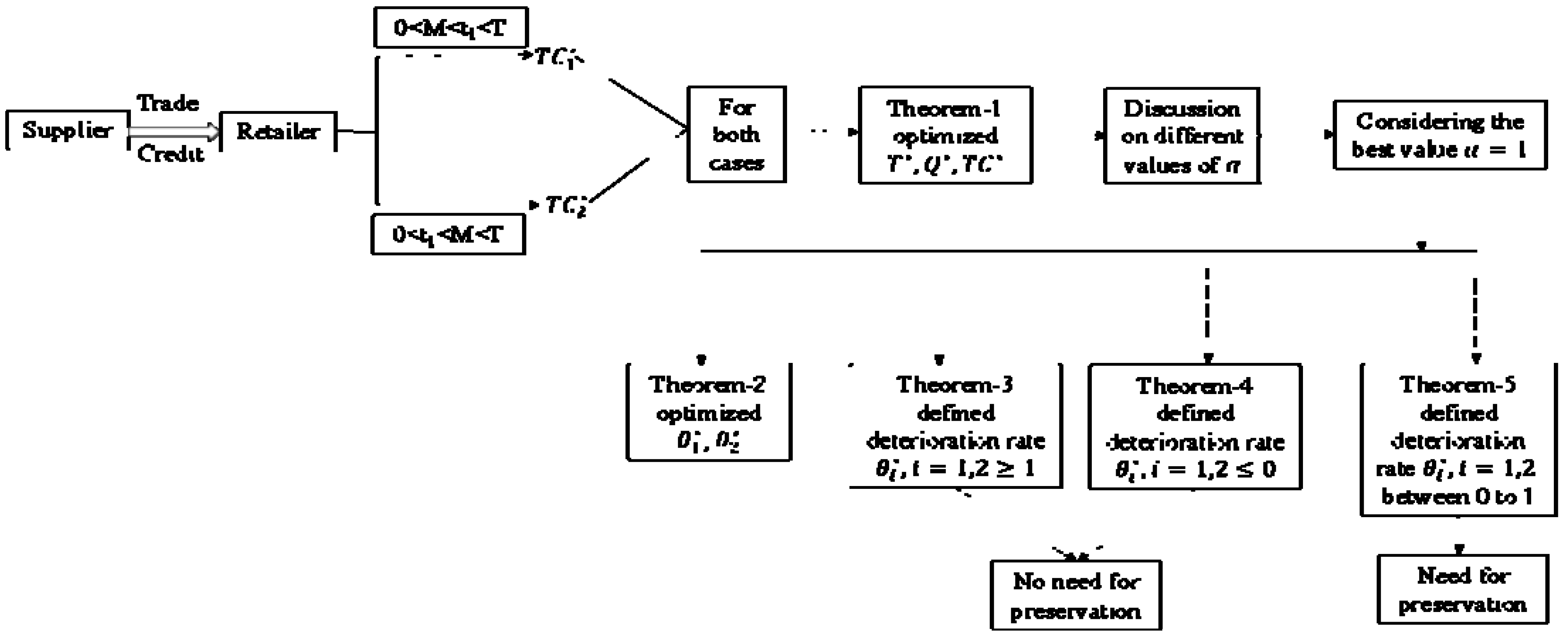
The previously stated results can help to improve a retailer’s ability to make relevant decisions. There are three steps to finding the decision.
First step: Correlate the cost of purchase c p with the maximum cost of holding h c which is relevant to keeping the product fresh.
Second step: If c p > h c , analyze the rate of θ i * for i = 1 , 2 . If θ i * 1 , the optimal value of the fresh quality technology indicator γ moves towards 1; if θ i * 0 , the optimal value of fresh quality technology indicator γ attempts 0; when 0 < θ i * < 1 , follow the third step.
Third step: This step consists of determining the overall cost when θ 0   or   θ 1 , and the lower value is selected by the retailer.
When the optimal FQT indicator attains 0 for both cases, the optimal cycle time is T 1 * = ( M 2 S I e ( D 0 β ) 2 K ) ( β D 0 ) ( 2 c b ( a 1 ) 2 + c p + h ) and T 2 * = 2 K ( D 0 β ) ( I e S a 2 + 2 c b ( a + 1 ) 2 + c p + h ) , and the optimal order quantities are Q 1 * = ( a 2 ) ( β D 0 ) ( M 2 S I e ( β D 0 ) + 2 K ) ( 2 c b ( a 1 ) 2 + c p + h ) and Q 2 * = ( a 2 ) 2 K ( D 0 β ) ( I e S a 2 + 2 c b ( a + 1 ) 2 + c p + h ) .
Additionally, the minimum total cost functions are T C 1 * = K ( β D 0 ) ( E 1 + c p ) ( X 1 ( E 2 + 2 c p 2 ) + E 3 ) K ( E 1 + c p ) ( β D 0 ) and T C 2 * = ( ( D 0 β ) X 1 E 4 ( ( β D 0 ) ( 2 K c p + E 5 ) + X 1 2 ( 2 M 2 I e S D 0 2 c b 2 M 2 I e S β 2 c b 4 M 2 I e S β D 0 c b ) + ( D 0 2 + β 2 ) ( M 2 I e S h ) + E 6 2 M 2 I e S β c p D 0 + M 2 I e S β 2 c p ( D 0 β ) ( 2 c b ( a 1 ) 2 + h + c p ) ( M 2 S I e ( β D 0 ) + 2 K ) ) ) .
Furthermore, when the optimal FQT indicator attains 1, for both cases the optimal order quantities are Q 1 * = ( a 2 ) D 0 ( M 2 S I e D 0 2 K ) ( 2 c b ( a 1 ) 2 + h c + h ) and Q 2 * = ( a 2 ) 2 K D 0 ( I e S a 2 + 2 c b ( a + 1 ) 2 + h c + h ) , the cycle times are T 1 * = ( 2 K M 2 S I e D 0 ) D 0 ( 2 c b ( a 1 ) 2 + h c + h ) , and T 2 * = 2 K D 0 ( I e S a 2 + 2 c b ( a + 1 ) 2 + h c + h ) , and the minimum total costs are T C 1 * = K D 0 ( E 1 + h c ) ( X 1 ( 2 c p h c + E 2 ) + E 3 + M I e S h 0 ) K ( E 1 + h c ) D 0 , and T C 2 * = ( ( D 0 ) X 1 E 4 ( ( D 0 ) ( 2 K h c + E 5 ) + X 1 2 ( 2 M 2 I e S D 0 2 c b ) + ( D 0 2 ) ( M 2 I e S h + M 2 I e S h c ) ( D 0 ) ( 2 c b ( a 1 ) 2 + h + h c ) ( M 2 S I e ( D 0 ) + 2 K ) ) ) .
As an outcome, Figure 6 shows the decision support system for the retailer.

5. Numerical Study and Sensitivity Analysis

5.1. Numerical Study

This model is applicable to perishable products such as fresh foods, dairy products, and some bakery items. To authenticate this model, two numerical examples are presented for both of the cases of trade credit policy. The comparable parameters’ values are extended from [2] to adapt the prototype.
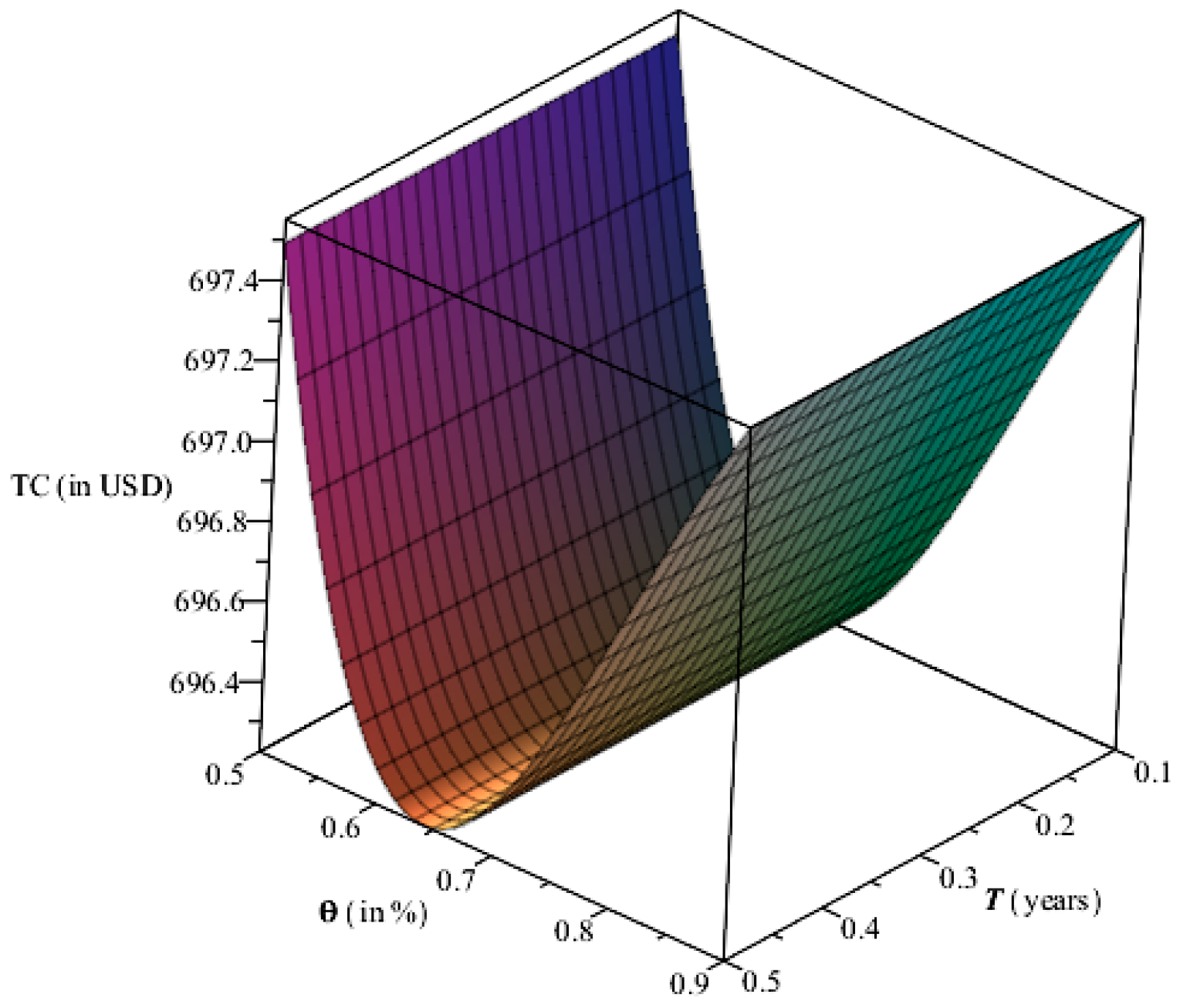
Illustration 1: For Case I  ( 0 < M < t 1 < T )  
Let  α = 4 ,   D 0 = 100   units / year ,   K = 40   USD / order ,   β = 15 ,   c b = 0.6   USD / unit   time ,   a = 0.8 ,   c p = 10 / units ,   ς = 0.7 ,   I e = 0.1 / USD / year ,   c 0 = 0.6   USD / unit   time ,   h = 10 / unit / unit   time ,   S = 30   USD / unit ,   h c = 8 / unit / unit   time ,   M = 0.1   years ,   I c = 0.12 / USD / year ,   P = 20   USD / unit .
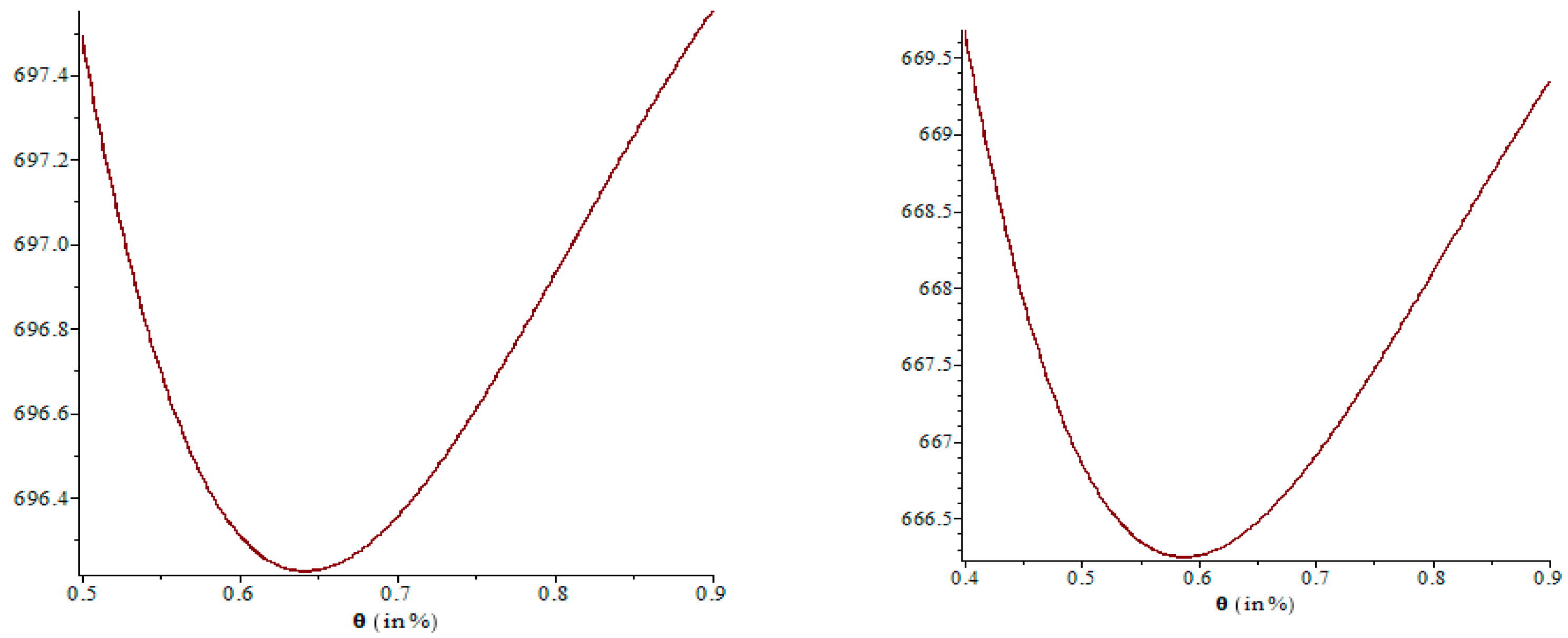
After solving this system, the optimum evaluates of decision variables are  T * = 0.219   years θ * = 0.64 , and total cost per cycle  T C 1 * ( T , θ ) = 696.23   USD ; the initial optimal quantity of order  Q * = 25.17   units  including the backorder quantity  B l * = 4   units . Additionally,  t 1 * = a T = 0.175   years , and  γ * = 0.016 .
The characteristic of convexity for the overall cost function T C 1 * ( T , θ ) is obtained in Figure 7.
Illustration 2: For Case II  ( 0 < t 1 < M < T )  
Use a similar set of statistics as with Illustration 1, with the exception of   M = 0.2   years .The optimal evaluates of decision variables are T * = 0.224   years  and  θ * = 0.58 , the total cost per cycle  T C 2 * ( T , θ ) = 666.24   USD , and the initial optimal quantity of order  Q * = 25.92   units  including backorder quantity  B l * = 4   units . Additionally,  t 1 * = a T = 0.179   years , and  γ * = 0.028 .
The convexity tendency of the overall cost function  T C 2 * ( T , θ )  is determined in Figure 8.

5.2. Sensitivity Analysis

In this section, sensitivity analysis is performed on Illustration 2 and shows a variation in decision variables by varying parameters of inventory values up to - 20 % ,   - 10 % ,   10 % ,   and   20 % .
The following observations are obtained from Table 4:
  • When the rate of deterioration preservation factor ( α ) increases, the FQT indicator ( γ ) , cycle time ( T ) , quantity of order ( Q ) , and the time considered for inventory level to drop to zero ( t 1 ) increase slowly while the deterioration rate ( θ ) decreases slowly. However, total cost ( T C ) decreases gradually.
  • There is a negative effect of fixed demand rate ( D 0 ) on total cost ( T C ) and FQT indicator ( γ ) . They all are increased rapidly. Further, order quantity ( Q ) increases slowly, and cycle time ( T ) , deterioration rate ( θ ) , and time considered for inventory level to drop to zero ( t 1 ) decrease slowly.
  • If ordering cost ( K ) increases, the deterioration rate ( θ ) decreases slowly while order quantity ( Q ) and time considered for inventory level to drop to zero ( t 1 ) increase slowly. However, total cost ( T C ) , FQT indicator ( γ ) , and cycle time ( T ) increase rapidly.
  • Change in the parameter’s sales price ( S ) and interest earned ( I e ) , total cost ( T C ) , the time considered for inventory level to drop to zero ( t 1 ) , cycle time ( T ) , order quantity ( Q ) , and FQT indicator ( γ ) decrease slowly. However, there are no changes in the rate of deterioration ( θ ) .
  • As the demand-on-quantity variable ( β ) changes, cycle time ( T ) , total cost ( T C ) , order quantity ( Q ) , and the time considered for inventory level to drop to zero ( t 1 ) decrease slowly, whereas the FQT indicator ( γ ) decreases rapidly and the deterioration rate ( θ ) increases rapidly.
  • The FQT indicator ( γ ) increases slowly and total cost ( T C ) decreases rapidly. Further, cycle time ( T ) , order quantity ( Q ) , the time considered for inventory level to drop to zero ( t 1 ) , and deterioration rate ( θ ) decrease slowly whenever the upstream trade credit period ( M ) changes.
  • As the holding parameter ( h ) increases, quantity of order ( Q ) decreases slowly and total cost ( T C ) decreases rapidly. On the other hand, cycle time ( T ) , the time considered for the stock level to drop to zero ( t 1 ) , and FQT indicator ( γ ) decrease rapidly and the rate of deterioration ( θ ) increases slowly.
  • As the cost of procurement ( c p ) varies, the deterioration rate ( θ ) increases slowly, while cycle time ( T ) , order quantity ( Q ) , and time considered for inventory level to drop to zero ( t 1 ) decrease slowly. Furthermore, total cost ( T C ) increases rapidly and the FQT indicator ( γ ) increases slowly; after that, it increases rapidly.
  • The cycle time ( T ) and time considered for level of inventory to drop to zero ( t 1 ) decrease slowly, the total cost ( T C ) increases rapidly, and then both become constant. However, order quantity ( Q ) decreases slowly, the deterioration rate ( θ ) increases slowly, and FQT indicator ( γ ) decreases rapidly when the maximum cost of holding parameter ( h c ) fluctuates.

5.3. Managerial Implications

  • A retailer should take a long credit period from the supplier to receive more benefits since the credit period significantly reduces the total cost per cycle time rapidly while the cycle time drops slowly.
  • Based on Theorem 3, a retailer should not invest in the preservation factor because the rate of deterioration is θ i 1 ; i = 1 , 2 which implies that the product fully deteriorates. So, there is no need to preserve and increase the total cost. For example, if all of the tomatoes, lemons, bread, flowers, and other perishable items fully deteriorate then the retailer should not invest to sustain that kind of product.
  • According to Theorem 4, if θ i 1 ; i = 1 , 2 then the retailer should not invest in preservation because the product is non-deteriorating. For example, if dry inventory, coffee powder, tea powder, etc., have zero deterioration rate then the retailer should not invest in the preservation factor to raise the cost.
  • According to Theorem 5, if the range of deterioration is 0 < θ i < 1 ; i = 1 , 2 then the retailer should invest in the preservation factor to preserve the perishable product and fulfill the demand of consumers. Dairy products, cooked leftovers, vegetables, fruits, and so on need a preservation and temperature environment according to their freshness. So, if the product is not fully deteriorated or non-deteriorating then the retailer should invest in the preservation factor because the demand is quality-dependent on the perishable product.
  • As Table 4 shows, the retailer should decrease the cost of holding parameter, reduce the ordering cost, focus on the quality of the perishable product, and adjust the sales price to generate more revenue and less expenditure.
  • If the rate of deterioration is low and demand is high, the retailer should buy additional inventory before the shortages occur. If the flowers are fresh, retailers will buy them, and demand will rise gradually. Therefore, before all of the flowers are sold, the retailer should order more flowers.
  • To achieve the optimal rate of deterioration, the value of the rate of the deterioration preservation factor α must be restricted [ 1 , ) . If the value of the rate of the deterioration preservation factor is less than 1, the optimal deterioration rate increases, implying a rise in the overall cost of a retailer. (See Table 2).

6. Conclusions

This study is inspired by a farmed product deterioration problem faced by a supplier selling vegetables or fresh fruits to a retailer, in which retailers are more willing to purchase at a given fixed price for better quality, less deteriorated, and more storable perishable items. This study is premised on prior research on perishable inventory control by investigating deterioration rate as a decision parameter and its consequences for perishable quality control indicators, associated customer demands, and a variable operational cost. In addition, this article assumes that demand is influenced by quality deterioration over a certain period. This work also assumes that the rate of deterioration can be controlled using FQT and effort as cost factors. In addition, the supplier offers its retailer a mutually acceptable trade credit. This advantages both the retailer and the supplier. Additionally, shortages are allowed. Furthermore, considering controlled deterioration/freshness-dependent demand, product quality indication, and manageable DR to analyze its dynamic behavior with several parameters including trade credit under allowable partially backlogged shortages, this EOQ model is a theoretical extension and an example of innovation with practical interpretations and implementations. This study has analytically analyzed this situation and conducted sensitivity analysis to develop managerial consequences.
Finally, this research concludes that the retailer should invest in the preservation factor when the rate of deterioration of the perishable product is between 0 and 1. If the rate of deterioration is 0, then the product is non-deteriorating and the retailer does not need to invest in the FQT indicator. Similarly, for the deterioration rate of 1 whereby the product already deteriorates, there is no need to spend on preservation. The value of the deterioration rate preservation factor must be in the interval of [ 1 , ) to obtain the optimum value of the deterioration rate as proved in the model. The retailer should order the inventory before the shortages occur in the system and the retailer should use the trade credit policy to minimize the total cost and earn more profit per cycle time. In addition, this model includes the correlation between the fresh quality indicator and the deterioration rate.
This approach is used in all areas that deal with the deterioration and quality of perishable goods, for example, fresh food items, frozen food items, fresh flowers, dairy products, seafood, cooked foods, fresh vegetables and fruits, etc., but this inventory model is derived under the following limitations:
  • This model discussed the relation between the fresh quality technology (FQT) indicator and controllable rate of deterioration. However, preservation technology was not applied to reduce the rate of deterioration. Additionally, the fluctuating rate of deterioration and the functional relationship between the rate of deterioration and the quality indicator are not considered in this model.
  • The proposed inventory model is developed with deterioration-dependent demand. This can be expanded for different kinds of demand such as fuzzy demand as shown in [43], freshness-dependent demand as discussed in [44], etc.
  • This study allows for a one-layered trade credit policy and partially backlogged shortages. In spite of this, one can consider a two-layered trade credit policy and fully backlogged shortages as shown in [45].

Author Contributions

Conceptualization, M.Y.J. and H.A.P.; methodology, A.B.; software, H.A.P.; resources, M.S.A.; writing—original draft preparation, A.B.; writing—review and editing, U.C.; supervision, M.Y.J.; funding acquisition, M.S.A. and M.A. All authors have read and agreed to the published version of the manuscript.

Funding

This research was funded by Deanship of Scientific Research at King Khalid University (KKU): R.G.P.1/349/43.

Data Availability Statement

Not applicable.

Acknowledgments

The authors extend their appreciation to the Deanship of Scientific Research at King Khalid University (KKU) for funding this research project (Number R.G.P.1/349/43).

Conflicts of Interest

The authors declare no conflict of interest.

Nomenclature

This article consists of the following notation and assumptions to emerge a mathematical model of a proposed problem.
Parameters
K Ordering cost; (in USD/order)
P Purchasing cost; (in USD/unit)
h Holding cost; (in USD/unit/unit time)
h c The maximum cost of holding including preservation; (in USD/unit/unit time)
h θ The controllable marginal cost of holding including preservation; 0 < h θ < h c
γ Indicator of fresh quality technology; 0 < γ < 1
α Rate of deterioration with the factor of preservation; α > 0
D 0 Fixed rate of demand
β The factor of quality-related variation in demand; β > 0
D Total demand; (in years)
M Upstream trade credit; (in years)
I e Earned interest of a retailer; (in %/year)
I c Charged interest of a retailer; (in %/year)
ς Backlogging factor; ς > 0
B l The total volume of backlog based on demand; (in units)
Q Retailer’s quantity of order per cycle time; (in units)
c p Procurement cost; (in USD/unit)
c b Backlogging cost; (in USD/unit time)
c 0 Cost of unit opportunity due to lost sale; (in USD/unit time)
S The product’s sales price; (in USD/unit)
Decision variables
T Cycle time; (in years)
θ Deterioration rate; 0 < θ < 1
Functions
t 1 ( T ) = a T ; time considered for a stock level to drop to zero, where a > 0 (in years)
I 1 ( t ) The on-hand stock level at a time t ; 0 t t 1 (units)
I 2 ( t ) Backlogged level of stock at a time t ; t 1 t T (units)
N l ( t ) Lost sales number at a time t ; (units)
T C i ( T , θ ) The function of total profit per unit time t for i = 1 , 2 ; (in USD)

Appendix A. Proof of Theorem 1

For Case (I) ( 0 < M < t 1 ) , for any given θ ( 0 , 1 ) , the optimal cycle time T 1 * = ( M 2 S I e ( D 0 β θ ) 2 K ) ( β θ D 0 ) ( 2 c b ( a 1 ) 2 + h c ( 1 θ ) α + c p θ + h ) can be derived by solving Equation (19). After that, for finding the optimal order quantity, replace the value of T with T 1 * in Equation (10). So, the optimal order quantity is derived as Q 1 * = ( a 2 ) ( β θ D 0 ) ( M 2 S I e ( β θ D 0 ) + 2 K ) ( 2 c b ( a 1 ) 2 + h c ( 1 θ ) α + c p θ + h ) . Additionally, check the second-order derivative 2 T C 1 ( T , θ ) T 2 = M 2 S I e ( β θ D 0 ) + 2 K T 3 > 0 which indicates that the total cost function achieves its global minimum; it can be derived after substituting T 1 * back to Equation (17). Hence, the optimum total cost function is specified as
T C 1 * = K ( β θ D 0 ) ( E 1 + h c ( 1 θ ) α + c p θ ) ( X 1 ( 2 c p h c ( 1 θ ) α + E 2 + 2 c p 2 θ ) + E 3 + M I e S c p θ + M I e S h c ( 1 θ ) α ) K ( E 1 + h c ( 1 θ ) α + c p θ ) ( β θ D 0 )
where X 1 = ( a 1 ) , E 1 = I e S a 2 + 2 c b ( a + 1 ) 2 + h , E 2 = 2 c p h + 2 I e S c p a 2 , and E 3 = 2 M I e S c b ( a + 1 ) 2 + 4 c p c b ( a 1 ) 3 + M I e 2 S 2 a 2 + M I e S h
For Case (II) ( 0 < t 1 < M ) :
The proof of Case (II) is parallel to Case (I) and the determined optimum value of cycle time is T 2 * = 2 K ( D 0 β θ ) ( I e S a 2 + 2 c b ( a + 1 ) 2 + h c ( 1 θ ) α + c p θ + h ) , order quantity is Q 2 * = ( a 2 ) 2 K ( D 0 β θ ) ( I e S a 2 + 2 c b ( a + 1 ) 2 + h c ( 1 θ ) α + c p θ + h ) , and the total cost is defined as
T C 2 * = ( ( D 0 β θ ) X 1 E 4 ( ( β θ D 0 ) ( 2 K c p θ + 2 K ( 1 θ ) α h c + E 5 ) + X 1 2 ( 2 M 2 I e S D 0 2 c b 2 M 2 I e S β 2 θ 2 c b 4 M 2 I e S β θ D 0 c b ) + ( D 0 2 + β 2 θ 2 ) ( M 2 I e S h + M 2 I e S h c ( 1 θ ) α ) 2 M 2 I e S β c p θ 2 D 0 + M 2 I e S β 2 c p θ 3 2 M 2 I e S β θ D 0 h c ( 1 θ ) α + θ E 6 ( D 0 β θ ) ( 2 c b ( a 1 ) 2 + h + h c ( 1 θ ) α + c p θ ) ( M 2 S I e ( β θ D 0 ) + 2 K ) ) )
where X 1 = ( a 1 ) , E 4 = ( M I e S 2 c p ) , E 5 = 4 K a 2 c b + 4 K c b + 2 K h 8 a K c b , and E 6 = ( M 2 I e S c p D 0 2 2 M 2 I e S β h D 0 ) .

Appendix B. Proof of Theorem 2

For Case (I) ( 0 < M < t 1 ) :
When α = 1 and c p > h c , the value of θ 1 * can be calculated using Equation (21):
θ 1 * = D 0 2 β ( h + h c ) 2 ( c p h c ) + ( a 1 ) ( 2 c p M S I e ) T ( c p h c ) c b ( a 1 ) 2 ( c p h c ) + M 2 S I e 2 T 2 ( c p h c )
Additionally, from the second derivative 2 T C 1 ( T , θ ) θ 2 = T β ( c p h c ) < 0 , it is observed that the function of the total cost has a saddle face. The optimum deterioration rate can easily be estimated to be 0 or 1.
For Case (II) ( 0 < t 1 < M ) the proof is parallel to Case (I).

Appendix C. Proof of Theorem 3

For Case (I) ( 0 < M < t 1 ) :
Here, θ 1 * 1 which is above the deterioration rate’s normal range. Hence, the optimum solution cannot be reached with θ 1 * , and it should be calculated using alternative methods. The overall cost function’s first partial derivative with respect to θ when α = 1 is derived as T C 1 ( T , θ ) θ = 1 2 ( 2 M S a β I e + 2 M S β I e + 4 T a β c b 2 T β θ c p + T β θ h c T β h 2 T β c b T β h c + T c p D 0 T D 0 h c + 4 a β c p 4 β c p ) .
The first derivative of a function of total cost T C 1 ( T , θ ) θ is a linear function of θ . As an outcome, if a line 1 2 ( 2 M S a β I e + 2 M S β I e + 4 T a β c b 2 T β θ c p + T β θ h c T β h 2 T β c b T β h c + T c p D 0 T D 0 h c + 4 a β c p 4 β c p ) has a positive slope, then the optimal value of deterioration rate θ * 0 , which directs γ * 1 . Otherwise, the optimal value is at θ * 1 which indicates that γ * 0 as θ 1 * 1 , i.e., D 0 2 β ( h + h c ) 2 ( c p h c ) + ( a 1 ) ( 2 c p M S I e ) T ( c p h c ) c b ( a 1 ) 2 ( c p h c ) + M 2 S I e 2 T 2 ( c p h c ) 1 . From this equation, one can see ( ( c p h c ) T 2 D 0 + 4 T β c p ( a 1 ) T 2 β ( h + h c ) 2 T 2 β c b ( a 1 ) 2 2 M S T β I e ( a 1 ) + M 2 S β I e ) 2 T 2 β ( c p h c ) . In Equation (21), T is replaced by T * with c p > h c and it is observed that T C 1 ( T * , θ ) θ > 1 2 ( 2 M S a β I e + 2 M S β I e + 4 T * a β c b 2 T * β θ c p + T * β θ h c T * β h 2 T * β c b T * β h c + T * c p D 0 T * D 0 h c + 4 a β c p 4 β c p ) 0 which denotes that the slope of a line 1 2 ( 2 M S a β I e + 2 M S β I e + 4 T * a β c b 2 T * β θ c p + T * β θ h c T * β h 2 T * β c b T * β h c + T * c p D 0 T * D 0 h c + 4 a β c p 4 β c p ) is always positive. As a result, as θ and its related optimal fixed quantity of order increase the total cost increases. In this case, θ * 0 . If the retailer wants to keep the product fresh, then they must attempt to preserve as much as possible. So, for this case of h θ h c , the fresh quality technology indicator γ * 1 .
From Theorem 1 Case (I), the optimal cycle time and order quantity, respectively, are T 1 * = ( 2 K M 2 S I e D 0 ) D 0 ( 2 c b ( a 1 ) 2 + h c + h ) and Q 1 * = ( a 2 ) D 0 ( M 2 S I e D 0 2 K ) ( 2 c b ( a 1 ) 2 + h c + h ) .
For Case (II) ( 0 < t 1 < M ) , the proof is analogous to Case (I).
The result is that to keep the product fresh, a retailer must perform all that is necessary to preserve it. For this case of h θ h c , a fresh quality technology indicator γ * 1 .
The optimum values of cycle time and quantity of the order from Theorem 1 Case (II) are T 2 * = 2 K D 0 ( I e S a 2 + 2 c b ( a + 1 ) 2 + h c + h ) and Q 2 * = ( a 2 ) 2 K D 0 ( I e S a 2 + 2 c b ( a + 1 ) 2 + h c + h ) .

Appendix D. Proof of Theorem 4

For Case (I) ( 0 < M < t 1 ) :
Here, the rate of deterioration is θ 1 * 0 ; from Equation (33), one can obtain ( ( c p h c ) T 2 D 0 + 4 T β c p ( a 1 ) T 2 β ( h + h c ) 2 T 2 β c b ( a 1 ) 2 2 M S T β I e ( a 1 ) + M 2 S β I e ) 0 . The total cost function’s first derivative with respect to θ after the replaced value of T with T * is T C 1 ( T * , θ ) θ < 1 2 ( 2 M S a β I e + 2 M S β I e + 4 T * a β c b 2 T * β θ c p + T * β θ h c T * β h 2 T * β c b T * β h c + T * c p D 0 T * D 0 h c + 4 a β c p 4 β c p ) 0 which indicates that the slope is always negative. As a result, as θ and its related optimal fixed quantity of order decrease, the overall cost decreases. In this case, θ * 1 . Therefore, the most effective way for a retailer to reduce the overall cost is to do nothing to keep the inventory fresh. So, for this case of h θ 0 , the indicator of fresh quality technology is γ * 0 . According to Theorem 1 Case (I), the equivalent optimum cycle time and the order quantity are T 1 * = ( M 2 S I e ( D 0 β ) 2 K ) ( β D 0 ) ( 2 c b ( a 1 ) 2 + c p + h ) and Q 1 * = ( a 2 ) ( β D 0 ) ( M 2 S I e ( β D 0 ) + 2 K ) ( 2 c b ( a 1 ) 2 + c p + h ) .
For Case (II) ( 0 < t 1 < M ) the proof is similar to Case (I).
As a result, the most effective way for a retailer to reduce the overall cost is to do nothing to keep the inventory fresh. So, for this case of h θ 0 , an indicator of fresh quality technology is γ * 0 . From Theorem 1 Case (II), the optimum cycle time is T 2 * = 2 K ( D 0 β ) ( I e S a 2 + 2 c b ( a + 1 ) 2 + c p + h ) and the optimum order quantity is Q 2 * = ( a 2 ) 2 K ( D 0 β ) ( I e S a 2 + 2 c b ( a + 1 ) 2 + c p + h ) .

Appendix E. Proof of Theorem 5

For Case (I) ( 0 < M < t 1 ) :
When 0 < θ 1 * < 1 , the necessary condition for the lowest overall cost is θ 1 * = D 0 2 β ( h c + h ) 2 ( c p h c ) + ( a 1 ) ( 2 c p M S I e ) T ( c p h c ) c b ( a 1 ) 2 ( c p h c ) + M 2 S I e 2 T 2 ( c p h c ) and Q 11 * = 1 2 ( 2 β T 2 X 2 1 X 3 2 β T 6 ( ( T X 1 Y 1 + T 2 X 3 Y 2 2 M 2 T 2 S β I e c b X 1 2 M 2 T 2 S β I e X 4 + Y 3 ) ( T X 1 Y 4 2 T 2 β c b X 1 2 + Y 5 T 2 β X 4 T 2 D 0 X 3 ) ) ) ( T X 1 Y 4 + 2 T 2 β c b X 1 2 + Y 5 T 2 β X 4 + T 2 D 0 X 3 )
( T 11 * = ( 2 β T 4 X 3 1 X 3 2 β T 6 ( ( T X 1 Y 1 + T 2 X 3 Y 2 2 M 2 T 2 S β I e c b X 1 2 M 2 T 2 S β I e X 4 + Y 3 ) ( T X 1 Y 4 2 T 2 β c b X 1 2 + Y 5 T 2 β X 4 T 2 D 0 X 3 ) ( T X 1 Y 4 + 2 T 2 β c b X 1 2 + Y 5 T 2 β X 4 + T 2 D 0 X 3 ) ) ) 4 X 1 2 T 2 ( Y 10 T 2 Y 6 ) + 4 T X 1 Y 7 2 X 3 T 4 Y 8 + T 4 Y 9 + Y 5 2 )
( Q 11 * and T 11 * are the values of order quantity and cycle time at θ = θ 1 * ).
Now, at this point ( θ 1 * , Q 11 * / T 11 * ) , the hessian matrix for the local minimum H 1 = [ 2 T C 1 ( T , θ ) θ 2 2 T C 1 ( T , θ ) θ T 2 T C 1 ( T , θ ) T θ 2 T C 1 ( T , θ ) T 2 ] is positive and satisfies the following conditions: 2 T C 1 ( T , θ ) θ 2 = T 11 * β ( c p h c ) < 0 , 2 T C 1 ( T , θ ) T 2 = 1 T 11 * 3 ( M 2 S I e ( β θ D 0 ) + 2 K ) > 0 . Additionally, the value of the hessian matrix is 1 4 T 4 ( ( 4 T 4 β 2 c b 2 X 1 4 ) + 4 X 1 2 ( M 2 S T 2 β 2 I e c b + 2 β 2 T 4 c p θ c b 2 T 4 β 2 θ c b h c + T 4 Z 1 ) + X 3 ( 8 M 2 T 2 S β 2 θ I e + 4 β 2 T 2 c p θ 2 + T 2 Z 2 2 T 4 β D 0 h c ) + T 4 X 3 2 ( D 0 2 4 β θ D 0 ) + X 4 ( 4 T 4 β 2 c p θ + 2 M 2 S T 2 β 2 I e ) + T 4 β 2 X 5 + 4 T 4 β 2 θ h c 2 ( θ 1 ) 2 T 4 Z 3 4 T 4 β 2 h θ h c + 2 T 4 Z 4 + Y 5 ) < 0 .
Therefore, ( θ 1 * , Q 11 * / T 11 * ) becomes a saddle point.
From the above proof, T * can be obtained by the fixed value of θ * ; θ * cannot equal θ 1 *  because 2 T C 1 ( T , θ ) θ 2 < 0 . θ 1 * is the point of maximum cost; the lower the total cost, the greater the distance from this point, and the best deterioration rate should be closer to 0 or 1 which indicates that γ * 1 or γ * 0 .
For Case (II) ( 0 < t 1 < M ) , the proof is similar to Case (I).
The optimum values of cycle time and order quantity when θ = θ 2 * are T 22 * = ( 2 β T 2 X 3 2 X 3 β T 2 K ( T Z 5 + Z 6 ) ( T Z 5 + Z 6 ) ) S 2 T 2 a 4 β 2 I e 2 4 S T 2 β 2 I e c b ( a X 1 ) 2 4 T 2 β 2 c b 2 X 1 4 + T 2 ( X 3 Z 8 Z 9 + X 4 Z 7 ) + Z 10 and Q 22 * = ( 2 β T X 2 K ( T Z 5 + Z 6 ) X 3 β T 2 ) T Z 5 + Z 6 . In this case, ( θ 2 * , Q 22 * / T 22 * ) becomes a saddle point.
Here, θ 2 * is the point of maximum cost; the lower the total cost, the greater the distance from this point, and the optimal deterioration rate should be closer to 0 or 1 which indicates that γ * 1 or γ * 0 .

References

  1. Cai, X.; Chen, J.; Xiao, Y.; Xu, X. Optimization and coordination of fresh product supply chains with freshness-keeping effort. Prod. Oper. Manag. 2010, 19, 261–278. [Google Scholar] [CrossRef]
  2. Yang, Y.; Chi, H.; Zhou, W.; Fan, T.; Piramuthu, S. Deterioration control decision support for perishable inventory management. Decis. Support Syst. 2020, 134, 113308. [Google Scholar] [CrossRef]
  3. Xu, G.; Wu, H.; Liu, Y.; Wu, C.-H.; Tsai, S.-B. A Research on Fresh-Keeping Strategies for Fresh Agricultural Products from the Perspective of Green Transportation. Discret. Dyn. Nat. Soc. 2020, 2020, 1307170. [Google Scholar] [CrossRef]
  4. Tu, Y.J.; Zhou, W.; Piramuthu, S. A novel means to address RFID tag/item separation in supply chains. Decis. Support Syst. 2018, 115, 13–23. [Google Scholar] [CrossRef]
  5. Bakker, M.; Riezebos, J.; Teunter, R.H. Review of inventory systems with deterioration since 2001. Eur. J. Oper. Res. 2012, 221, 275–284. [Google Scholar] [CrossRef]
  6. Cárdenas-Barrón, L.E.; Shaikh, A.A.; Tiwari, S.; Treviño-Garza, G. An EOQ inventory model with nonlinear stock dependent holding cost, nonlinear stock dependent demand and trade credit. Comput. Ind. Eng. 2018, 139, 105557. [Google Scholar] [CrossRef]
  7. Shaikh, A.A.; Das, S.C.; Bhunia, A.K.; Sarkar, B. Decision support system for customers during availability of trade credit financing with different pricing situations. RAIRO-Oper. Res. 2021, 55, 1043–1061. [Google Scholar] [CrossRef]
  8. Shaikh, A.A. A two-warehouse inventory model for deteriorating items with variable demand under alternative trade credit policy. Int. J. Logist. Syst. Manag. 2017, 27, 40–61. [Google Scholar] [CrossRef]
  9. Jaggi, C.K.; Gautam, P.; Khanna, A. Quality, Inventory decisions for imperfect quality deteriorating items with exponential declining demand under trade credit and partially backlogged shortages. In Quality, IT and Business Operations, Springer Proceedings in Business and Economics; Kapur, P., Kumar, U., Verma, A., Eds.; Springer: Berlin/Heidelberg, Germany, 2018; Chapter 18; pp. 213–229. [Google Scholar] [CrossRef]
  10. Tripathi, R.P. Innovation of economic order quantity (EOQ) model for deteriorating items with time-linked quadratic demand under non-decreasing shortages. Int. J. Appl. Comput. Math. 2019, 5, 123. [Google Scholar] [CrossRef]
  11. Namdeo, A.; Khedlekar, U.K.; Singh, P. Discount pricing policy for deteriorating items under preservation technology cost and shortages. J. Manag. Anal. 2020, 7, 1–23. [Google Scholar] [CrossRef]
  12. Shaikh, A.A.; Panda, G.C.; Khan, M.A.A.; Mashud, A.H.M.; Biswas, A. An inventory model for deteriorating items with preservation facility of ramp type demand and trade credit. Int. J. Math. Oper. Res. 2020, 17, 514–551. [Google Scholar] [CrossRef]
  13. Handa, N.; Singh, S.R.; Punetha, N.; Shah, N.H.; Mittal, M.; Cárdenas-Barrón, L.E. (Eds.) Decision Making in Inventory Management, Impact of inflation on production inventory model with variable demand and shortages. In Inventory Optimization; Springer: Singapore, 2021; pp. 37–48. [Google Scholar] [CrossRef]
  14. Khan, M.A.A.; Shaikh, A.A.; Cárdenas-Barrón, L.E.; Mashud, A.H.M.; Treviño-Garza, G.; Céspedes-Mota, A. An Inventory Model for Non-Instantaneously Deteriorating Items with Nonlinear Stock-Dependent Demand, Hybrid Payment Scheme and Partially Backlogged Shortages. Mathematics 2022, 10, 434. [Google Scholar] [CrossRef]
  15. Shah, B.J.; Shroff, A. Inventory model for sustainable operations of fixed-life products: Role of trapezoidal demand and two-level trade credit financing. J. Clean. Prod. 2022, 380, 135093. [Google Scholar] [CrossRef]
  16. Shah, N.H.; Chaudhari, U.; Jani, M.Y. Optimum inventory control for an imperfect quality item with maximum life-time under quadratic demand and preservation technology investment. Int. J. Appl. Eng. Res. 2018, 13, 12475–12485. [Google Scholar]
  17. Shaikh, A.A.; Panda, G.C.; Sahu, S.; Das, A.K. Economic order quantity model for deteriorating item with preservation technology in time-dependent demand with partial backlogging and trade credit. Int. J. Logist. Syst. Manag. 2019, 32, 1–24. [Google Scholar] [CrossRef]
  18. Ghandehari, M.; Dezhtaherian, M. An EOQ model for deteriorating items with partial backlogging and financial considerations. Int. J. Serv. Oper. Manag. 2019, 32, 269–284. [Google Scholar] [CrossRef]
  19. Rezagholifam, M.; Sadjadi, S.J.; Heydari, M.; Karimi, M. Optimal pricing and ordering strategy for non-instantaneous deteriorating items with price and stock sensitive demand and capacity constraint. Int. J. Syst. Sci. Oper. Logist. 2020, 9, 121–132. [Google Scholar] [CrossRef]
  20. Chaudhari, U.; Shah, N.H.; Jani, M.Y. Inventory modelling of deteriorating item and preservation technology with advance payment scheme under quadratic demand. In Optimization and Inventory Management; Shah, N.H., Mittal, M., Eds.; Springer: Singapore, 2020; pp. 69–79. [Google Scholar] [CrossRef]
  21. Jani, M.Y.; Shah, N.H.; Chaudhari, U. Inventory control policies for time-dependent deteriorating item with variable demand and two-level order linked trade credit. In Optimization and Inventory Management, Asset Analytics; Shah, N.H., Mittal, M., Eds.; Springer: Singapore, 2020; pp. 55–67. [Google Scholar] [CrossRef]
  22. Priyamvada; Rini; Khanna, A.; Jaggi, C.K. An inventory model under price and stock dependent demand for controllable deterioration rate with shortages and preservation technology investment: Revisited. OPSEARCH 2021, 58, 102–181. [Google Scholar] [CrossRef]
  23. Mishra, U.; Mashud, A.H.M.; Tseng, M.-L.; Wu, J.-Z. Optimizing a Sustainable Supply Chain Inventory Model for Controllable Deterioration and Emission Rates in a Greenhouse Farm. Mathematics 2021, 9, 495. [Google Scholar] [CrossRef]
  24. Shekhawat, S.; Rathore, H.; Sharma, K. Economic production quantity model for deteriorating items with Weibull deterioration rate over the finite time horizon. Int. J. Appl. Comput. Math. 2021, 7, 56. [Google Scholar] [CrossRef]
  25. Abdul Hakim, M.; Hezam, I.M.; Alrasheedi, A.F.; Gwak, J. Pricing Policy in an Inventory Model with Green Level Dependent Demand for a Deteriorating Item. Sustainability 2022, 14, 4646. [Google Scholar] [CrossRef]
  26. Shah, N.H.; Rabari, K.; Patel, E. Greening efforts and deteriorating inventory policies for price-sensitive stock-dependent demand. Int. J. Syst. Sci. Oper. Logist. 2022, 1, 1–7. [Google Scholar] [CrossRef]
  27. Manna, A.K.; Dey, J.K.; Mondal, S.K. Effect of inspection errors on imperfect production inventory model with warranty and price discount dependent demand rate. RAIRO-Oper. Res. 2020, 54, 1189–1213. [Google Scholar] [CrossRef] [Green Version]
  28. Bhunia, A.K.; Shaikh, A.A. An application of PSO in a two-warehouse inventory model for deteriorating item under permissible delay in payment with different inventory policies. Appl. Math. Comput. 2015, 256, 831–850. [Google Scholar] [CrossRef]
  29. Taleizadeh, A.A.; Pentico, D.W.; Jabalameli, M.S.; Aryanezhad, M. An economic order quantity model with multiple partial prepayments and partial backordering. Math. Comput. Model. 2013, 57, 311–323. [Google Scholar] [CrossRef]
  30. Tiwari, S.; Cárdenas-Barrón, L.E.; Khanna, A.; Jaggi, C.K. Impact of trade credit and inflation on retailer’s ordering policies for non-instantaneous deteriorating items in a two-warehouse environment. Int. J. Prod. Econ. 2016, 176, 154–169. [Google Scholar] [CrossRef]
  31. Mahata, P.; Mahata, G.C.; De, S.K. An economic order quantity model under two-level partial trade credit for time-varying deteriorating items. Int. J. Syst. Sci. Oper. Logist. 2018, 7, 1–17. [Google Scholar] [CrossRef]
  32. Vandana; Singh, S.R.; Yadav, D.; Sarkar, B.; Sarkar, M. Impact of Energy and Carbon Emission of a Supply Chain Management with Two-Level Trade-Credit Policy. Energies 2021, 14, 1569. [Google Scholar] [CrossRef]
  33. Sarkar, B.; Ahmed, W.; Choi, S.B.; Tayyab, M. Sustainable Inventory Management for Environmental Impact through Partial Backordering and Multi-Trade-Credit-Period. Sustainability 2018, 10, 4761. [Google Scholar] [CrossRef] [Green Version]
  34. Rapolu, C.N.; Kandpal, D.H. Joint pricing, advertisement, preservation technology investment and inventory policies for non-instantaneous deteriorating items under trade credit. OPSEARCH 2020, 57, 274–300. [Google Scholar] [CrossRef]
  35. Mahato, C.; Mahata, G.C. Optimal inventory policies for deteriorating items with expiration date and dynamic demand under two-level trade credit. OPSEARCH 2021, 58, 994–1017. [Google Scholar] [CrossRef]
  36. Jani, M.Y.; Soni, V.M.; Betheja, M.R. Impact of customer returns and trade credit for deteriorating items with preservation technology investment under price-sensitive demand. Investig. Oper. 2021, 42, 540–550. [Google Scholar]
  37. Fu, K.; Wang, C.; Xu, J. The impact of trade credit on information sharing in a supply chain. Omega 2022, 110, 102633. [Google Scholar] [CrossRef]
  38. Tiwari, S.; Cárdenas-Barrón, L.E.; Malik, A.I.; Jaggi, C.K. Retailer’s credit and inventory decisions for imperfect quality and deteriorating items under two-level trade credit. Comput. Oper. Res. 2022, 138, 105617. [Google Scholar] [CrossRef]
  39. Jani, M.Y.; Rajtiya, N.J.; Betheja, M.R. Effects of future price increase and trade credit on optimal ordering policies for perishable items under quadratic demand. Investig. Oper. 2022, 43, 63–79. [Google Scholar]
  40. Mahato, C.; Mahata, G.C. Decaying items inventory models with partial linked-to-order upstream trade credit and downstream full trade credit. J. Manag. Anal. 2022, 9, 137–168. [Google Scholar] [CrossRef]
  41. Ma, X.; Wang, J.; Bai, Q.; Wang, S. Optimization of a three-echelon cold chain considering freshness-keeping efforts under cap-and-trade regulation in Industry 4.0. Int. J. Prod. Econ. 2019, 220, 107457. [Google Scholar] [CrossRef]
  42. Jani, M.Y.; Betheja, M.R.; Chaudhari, U.; Sarkar, B. Optimal investment in preservation technology for variable demand under trade-credit and shortages. Mathematics 2021, 9, 1301. [Google Scholar] [CrossRef]
  43. Sarkar, B.; Biswas, A. Linguistic einstein aggregation operator-based TOPSIS for multicriteria group decision making in linguistic pythagorean fuzzy environment. Int. J. Intell. Syst. 2021, 36, 2825–2864. [Google Scholar] [CrossRef]
  44. Cai, X.; Chen, J.; Xiao, Y.; Xu, X.; Yu, G. Fresh-product supply chain management with logistics outsourcing. Omega 2013, 41, 752–765. [Google Scholar] [CrossRef]
  45. Jani, M.Y.; Shah, N.H.; Chaudhari, U. An inventory policy for maximum fixed life-time item with back ordering and variable demand under two levels order linked Trade credits. In Decision Making in inventory Management, Inventory Optimization; Shah, N.H., Mittal, M., Cárdenas-Barrón, L.E., Eds.; Springer: Singapore, 2021. [Google Scholar] [CrossRef]
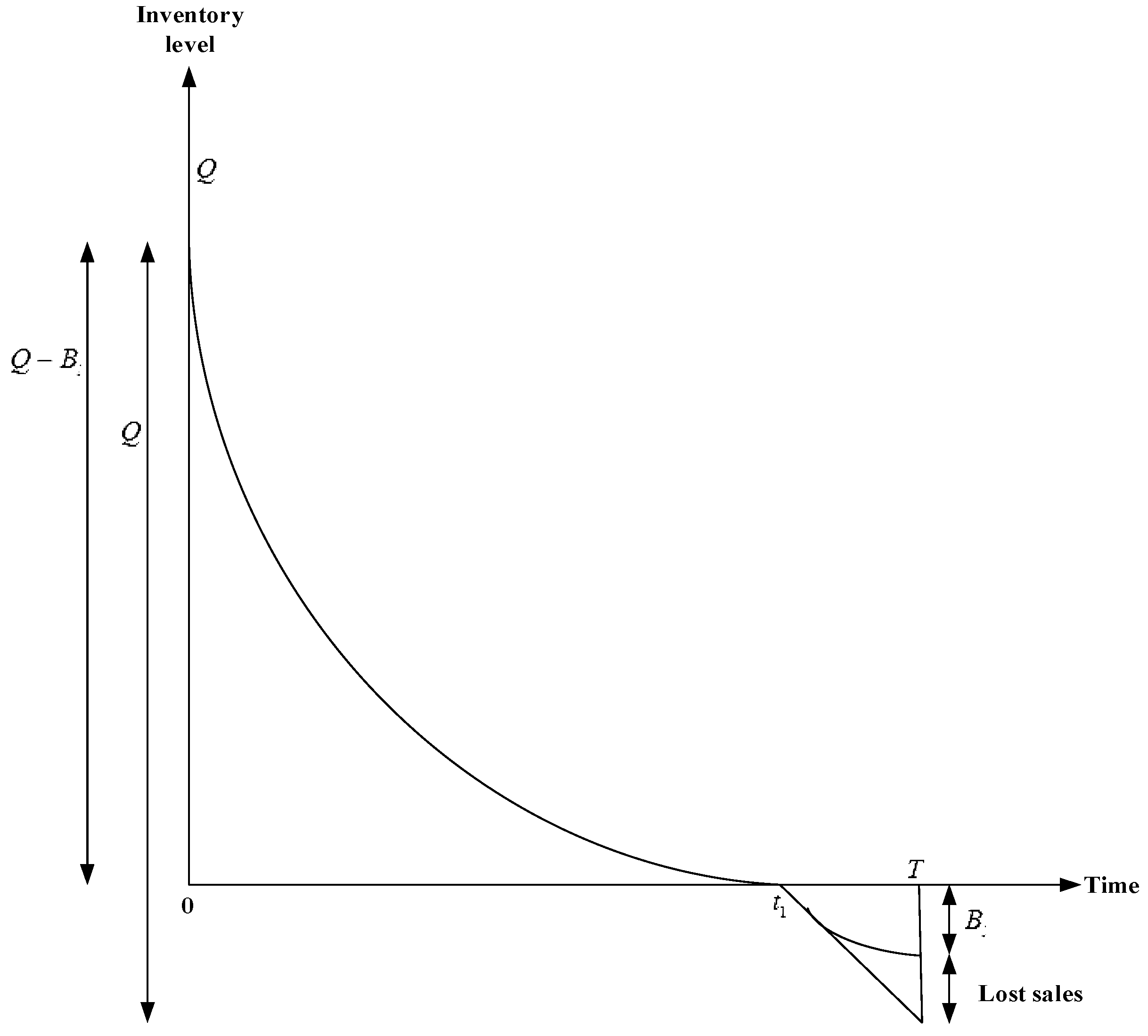
Figure 1. Level of inventory over time T [42].
Mathematics 11 00580 g001
Figure 2. Earned interest and charged interest when ( 0 < M < t 1 ) [42].
Mathematics 11 00580 g002
Figure 3. Interest earned when ( 0 < t 1 < M ) [42].
Mathematics 11 00580 g003
Figure 4. Optimal range of θ when α < 1 for Case (I) and Case (II).
Mathematics 11 00580 g004
Figure 5. Optimal range of θ when α > 1 for Case (I) and Case (II).
Mathematics 11 00580 g005
Figure 6. Decision support system for the retailer.
Mathematics 11 00580 g006
Figure 7. The total cost function’s convexity behavior for α > 0   and   c p > h c .
Mathematics 11 00580 g007
Figure 8. The total cost function’s convexity behavior for α < 0 and cp < hc.
Mathematics 11 00580 g008
Table 1. An overview of similar studies on the EOQ model.
SourceDemandDeteriorationShortages Trade Credit
[12]Ramp typeConstantYesYes
[31]ConstantNoYesYes
[35]ConstantConstantYesYes
[2]Deterioration-dependentControllable deteriorationNoNo
[22]Price- and stock-dependentControllable deteriorationYes No
[24]Constant Weibull deteriorationYesNo
Table 2. Rate of deterioration for different values of α .
α 1 3 1 2 123
θ 0.9630.840.60.3670.263
Table 3. Values of X's, Y's, Z's, and W's.
( a 1 ) = X 1 ( a 2 ) = X 2 ( c p h c ) = X 3 ( h + h c ) = X 4 ( h 2 + h c 2 ) = X 5 ( 2 M 3 S 2 β I e 2 4 M 2 S β c p I e ) = Y 1 ( 4 K M 2 S I e D 0 ) = Y 2 M 2 S 2 β I e 2 = Y 3 ( 2 M S β I e 4 β c p ) = Y 4 M 2 S β I e = Y 5 ( β 2 h c b + β 2 h c c b + β c p D 0 c b β c b D 0 h c ) = Y 6 ( M 3 S 2 β 2 I e 2 + 2 M 2 S c p β 2 I e ) = Y 7 ( β h D 0 + β h c D 0 ) = Y 8 ( β 2 X 5 D 0 2 X 3 2 4 β 2 c b 2 X 1 4 2 β 2 h h c ) = Y 9 ( M 2 S 2 β 2 I e 2 4 M S β 2 c p I e + 4 β 2 c p 2 ) = Y 10 ( β 2 c b h c β c p D 0 c b + β D 0 c b h c + β 2 h c b ) = Z 1 ( 6 M 2 S β I e D 0 + 8 K β ) = Z 2 β D 0 ( c p h h c 2 ) = Z 3 β 2 h h c = Z 4 ( S a 2 β I e + 2 β c b X 1 2 + β X 4 + D 0 X 3 ) = Z 5 ( S a 2 β I e 2 β c b X 1 2 β X 4 D 0 X 3 ) = Z 5 4 β c p X 1 + 2 M S β I e = Z 6 ( 2 S β 2 h I e a 2 4 β 2 c b X 1 2 2 β D 0 X 3 ) = Z 7 ( 2 S β D 0 I e a 2 4 β D 0 c b X 1 2 ) = Z 8 ( D 0 2 X 3 2 β 2 X 4 2 ) = Z 9 16 M S β 2 c p I e X 1 + 4 M 2 S 2 β 2 I e 2 + 16 β 2 c p 2 X 1 2 = Z 10 2 S a 2 β 2 I e D 0 + 4 β D 0 c b X 1 2 2 β D 0 h c + 8 K β = W 1 2 S a 2 β 2 I e + 4 β 2 c b X 1 2 + 4 β 2 = W 2 2 β D 0 ( h c 2 + c p h ) = W 3 ( S 2 a 4 β 2 I e 2 + 4 S β 2 I e c b ( a X 1 ) 2 + 4 β 2 c b 2 X 1 4 ) = W 4
Table 4. Sensitivity analysis.
ParametersValues                   T   ( in   Years )           θ ( in   % )                 Q   ( in   Units )                 t 1   ( in   Years )       T C ( in   USD )             γ ( in   % )
α 3.20.2200.7025.160.176667.840.021
3.60.2220.6425.570.178667.050.026
4.40.2260.5526.230.181665.450.031
4.80.2280.5126.490.182664.680.033
D 0 800.2360.6623.940.189606.970.011
900.2360.6624.140.189611.950.014
1100.2140.5527.450.171719.160.041
1200.2050.5228.840.164771.010.051
K 320.1660.6522.730.159628.490.015
360.2120.6124.390.170647.940.023
440.2360.5727.360.189683.610.034
480.2470.5628.730.198700.170.039
β 120.2250.4926.610.180674.780.066
13.50.2250.5326.330.180670.710.048
16.50.2220.6925.150.178661.140.009
184.8474.429.243.87741019.31136.543
c p 80.2161.2123.640.172584.010.002
90.2101.2422.890.162618.440.003
110.1961.3421.000.157712.130.013
120.1901.3820.220.152754.200.020
h 80.2400.5527.850.192645.880.043
90.2320.5726.850.185656.240.036
110.2220.6025.660.178669.170.026
120.2120.6524.240.169685.230.016
h c 6.40.2260.5526.210.181665.690.043
7.20.2260.5726.010.180666.060.033
8.80.2061.1422.610.164669.830.0005
9.60.2061.1522.590.164669.830.0005
M 0.160.2240.6025.840.179677.140.025
0.180.2240.6025.880.179671.700.027
0.220.2250.5825.960.180660.790.031
0.240.2250.5726.000.180655.330.033
I e 0.080.2270.5926.210.182673.200.028
0.090.2260.5926.060.181669.730.028
0.110.2230.5925.790.179662.750.030
0.120.2220.5925.690.178660.300.030
S 240.2270.5926.210.182673.200.028
270.2260.5926.060.181669.730.028
330.2230.5925.790.179662.750.030
360.2220.5925.690.178660.300.030
Disclaimer/Publisher’s Note: The statements, opinions and data contained in all publications are solely those of the individual author(s) and contributor(s) and not of MDPI and/or the editor(s). MDPI and/or the editor(s) disclaim responsibility for any injury to people or property resulting from any ideas, methods, instructions or products referred to in the content.