Existence of Self-Excited and Hidden Attractors in the Modified Autonomous Van Der Pol-Duffing Systems

Abstract

This study investigates the multistability phenomenon and coexisting attractors in the modified Autonomous Van der Pol-Duffing (MAVPD) system and its fractional-order form. The analytical conditions for existence of periodic solutions in the integer-order system via Hopf bifurcation are discussed. In addition, conditions for approximating the solutions of the fractional version to periodic solutions are obtained via the Hopf bifurcation theory in fractional-order systems. Moreover, the technique for hidden attractors localization in the integer-order MAVPD is provided. Therefore, motivated by the previous discussion, the appearances of self-excited and hidden attractors are explained in the integer- and fractional-order MAVPD systems. Phase transition of quasi-periodic hidden attractors between the integer- and fractional-order MAVPD systems is observed. Throughout this study, the existence of complex dynamics is also justified using some effective numerical measures such as Lyapunov exponents, bifurcation diagrams and basin sets of attraction.

1. Introduction

Recently, fractional analysis (FA) has received increasing interest owing to its usefulness in various fields of science and technology [1]. For example, FA has potential applications in image processing [2], heat transfer [3], food web models [4], thermoelectricity models [5,6], biological models [7,8], physical models [9,10], image encryption algorithm [11] and some models of the financial market [12].

In 2008, Matouk and Agiza introduced a new system that describes the dynamics of the modified autonomous Van der Pol-Duffing oscillator [13], or simply the MAVPD system. The proposed MAVPD equations are described by a system of three coupled ordinary differential equations (ODEs) with a single cubic nonlinearity. In [13], conditions of Hopf bifurcations and chaos synchronization were studied via the backstepping design approach. Afterward, the MAVPD system received increasing attention from scientists owing to its simple form, variety of rich, complex dynamics and ease of implementation in engineering applications. For example, in [14], Fan presented a computer-assisted proof for the existence of chaos in the MAVPD system based on the topological horseshoe theorem. In [15], Braga et al. studied the local codimension 1, 2 and 3 bifurcations in the MAVPD system. In [16], Wang and Li used an adaptive pulse perturbation scheme to control chaos in the MAVPD system; they also presented a scheme of measuring the frequency of weak sinusoidal signal based on this system [17]. In [18], Zhao et al. studied hidden attractors in a generalized version of the MAVPD system. In [19], El-Sayed et al. investigated the conditions of pitchfork bifurcation in the MAVPD system based on the center manifold theory. In [20], Cai et al. investigated the conditions of Hopf bifurcation control in the MAVPD system. In [21], Zhou et al. investigated the conditions of Hopf bifurcation in the MAVPD system based on calculations of the first Lyapunov coefficients. In [22], Han et al. studied two novel delay-induced bursting patterns in the MAVPD system. In [23], Zhang et al. investigated bursting oscillations in a modified three-dimensional version of the van der Pol-Duffing circuit.

On the other hand, the FA of the MAVPD system has received increasing attention. In [24], Matouk investigated the local stability conditions and chaotic dynamics in a fractional-order version of the MAVPD system. Chaos synchronization was also studied in the fractional MAVPD system via Takagi-Sugeno fuzzy approaches and backstepping control [25].

The problems of investigating self-excited and hidden attractors in integer and fractional-order systems have received growing interest from authors [26,27,28]. This line of research has potential applications in industry, secure communications, and chaos-based applications. In [28], Almatroud et al. investigated the multistability and coexisting hidden chaotic attractors in the fractional-order Matouk’s system. In fact, the problem of the phase transition of complex dynamics between the integer-order system and its fractional counterpart is still under development. Most of the literature on the topic asserts that integer-order chaotic systems have fractional-order chaotic counterparts. In [29], Matouk provided an example of hidden chaotic attractors that exist only in the fractional-order Matouk’s system when using a specific choice of parameter values and initial conditions.

Here, we discuss the multistability and coexisting attractors in the integer- and fractional-order MAVPD systems due to the appearances of hidden and self-excited attractors. Our novel foundations can be outlined as follows: (i) coexistence of self-excited chaotic (or non-chaotic) attractors and periodic orbits are found in the integer-order MAVPD system; (ii) coexistence of hidden periodic (or quasi-periodic) attractors and periodic orbits are found in the integer-order MAVPD system; (iii) coexistence of hidden quasi-periodic attractors and chaotic attractors are found in the integer-order MAVPD system and (iv) coexistence of hidden quasi-periodic attractors and chaotic attractors are found in the fractional-order MAVPD system. Moreover, the existence of self-excited attractors in the fractional-order MAVPD is observed. For these reasons, the conditions for Hopf bifurcation in the MAVPD systems are studied in the integer- and fractional-order cases. Furthermore, the technique for hidden attractors localization in the integer-order MAVPD is provided to enhance the theoretical framework in this study.

The study is divided into eight sections as follows. The introductory part is provided in Section 1. The preliminary part is provided in Section 2. The system’s description is explained in Section 3. Hopf bifurcation’s discussion for the integer-order MAVPD system and its fractional counterpart is provided in Section 4. The theoretical framework for localizing the hidden oscillation in the integer-order MAVPD system is explained in Section 5. Numerical examples for the existence of self-excited and hidden attractors in the integer-order MAVPD system and its fractional version are, respectively, provided in Section 6 and Section 7. The Section 8 is devoted to drawing the conclusions for this work.

2. Preliminaries

A formal definition of fractional derivative, which is widely applied in several fields of science, was introduced by Caputo [30] as follows

$${}_{\tau }{}^{C}D_{t_0}^q\beta (\tau )=\left({\displaystyle \underset{t_0}{\overset{\tau }{\int }}{(\tau -\mu )}^{m-q-1}{\beta }^{(m)}(\mu )d\mu }\right)/\Gamma (m-q), \tau >0,$$

(1)

where $m-1<q<m, m\in N,$$\Gamma (.)$ is the classic Gamma function and ${\beta }^{(m)}(\mu )=\frac{d^m\beta (\mu )}{d{\mu }^m}$.

The stability problem of a linearized fractional-order n-dimensional system was introduced by Matignon [31] as follows

$$q<\frac{2}{\pi }\left|\arg ({\lambda }_j)\right|, j=1,\dots ,n,$$

(2)

where ${\lambda }_j$ is an eigenvalue of the linearized system’s Jacobin matrix. In other words, an equilibrium point of the fractional-order dynamical system is locally asymptotically stable (LAS) if the Conditions (2) hold. Afterwards, further investigations of such a stability problem were studied in [32,33].

The hidden attractors’ problem is an old topic of dynamical systems, since it arose in the early 20th century by David Hilbert, in association with the second part of Hilbert’s sixteenth problem for investigating hidden periodic oscillations [34]. Additionally, this kind of study deals with the investigation of mutual disposition and the number of limit cycles in two-dimensional polynomial systems that are modeled by ODEs [35]. A formal definition of hidden and self-excited attractors is described as follows:

Definition 1

([26]). A self-excited attractor is an attractor whose basin of attraction intersects with any open neighborhood of an equilibrium point ($\overline{P}$); however, the basin set of attraction of a hidden attractor is not connected with any small neighborhood of $\overline{P}$.

Thus, attractors are divided into hidden and self-excited types in dynamical systems, especially those with no equilibria and those with unique stable $\overline{P}$.

3. The MAVPD Systems

The integer-order MAVPD equations [13] are modeled by:

$$\begin{array}{l}{\dot{y}}_1=-\delta (-\gamma y_1-y_2+y_1^3),\\ {\dot{y}}_2=y_1-\xi y_2-y_3, \\ {\dot{y}}_3=\rho y_2,\end{array}$$

(3)

where $y_i, i=1,2,3$ represents a system’s state variable and the system’s parameters are $\delta , \rho , \xi \in R^{+}$ and $\gamma \in R.$ The MAVPD system has the equilibria ${\overline{P}}_1=(0,0,0)$ and ${\overline{P}}_{2,3}=(\pm \sqrt{\gamma },0,\pm \sqrt{\gamma }).$ Furthermore, the system (3) exhibits a variety of rich complex dynamics including periodic, quasi-periodic, and chaotic behaviors. Figure 1 shows the evidence for the existence of such rich dynamics via calculations of the model’s Lyapunov spectrum (See Ref. [36]), fixing the parameter values at $\gamma =0.1, \delta =100, \rho =200$ and varying $\xi$. Moreover, the related calculation of the model’s bifurcation diagram is depicted in Figure 2.

Finally, a fractional-order version of the system (3), in the Caputo sense, is also described by

$$\begin{array}{l}{}_t{}^{C}D_0^q{y}_1=-\delta (-\gamma y_1-y_2+y_1^3),\\ {}_t{}^{C}D_0^q{y}_2=y_1-\xi y_2-y_3, \\ {}_t{}^{C}D_0^q{y}_3=\rho y_2.\end{array}$$

(4)

4. Discussion on Hopf Bifurcation in the MAVPD Systems

Firstly, the classic Routh–Hurwitz conditions can be utilized to show that the origin equilibrium point of system (3) with $\gamma <0$ is LAS iff

$${\xi }_0=\frac{-(\rho -\delta +{\gamma }^2{\delta }^2)+\sqrt{{(\rho -\delta +{\gamma }^2{\delta }^2)}^2+4{\gamma }^2{\delta }^3}}{-2\gamma \delta }>0.$$

(5)

However, when $\gamma >0$, the other non-origin equilibrium points ${\overline{P}}_{2,3}=(\pm \sqrt{\gamma },0,\pm \sqrt{\gamma })$ appear and become LAS iff

$${\xi }_1=\frac{-(\rho -\delta +4{\gamma }^2{\delta }^2)+\sqrt{{(\rho -\delta +4{\gamma }^2{\delta }^2)}^2+16{\gamma }^2{\delta }^3}}{4\gamma \delta }>0.$$

(6)

To discuss the existence of Hopf bifurcation in system (3), we recall the following theorems [13,19]:

Theorem 1.

The MAVPD system (3) exhibits a Hopf bifurcation at${\overline{P}}_1=(0,0,0)$for$\rho >0, \delta >0$and$\gamma <0$in the neighborhood of ($\xi ={\xi }_0$). Furthermore, by setting$\psi ={\xi }_0^2-\delta -2\gamma \delta {\xi }_0$, the bifurcation type can be classified as follows; (i) if$\psi >0$, the bifurcation is supercritical. (ii) if$\psi <0$, the bifurcation is subcritical.

Theorem 2.

The MAVPD system (3) exhibits a Hopf bifurcation at${\overline{P}}_{2,3}=(\pm \sqrt{\gamma },0,\pm \sqrt{\gamma })$for$\rho >0, \delta >0$and$\gamma >0$in the neighborhood of ($\xi ={\xi }_1$). Furthermore, (i) if$\eta >0$, the bifurcation is supercritical. (ii) if$\eta <0$, the bifurcation is subcritical, where$\eta$is the left-hand side of Equation (13) in Ref. [19].

For $q\in (0,1)$, the fractional-order system cannot exhibit periodic solutions according to the proof given in [37]. Hence, the theory of Hopf bifurcation in fractional-order systems is only used to obtain an approximation to the periodic solutions. In the following, we first consider the case of ${\overline{P}}_1$ whose eigenvalue equation is described as

$$\varphi (\lambda )={\lambda }^3+(\xi -\gamma \delta ){\lambda }^2+(\rho -\delta -\xi \gamma \delta )\lambda -\gamma \delta \rho =0.$$

(7)

Obviously, ${\overline{P}}_1$ has a pair of complex conjugate eigenvalues ${\lambda }_{1,2}=\sigma \pm i\theta$ and one real eigenvalue ${\lambda }_0$ when the discriminant of $\varphi (\lambda )$ is a negative real value. Then, we define the function $\Lambda (q)=\frac{q\pi }{2}-{\tan }^{-1}(\frac{\theta }{\sigma }),$ where ${\sigma }^2+{\theta }^2=\chi , {\chi }^3+(\delta -\rho +\xi \gamma \delta ){\chi }^2+\delta \gamma \rho (\delta \gamma -\xi )\chi -{\rho }^2{\gamma }^2{\delta }^2=0$. Therefore, the origin point ${\overline{P}}_1=(0,0,0)$ changes its stability near the critical value of the fractional parameter $q_c^{(1)}=\frac{2}{\pi }{\sec }^{-1}(\frac{\sqrt{\chi }}{\sigma }).$ It is also evident that ${\frac{d\Lambda (q)}{dq}|}_{q=q_c^{(1)}}=\frac{\pi }{2}\ne 0$.

Finally, we consider the case of the non-origin points ${\overline{P}}_{2,3}=(\pm \sqrt{\gamma },0,\pm \sqrt{\gamma })$ whose critical value of the fractional parameter is calculated as follows

$$q_c^{(2)}=\frac{2}{\pi }{\sec }^{-1}(\frac{\sqrt{{\chi }^{\prime }}}{{\sigma }^{\prime }}),{{\sigma }^{\prime }}^2+{{\theta }^{\prime }}^2={\chi }^{\prime }, {{\chi }^{\prime }}^3-(\rho -\delta +2\xi \gamma \delta ){{\chi }^{\prime }}^2+2\delta \gamma \rho (2\delta \gamma +\xi ){\chi }^{\prime }-4{\rho }^2{\gamma }^2{\delta }^2=0,$$

(8)

where ${\sigma }^{\prime }, {\theta }^{\prime }$ are, respectively, the real and imaginary parts of the two pairs of the eigenvalues corresponding to the non-origin points ${\overline{P}}_{2,3}=(\pm \sqrt{\gamma },0,\pm \sqrt{\gamma }).$

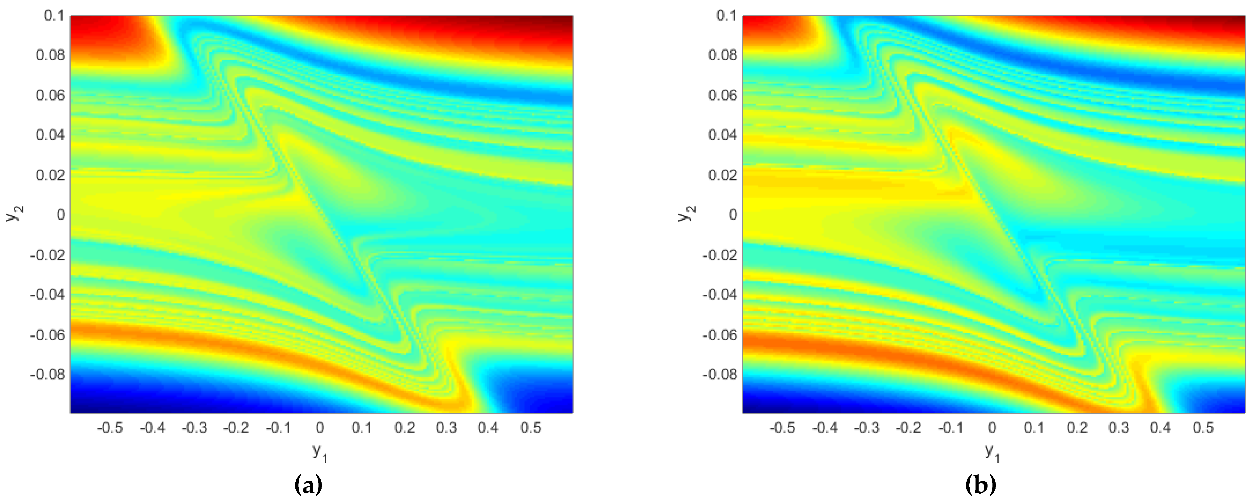
5. Hidden Oscillation Localization

Here, we will employ the algorithm presented in [38] that can be used to localize hidden oscillations. Firstly, we consider that the MAVPD system is written on the Lur’e form

$$\frac{d\mathrm{Y}}{dt}=\mathrm{M}\mathrm{Y}+\Theta \zeta (s^{*}\mathrm{Y}),$$

(9)

where $\mathrm{Y}\in R^3, \mathrm{M}=\left(\begin{array}{ccc}\delta \gamma & \delta & 0\\ 1& -\xi & -1\\ 0& \rho & 0\end{array}\right), \zeta (\sigma )={\sigma }^3, \Theta =-\delta \left(\begin{array}{c}1\\ 0\\ 0\end{array}\right), s=-\left(\begin{array}{c}1\\ 0\\ 0\end{array}\right).$

Now, let $\alpha$ denote the coefficient of harmonic linearization, ${\omega }_0>0$ denote the starting frequency and the parameter $\epsilon$ denote a small enough positive value, then system (9) can be written as

$$\frac{d\mathrm{Y}}{dt}={\mathrm{M}}_0\mathrm{Y}+\Theta \epsilon \phi (s^{*}\mathrm{Y}),$$

(10)

where ${\mathrm{M}}_0=\left(\begin{array}{ccc}\delta (\gamma +\alpha )& \delta & 0\\ 1& -\xi & -1\\ 0& \rho & 0\end{array}\right), {\lambda }_{1,2}^{{\mathrm{M}}_0}=\pm i{\omega }_0, {\lambda }_3^{{\mathrm{M}}_0}=-d<0, \phi (\sigma )=\zeta (\sigma )-\alpha \sigma .$

Then, we consider the non-singular linear transformation $\mathrm{Y}=S\mathrm{Z}$ that transforms the system (10) into

$$\frac{d\mathrm{Z}}{dt}=\mathrm{T}\mathrm{Z}+\mathrm{B}\epsilon \phi (U^{*}\mathrm{Z}),$$

(11)

where $\mathrm{T}=\left(\begin{array}{ccc}0& -{\omega }_0& 0\\ {\omega }_0& 0& 0\\ 0& 0& -d\end{array}\right), \mathrm{B}=\left(\begin{array}{c}{b}_1\\ b_2\\ 1\end{array}\right), U=\left(\begin{array}{c}1\\ 0\\ -h\end{array}\right).$

According to [38], the transfer function $W_{{\rm T}}(p)$ of system (11) is described as

$$W_{\mathrm{T}}(p)=\frac{h}{d+p}+\frac{{\omega }_0{b}_2-p{b}_1}{{\omega }_0^2+p^2},$$

(12)

where $p$ is a complex variable. Moreover, according to [38], the equality of transfer functions of Equations (10) and (11)

$$W_{\mathrm{T}}(p)=s^{*}({{\mathrm{M}}_0-p\mathrm{I})}^{-1}\Theta$$

(13)

leads to the following calculations

$$\begin{array}{l}\alpha =\frac{\rho -\delta -\delta \gamma \xi -{\omega }_0^2}{\xi \delta }, d=\frac{\delta -\rho +{\xi }^2+{\omega }_0^2}{\xi }, h=\frac{\delta (\rho +d^2-\xi d)}{d^2+{\omega }_0^2},\\ b_1=\frac{\delta (\rho -{\omega }_0^2-\xi d)}{d^2+{\omega }_0^2}, b_2=\frac{\delta d(\rho -{\omega }_0^2)}{(d^2+{\omega }_0^2){\omega }_0}.\end{array}$$

(14)

As we know, the above-mentioned non-singular transformation $\mathrm{Y}=S\mathrm{Z}$ can reduce system (10) to the form (11) given that

$$\mathrm{T}=S^{-1}{\mathrm{M}}_{0}S, \mathrm{B}=S^{-1}\Theta , U^{*}=s^{*}S,$$

(15)

where the non-singular matrix $S$ has the following form

$$S=\left(\begin{array}{ccc}1& 0& -h\\ -(\gamma +\alpha )& -\frac{{\omega }_0}{\delta }& \frac{h(d+\delta (\gamma +\alpha ))}{\delta }\\ \frac{\rho }{\delta }& -\frac{\rho (\gamma +\alpha )}{{\omega }_0}& -\frac{\rho h(d+\delta (\gamma +\alpha ))}{\delta d}\end{array}\right).$$

Then, for the sake of localization of the hidden oscillation, the following set of initial conditions can be chosen (when $\epsilon$ is small enough)

$$\mathrm{Z}(0)=\left(\begin{array}{c}{z}_1(0)\\ z_2(0)\\ z_3(0)\end{array}\right)=\left(\begin{array}{c}{a}_0\\ 0\\ 0\end{array}\right)$$

(16)

for the first step of the multistep procedure. So, the relations between the initial conditions of systems (10) and (11) can be expressed with the aid of (16) as follows

$$\mathrm{Y}(0)=S\mathrm{Z}(0)=S\left(\begin{array}{c}{a}_0\\ 0\\ 0\end{array}\right)=\left(\begin{array}{c}{a}_0\\ -\left(\gamma +\alpha \right)a_0\\ \frac{\rho a_0}{\delta }\end{array}\right)$$

(17)

where $a_0$ is obtained from the describing function [38]

$$\Phi (a)={\displaystyle \underset{0}{\overset{2\pi /{\omega }_0}{\int }}\left[{\phi }_1((\cos {\omega }_{0}t)a,(\sin {\omega }_{0}t)a,0)\cos {\omega }_{0}t+{\phi }_2((\cos {\omega }_{0}t)a,(\sin {\omega }_{0}t)a,0)\sin {\omega }_{0}t\right]dt},$$

(18)

given that $\Phi (a_0)=0$ and the quantity $({\Phi }^{\prime }(a_0))b_1$ is not vanished, where the dash refers to the first integer-order derivative.

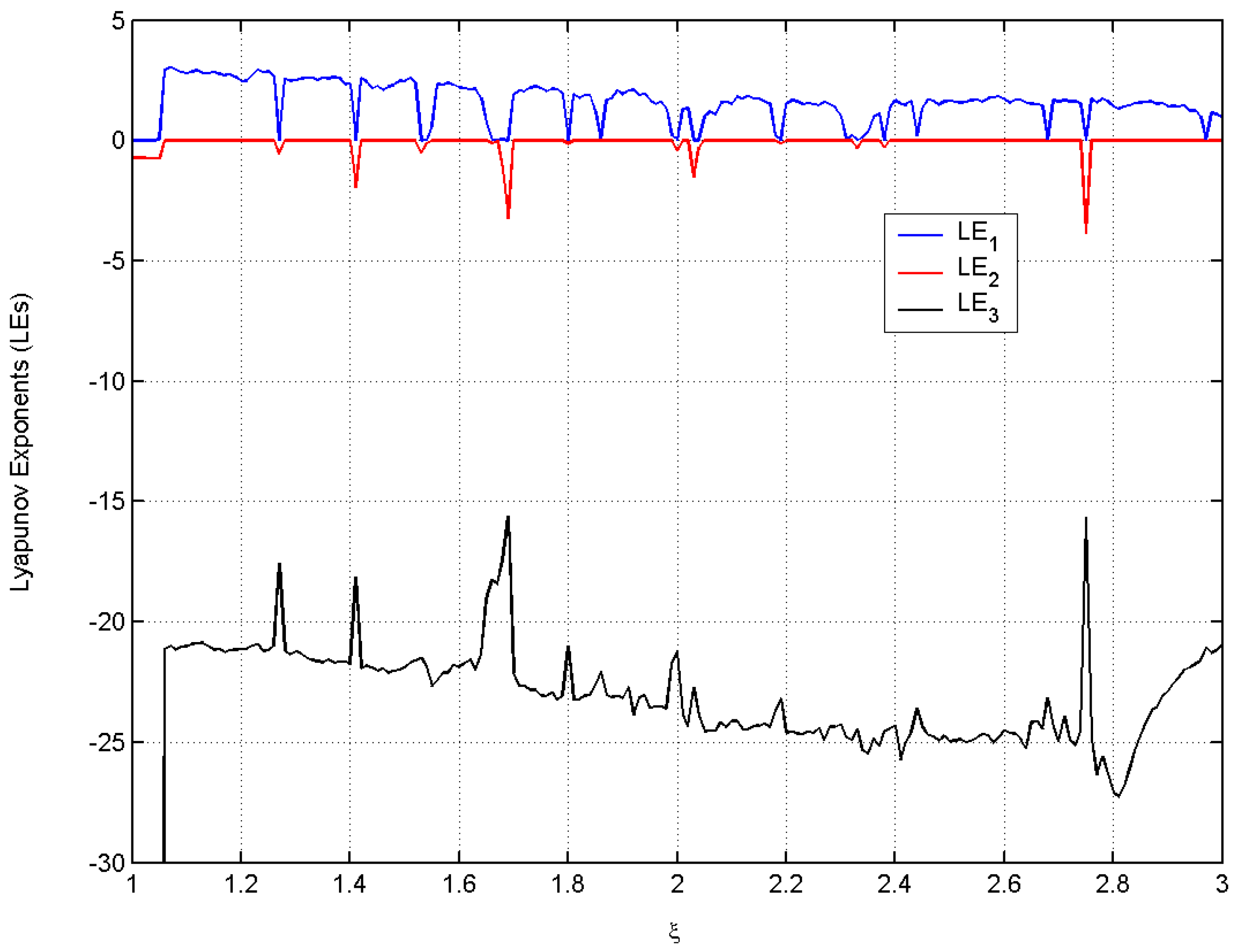
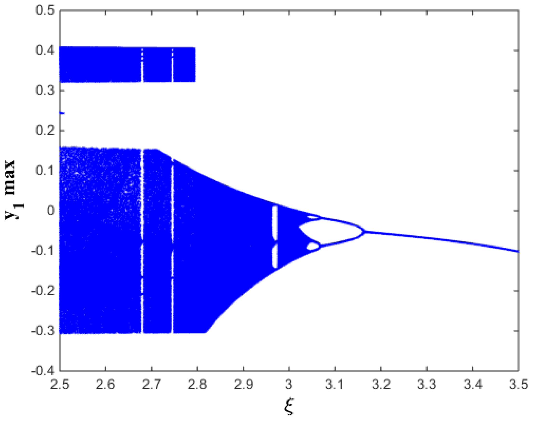
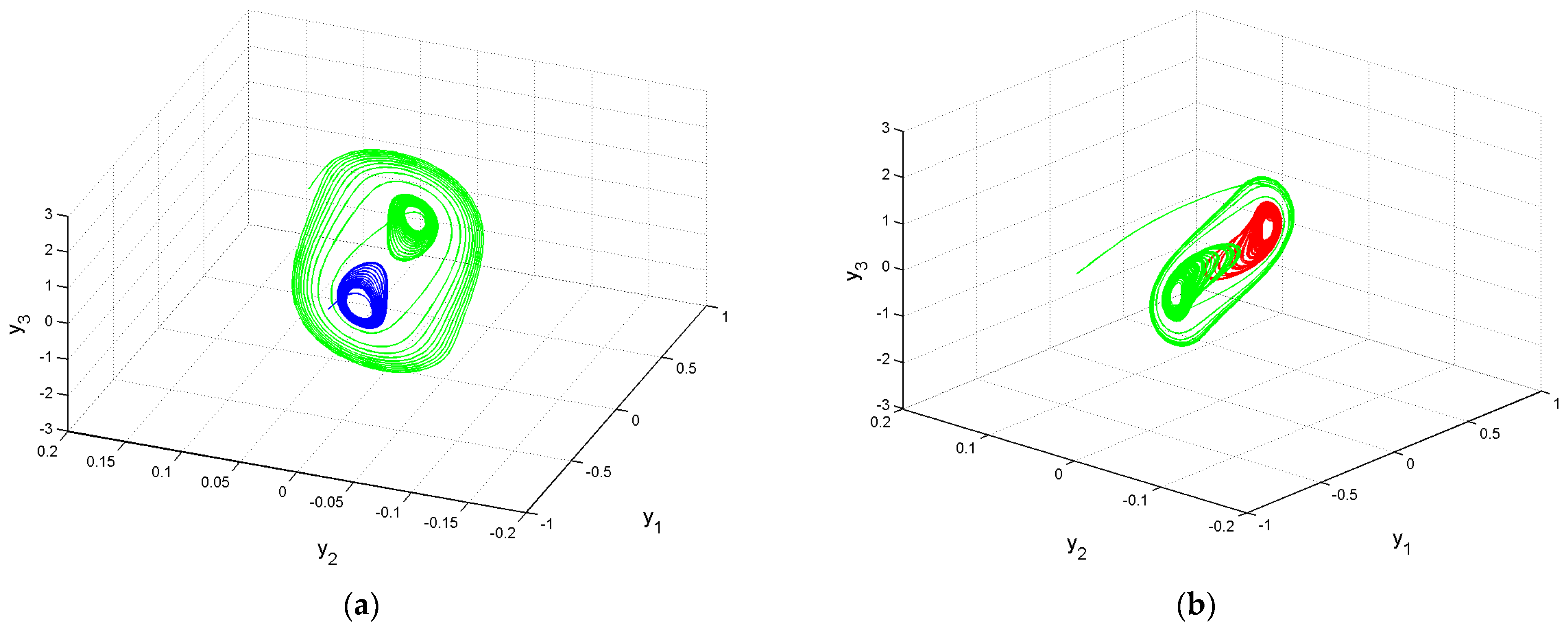
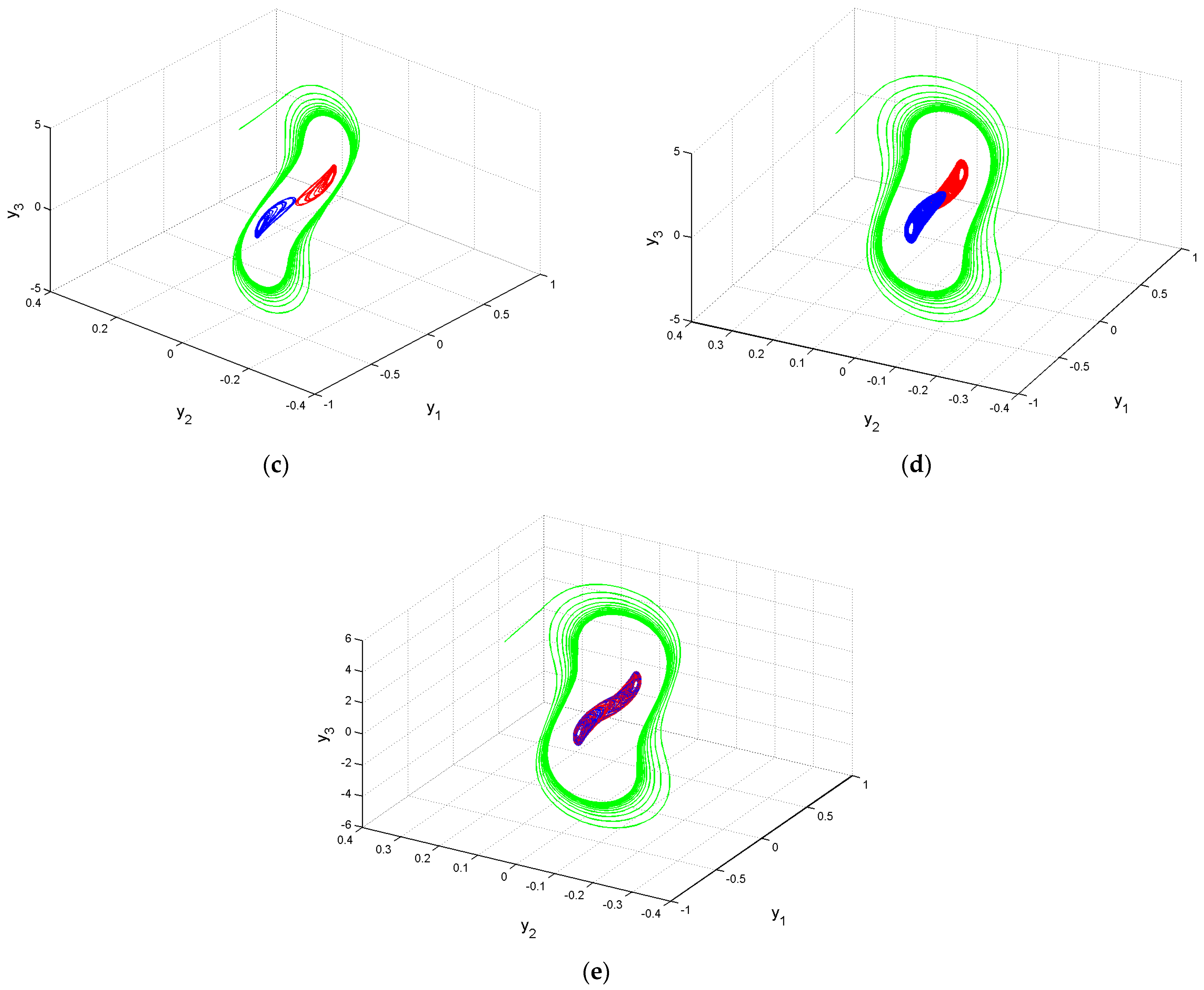
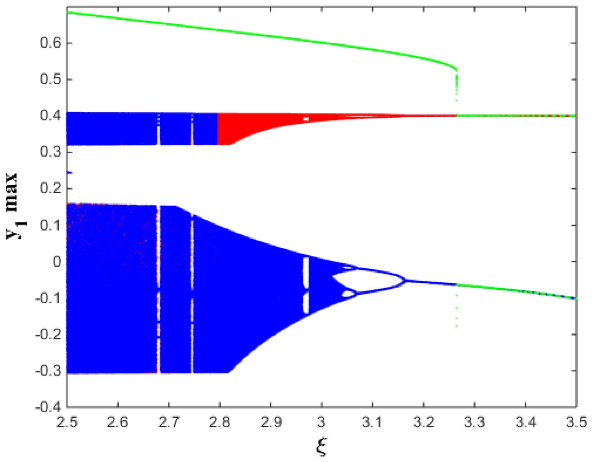
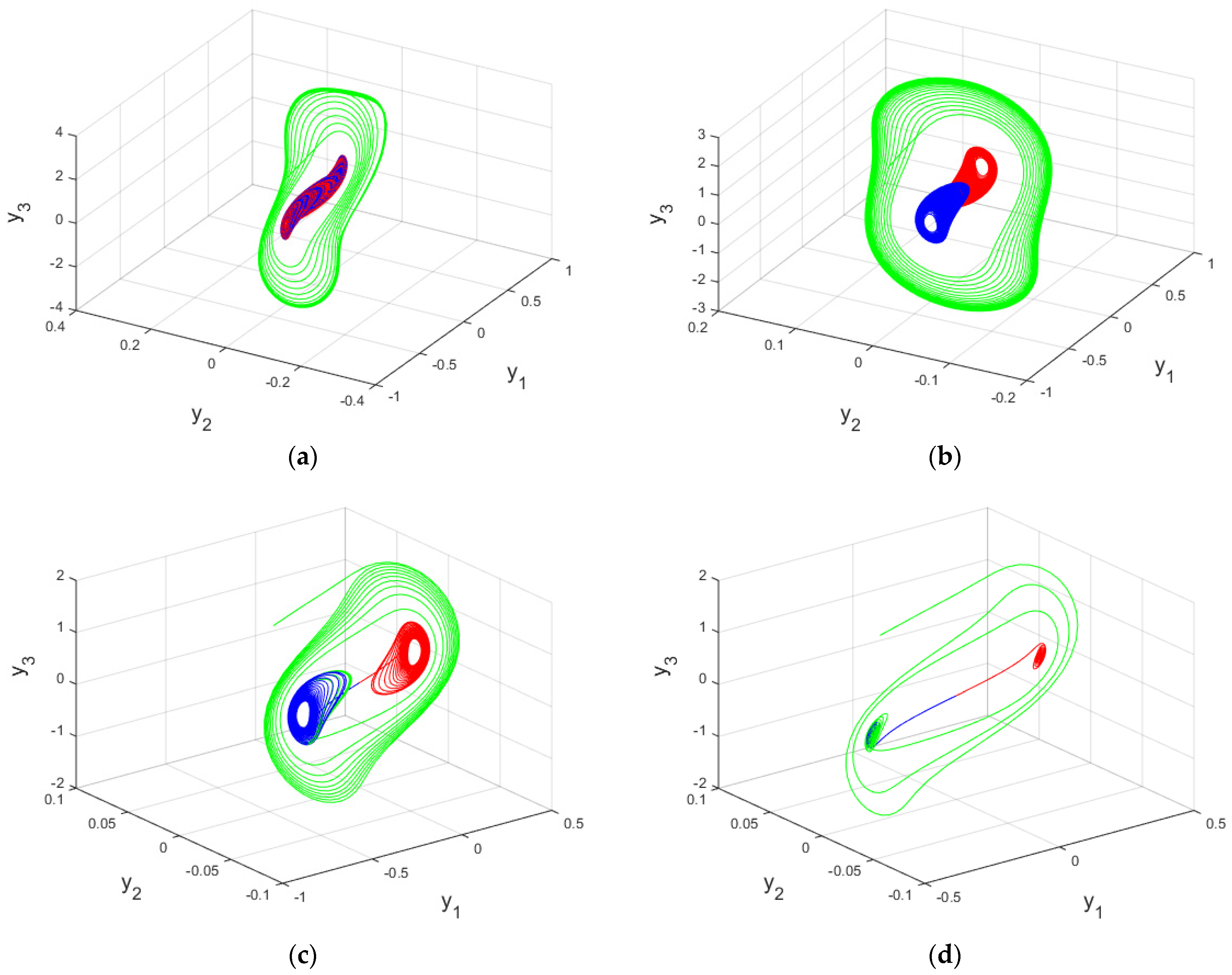
6. Existence of Self-Excited and Hidden Attractors in the Integer-Order MAVPD System

In the following, we will discuss some complex dynamics in the integer-order MAVPD system. The simulation results are performed based on the MATLAB command ODE45 with a relative error tolerance of 1e-4. We will also consider the parameter $\xi$ as the dynamical parameter and use the above-mentioned values of the other parameters. So, the critical Hopf bifurcation value is ${\xi }_1=3.5078$ and ${\overline{P}}_{2,3}$ are LAS if and only if $\xi >{\xi }_1$. For $\xi =3.4,$ coexistence of self-excited attractor and a limit cycle is found. For $\xi =2.85,$ coexistence of self-excited chaotic attractor and one-scroll chaotic attractor around ${\overline{P}}_2$ is found. The results are illustrated in Figure 3 in which the self-excited attractors have the green domain.

On the other hand, hidden attractors exist in this system where their initial conditions are selected based on the above-mentioned analysis. For example, when $\xi =3.5,$ the coexistence of a hidden periodic attractor surrounds the limit cycle that bifurcates from ${\overline{P}}_2$ and a limit cycle around ${\overline{P}}_3$ is observed. When $\xi =3.1,$ the existence of a hidden quasi-periodic attractor surrounds the coexisting two period-2 limit cycles that bifurcate from ${\overline{P}}_2$ and ${\overline{P}}_3$, is observed. When $\xi =3.05,$ the existence of a hidden quasi-periodic attractor surrounds the coexisting two period-4 limit cycles that bifurcate from ${\overline{P}}_2$ and ${\overline{P}}_3$, is observed. When $\xi =2.85,$ the existence of a hidden quasi-periodic attractor that surrounds the coexisting two one-band chaotic attractors, is found. Finally, when $\xi =2.6,$ the existence of a hidden quasi-periodic attractor that surrounds the double-band chaotic attractors is found. The explanation is given as follows; when the dynamical parameter lies below its critical value ${\xi }_1=3.5078$, the two non-origin points ${\overline{P}}_2$ and ${\overline{P}}_3$ change their stability to the saddle type of index 2. In this case, the origin point is also the saddle point of index 2. Hence, any trajectory originating from the initial states given in

Table 1. Calculations of the initial conditions for locating hidden oscillations in the MAVPD system (3).

Bifurcation Parameter $\mathit{\xi }$	${\mathit{\omega }}_0$	$\mathit{\alpha }$	Initial Conditions
$\xi =3.5$	10.2344	0.1136	${[0.3651, 0.005, 0.7303]}^T$
$\xi =3.1$	18.6143	0.8951	${[0.3651, 0.2903, 0.7303]}^T$
$\xi =3.05$	18.6261	0.9096	${[0.3651, 0.2956, 0.7303]}^T$
$\xi =2.85$	18.6711	0.9723	${[0.3651, 0.3185, 0.7303]}^T$
$\xi =2.6$	18.7228	1.0636	${[0.3651, 0.3519, 0.7303]}^T$

will not converge to any of these equilibria or the unstable periodic orbits bifurcating from ${\overline{P}}_1$ and ${\overline{P}}_2$ and ${\overline{P}}_3$ due to the existence of subcritical Hopf bifurcation around all these points. Thus, the hidden attractors occur because the trajectories originate from the above-mentioned initial states cannot be initiated from the point of an unstable manifold in the neighborhoods of ${\overline{P}}_1$, ${\overline{P}}_2$ and ${\overline{P}}_3$. Figure 4 summarizes all these results in which the hidden attractors are shown (green domain) and the initial conditions ${[1\times {10}^{-5}, 0, 1\times {10}^{-5}]}^T$, ${[-1\times {10}^{-5}, 0, -1\times {10}^{-5}]}^T$ are associated with the red and blue attractors, respectively. Moreover, based on the above-mentioned analysis in Section 5, the selection of the initial conditions corresponding to hidden attractors are specified in the following table.

The corresponding bifurcation diagrams are depicted in Figure 5, in which a route to chaos via period-doubling bifurcation is shown. The last figure shows that all the points ${\overline{P}}_1$, ${\overline{P}}_2$ and ${\overline{P}}_3$ lose their stability below the value ${\xi }_1\approx 3.51$ where subcritical Hopf bifurcation around the non-origin points takes place. It is also shown that the coexistence of a quasi-periodic hidden attractor (green plot) and periodic orbits (blue and red plots) is found when $\xi \in (3.04,3.51)$ and the coexistence of a quasi-periodic hidden attractor (green plot) and chaotic attractors (blue and red plots) is found when $\xi \in (2.5,3.04)$.

We also carried out computations for the system’s basin sets of attraction (BSA) that are useful to illustrate the existence of the hidden attractors and coexistence of multi-attractors. In Figure 6, we use the parameters $\gamma =0.1, \delta =100, \rho =200$ and vary $\xi$. The BSA in part a of Figure 6 depicts the regions of hidden quasi-periodic attractors (red and blued domains) and the coexisting two one-band chaotic attractors around ${\overline{P}}_2$ (turquoise domain) and ${\overline{P}}_3$ (yellow domain). The BSA in part b of Figure 6 depicts the regions of hidden quasi-periodic attractors (red and blued domains) and the coexisting two periodic orbits around ${\overline{P}}_2$ (turquoise domain) and ${\overline{P}}_3$ (yellow domain).

7. Existence of Self-Excited and Hidden Attractors in the Fractional-Order MAVPD System

For $\gamma =0.1, \delta =100, \rho =200$ and $\xi =1.6$, system (4) is numerically integrated using the PECE method [1] with a step size of 0.01 and with different values of the fractional orders. In this case, based on condition (2), all the equilibrium points are not LAS when q is greater than 0.9586. In addition, the critical value for the approximating periodic solution around the non-origin points ${\overline{P}}_2$ and ${\overline{P}}_3$ is $q_c^{(2)}\approx 0.96$. On the other hand, motivated by the above-mentioned discussion, double-band chaos around all the equilibria and/or one-band chaos around each of the non-origin equilibria is expected when 1 < q < 0.96. Therefore, hidden attractors may appear for 1 < q < 0.96 as the trajectories originate near the approximating periodic (or quasi-periodic) trajectories cannot be initiated from the point of an unstable manifold in the neighborhoods of ${\overline{P}}_1$, ${\overline{P}}_2$ and ${\overline{P}}_3$. The results are outlined in Figure 7 where the initial conditions are selected as ${[1\times {10}^{-1}, 1\times {10}^{-1},1\times {10}^{-1}]}^T$ for the green domain, ${[1\times {10}^{-5}, 0, 1\times {10}^{-5}]}^T$ for the red domain and ${[-1\times {10}^{-5}, 0, -1\times {10}^{-5}]}^T$ for the blue domain. This figure shows that a hidden quasi-periodic attractor surrounding a double-band chaotic attractor exists when $q=0.98;$ A hidden quasi-periodic attractor surrounding the coexisting two one-band chaotic attractors exists when $q=0.97;$ A self-excited quasi-periodic attractor surrounding the coexisting two periodic attractors near ${\overline{P}}_2$ and ${\overline{P}}_3$ exists when $q=0.96$ and a self-excited attractor surrounding the coexisting two asymptotic attractors near ${\overline{P}}_2$ and ${\overline{P}}_3$ exists when $q=0.94$.

The corresponding bifurcation diagrams are depicted in Figure 8 in which a route to chaos is observed. This bifurcation diagram shows that all the equilibria lose their stability when $q$ passes forward $0.9586$. Then, approximating periodic trajectories are shown when $q$ becomes near the critical value $q_c^{(2)}\approx 0.96$. Moreover, it is also shown that a self-excited attractor (green plot) and approximating periodic trajectories (blue and red plots) are found when $q\in (0.9,0.965]$ and the coexistence of a quasi-periodic hidden attractor (green plot) and chaotic attractors (blue and red plots) is found for $q\in (0.967,0.99).$ Furthermore, the figure shows that the indicated hidden attractor disappears for $q\in [0.99,1].$

8. Conclusions

In this study, the multistability and coexisting attractors in the MAVPD systems due to the appearances of hidden and self-excited attractors have been studied in the integer- and fractional-order cases. The analytical conditions for the existence of periodic solutions in the integer-order systems via Hopf bifurcation have been discussed. In addition, conditions for approximating the solutions of the fractional version to periodic solutions have been discussed via Hopf bifurcation theory in fractional-order systems. The method for hidden attractors localization in the integer-order MAVPD has been explained to enhance the theoretical framework in this study. Numerical examples that show the existence of self-excited and hidden attractors have been illustrated in the integer-order MAVPD system and its fractional counterpart. Further numerical tools such as the bifurcation diagrams and the basin of attraction have been utilized to confirm the multistability and coexisting attractors in the integer- and fractional-order MAVPD systems.

Future studies on the topic can be extended to study the theoretical framework for localizing hidden attractors in fractional-order chaotic systems and also to experimentally demonstrate the self-excited and hidden attractors in this system. Moreover, the problem of investigating the phase transition of the chaotic states between the integer-order system and its fractional-order form still requires further investigations.

References

1. Diethelm, K.; Ford, N.J. Analysis of fractional differential equations. J. Math. Anal. Appl. 2002, 265, 229–248. [Google Scholar] [CrossRef] [Green Version]
2. Martínez-Guerra, R.; Montesinos-García, J.J.; Flores-Flores, J.P. Encryption and Decryption Algorithms for Plain Text and Images Using Fractional Calculus; Springer: Cham, Switzerland, 2023. [Google Scholar]
3. Abbas, S.; Nazar, M.; Nisa, Z.U.; Amjad, M.; El Din, S.M.; Alanzi, A.M. Heat and mass transfer analysis of MHD Jeffrey fluid over a vertical plate with CPC fractional derivative. Symmetry 2022, 14, 2491. [Google Scholar] [CrossRef]
4. Kumar, A.; Alzaid, S.S.; Alkahtani, B.S.T.; Kumar, S. Complex dynamic behaviour of food web model with generalized fractional operator. Mathematics 2022, 10, 1702. [Google Scholar] [CrossRef]
5. Zenkour, A.; Abouelregal, A. Fractional thermoelasticity model of a 2D problem of mode-I crack in a fibre-reinforced thermal environment. J. Appl. Comput. Mech. 2019, 5, 269–280. [Google Scholar]
6. Abouelregal, A.; Ahmad, H. A modified thermoelastic fractional heat conduction model with a single lag and two different fractional orders. J. Appl. Comput. Mech. 2021, 7, 1676–1686. [Google Scholar]
7. Ahmed, E.; Elgazzar, A.S. On fractional order differential equations model for non-local epidemics. Phys. A 2007, 379, 607–614. [Google Scholar] [CrossRef]
8. Kumar, S.; Kumar, R.; Cattani, C.; Samet, B. Chaotic behaviour of fractional predator-prey dynamical system. Chaos Solitons Fractals 2020, 135, 109811. [Google Scholar] [CrossRef]
9. El-Sayed, A.M.A. Fractional-order diffusion-wave equation. Int. J. Theor. Phys. 1996, 35, 311–322. [Google Scholar] [CrossRef]
10. Hilfer, R. (Ed.) Applications of Fractional Calculus in Physics; World Scientific: Upper Saddle River, NJ, USA, 2000. [Google Scholar] [CrossRef]
11. Henriques, M.; Valério, D.; Gordo, P.; Melicio, R. Fractional-order colour image processing. Mathematics 2021, 9, 457. [Google Scholar] [CrossRef]
12. Laskin, N. Fractional market dynamics. Phys. A 2000, 287, 482–492. [Google Scholar] [CrossRef]
13. Matouk, A.E.; Agiza, H.N. Bifurcations, chaos and synchronization in ADVP circuit with parallel resistor. J. Math. Anal. Appl. 2008, 341, 259–269. [Google Scholar] [CrossRef]
14. Fan, Q.-J. Horseshoe in a modified Van der Pol–Duffing circuit. Appl. Math. Comput. 2009, 210, 436–440. [Google Scholar] [CrossRef]
15. Braga, D.C.; Mello, L.F.; Messias, M. Bifurcation analysis of a Van der Pol-Duffing circuit with parallel resistor. Math. Probl. Eng. 2009, 2009, 149563. [Google Scholar] [CrossRef] [Green Version]
16. Wang, L.; Li, Z. Controlling chaos based on the modified ADVP Model. In Proceedings of the 2009 International Conference on Intelligent Human-Machine Systems and Cybernetics (IHMSC 2009), Hangzhou, China, 26–27 August 2009; Volume 1, pp. 40–43. [Google Scholar]
17. Wang, L.; Li, Z. Measurement the frequency of weak sinusoidal signal based on the genetic algorithm. In Proceedings of the 2010 Sixth International Conference on Natural Computation (ICNC 2010), Yantai, China, 10–12 August 2010; pp. 3597–3600. [Google Scholar] [CrossRef]
18. Zhao, H.; Lin, Y.; Dai, Y. Hidden attractors and dynamics of a general autonomous van der Pol–Duffing oscillator. Int. J. Bifurc. Chaos 2014, 24, 1450080. [Google Scholar] [CrossRef]
19. El-Sayed, A.M.A.; Matouk, A.E.; Elsaid, A.; Nour, H.M.; Elsonbaty, A. Nonlinear dynamics of a modified autonomous van der Pol–Duffing chaotic circuit. Electron. J. Math. Anal. Appl. 2014, 2, 199–213. [Google Scholar]
20. Cai, P.; Tang, J.-S.; Li, Z.-B. Analysis and controlling of Hopf bifurcation for chaotic Van der Pol–Duffing system. Math. Comput. Appl. 2014, 19, 184–193. [Google Scholar] [CrossRef]
21. Zhou, L.-Q.; Zhao, Z.-M.; Huang, D.-G.; Chen, F.-Q. Local dynamics of autonomous Van Der Pol–Duffing circuit system containing parallel resistor. In Proceedings of the 2017 3rd International Conference on Applied Mechanics and Mechanical Automation (AMMA 2017), Phuket, Thailand, 6–7 August 2017; pp. 10–14. [Google Scholar]
22. Han, X.; Xia, F.; Ji, P.; Bi, Q.; Kurths, J. Hopf-bifurcation-delay-induced bursting patterns in a modified circuit system. Commun. Nonlinear Sci. Numer. Simul. 2016, 36, 517–527. [Google Scholar] [CrossRef]
23. Zhang, B.; Zhang, X.; Jiang, W.; Ding, H.; Chen, L.; Bi, Q. Bursting oscillations induced by multiple coexisting attractors in a modified 3D van der Pol-Duffing system. Commun. Nonlinear Sci. Numer. Simul. 2023, 116, 106806. [Google Scholar] [CrossRef]
24. Matouk, A.E. Chaos, feedback control and synchronization of a fractional-order modified autonomous Van der Pol-Duffing circuit. Commun. Nonlinear Sci. Numer. Simul. 2011, 16, 975–986. [Google Scholar] [CrossRef]
25. Matouk, A.E. Chaos synchronization of a fractional-order modified Van der Pol-Duffing system via new linear control, backstepping control and Takagi-Sugeno fuzzy approaches. Complexity 2016, 21, 116–124. [Google Scholar] [CrossRef]
26. Leonov, G.A.; Kuznetsov, N.V.; Vagaitsev, V.I. Hidden attractor in smooth Chua systems. Phys. D 2012, 241, 1482–1486. [Google Scholar] [CrossRef]
27. Danca, M.-F. Hidden chaotic attractors in fractional-order systems. Nonlinear Dyn. 2017, 89, 577–586. [Google Scholar] [CrossRef] [Green Version]
28. Almatroud, A.O.; Matouk, A.E.; Mohammed, W.W.; Iqbal, N.; Alshammari, S. Self-excited and hidden chaotic attractors in Matouk’s hyperchaotic systems. Discret. Dyn. Nat. Soc. 2022, 2022, 6458027. [Google Scholar] [CrossRef]
29. Matouk, A.E. Chaotic attractors that exist only in fractional-order case. J. Adv. Res. 2022; in press. [Google Scholar] [CrossRef]
30. Caputo, M. Linear models of dissipation whose Q is almost frequency independent-II. Geophys. J. Int. 1967, 13, 529–539. [Google Scholar] [CrossRef]
31. Matignon, D. Stability results for fractional differential equations with applications to control processing. In Proceedings of the Computational Engineering in Systems and Application Multi-Conference, IMACS, IEEE-SMC Proceedings, Lille, France, 9–12 July 1996; Volume 1, pp. 963–968. [Google Scholar]
32. Matouk, A.E. Stability conditions, hyperchaos and control in a novel fractional order hyperchaotic system. Phys. Lett. A 2009, 373, 2166–2173. [Google Scholar] [CrossRef]
33. Matouk, A.E.; Khan, I. Complex dynamics and control of a novel physical model using nonlocal fractional differential operator with singular kernel. J. Adv. Res. 2020, 24, 463–474. [Google Scholar] [CrossRef]
34. Hilbert, D. Mathematical problems. Bull. Am. Math. Soc. 1901, 8, 437–479. [Google Scholar] [CrossRef] [Green Version]
35. Bautin, N.N. On the number of limit cycles generated on varying the coefficients from a focus or centre type equilibrium state. Dokl. Akad. Nauk. SSSR 1939, 24, 668–671. [Google Scholar]
36. Wolf, A.; Swift, J.B.; Swinney, H.L.; Vastano, J.A. Determining Lyapunov exponents from a time series. Phys. D Nonlinear Phenom. 1985, 16, 285–317. [Google Scholar] [CrossRef] [Green Version]
37. Tavazoei, M.S. A note on fractional-order derivatives of periodic functions. Automatica 2010, 46, 945–948. [Google Scholar] [CrossRef]
38. Leonov, G.A.; Kuznetsov, N.V. Analytical numerical methods for investigation of hidden oscillations in nonlinear control systems. IFAC Proc. Vol. 2011, 44, 2494–2505. [Google Scholar] [CrossRef]
Figure 1. The spectrum of the Lyapunov exponents of system (3).
Mathematics 11 00591 g001
Figure 2. The bifurcation diagram of system (3) using γ = 0.1 ,   δ = 100 ,   ρ = 200   and with initial conditions [ 0.4 ,   0.02 ,   0.3 ] T . .
Mathematics 11 00591 g002
Figure 3. Phase graphs of the system (3) with γ = 0.1 ,   δ = 100 ,   ρ = 200   and: (a) ξ = 3.4 using the initial conditions [ 0.4 ,   0.1 ,   0.3 ] T (green domain) and [ 0.4 ,   0.02 ,   0.3 ] T (blue domain); (b) ξ = 2.85 using the initial conditions [ 0.4 ,   0.1 ,   0.3 ] T (green domain) and [ 0.4 ,   0.01 ,   0.3 ] T (red domain).
Mathematics 11 00591 g003
Figure 4. The phase graphs of the system (3) using γ = 0.1 ,   δ = 100 ,   ρ = 200   and: (a) ξ = 3.5 , (b) ξ = 3.1 , (c) ξ = 3.05 , (d) ξ = 2.85 and (e) ξ = 2.6 .
Mathematics 11 00591 g004aMathematics 11 00591 g004b
Figure 5. The bifurcation diagram of the integer−order MAVPD system with γ = 0.1 ,   δ = 100 ,   ρ = 200   and initial conditions [ 0.3651 ,   0.3519 ,   0.7303 ] T (green domain),   [ 1 × 10 5 ,   0 ,   1 × 10 5 ] T (red domain) and [ 1 × 10 5 ,   0 ,   1 × 10 5 ] T (blue domain).
Mathematics 11 00591 g005
Figure 6. The BSA of the integer−order MAVPD system with γ = 0.1 ,   δ = 100 ,   ρ = 200   and: (a) ξ = 2.9, and (b) ξ = 3.1 .
Mathematics 11 00591 g006
Figure 7. Phase graphs of system (4) using γ = 0.1 ,   δ = 100 ,   ρ = 200   ,   ξ = 1.6 and: (a) q = 0.98 , (b) q = 0.97 , (c) q = 0.96 and (d) q = 0.94 .
Mathematics 11 00591 g007
Figure 8. The bifurcation diagram of the fractional−order MAVPD system (4) with γ = 0.1 ,   δ = 100 ,   ρ = 200   ,   ξ = 1.6 , and initial conditions   [ 1 × 10 1 ,   1 × 10 1 , 1 × 10 1 ] T (green domain),   [ 1 × 10 5 ,   0 ,   1 × 10 5 ] T (red domain) and [ 1 × 10 5 ,   0 ,   1 × 10 5 ] T (blue domain).
Mathematics 11 00591 g008