1. Introduction
The complexity of financial markets has led to an increase in trading risk and has given rise to a number of financial derivative products to hedge risk. One such product is the Asian option [
1,
2], which is a path-dependent option whose return is determined by the average price of the underlying asset over a certain period of time. This feature also makes Asian options popular with investors as they can help hedge risk.
The Black–Scholes (B-S) option pricing model [
3] further enhances the development of the options market. However, this model assumes that the volatility of asset returns is a constant, which differs significantly from the real financial market. To this end, the Constant Elasticity of Variance (CEV) model [
4] and Heston stochastic volatility model [
5] are designed. Although these two volatility models fit well with the actual financial data, a CEV model is not suitable for stock option [
6], and the stochastic volatility model is too costly to implement and practically infeasible for empirical work [
7]. Bollerslov [
8] showed that the GARCH model performs well in fitting stock price return volatility, and studies from [
9,
10,
11,
12,
13,
14] further validated this and demonstrated that GRACH model helps to improve option pricing in the B-S model.
Initially, most approaches used Brownian motion to price Asian options with the help of probability theory. Subsequently, a number of studies have been conducted to investigate Asian option pricing, including Monte Carlo (MC) methods [
15,
16,
17,
18], Fourier transform [
19], Laplace transform [
20], and partial differential equation (PDE) approaches [
21]. Notably, these Asian option pricing methods are all developed based on probability theory. Moreover, several Asian option pricing methods [
2,
22] are devised for an uncertain financial market. The path-dependent nature of Asian options makes the MC approach a good choice for pricing Asian options. The MC method was introduced to option pricing by Boyle [
15] and further studied by Joy et al. [
16] to deal with Asian option pricing problems. However, the error convergence of the MC method is slow. To overcome these issues, Kemna and Vorst [
23] applied the control variate variance reduction technique [
24] to the pricing of the arithmetic average Asian option, improving the simulation error accuracy. On the other hand, [
25,
26,
27] pointed out that the Quasi-Monte Carlo (QMC) method based on low-discrepancy sequences can enhance the error convergence rate of MC simulation.
In this paper, we first modify the B-S model using the GARCH volatility model and then consider combining variance reduction techniques and the QMC method to improve MC simulation. In particular, the QMC method based on low-discrepancy sequences can reduce the error convergence rate from
to
. Specifically, the sum of the underlying assets price during the option period is regarded as a control variable for variance reduction, incorporating the QMC method based on the Sobol sequence [
28]. Numerical simulation results indicate that the combination of these two techniques does improve the error accuracy of the simulated estimates of the Asian options. The main contribution of this paper can be summarized as follows:
Combining the GARCH-based B-S model and the variance reduction technique, we develop a new numerical simulation method based on QMC to deal with the price of arithmetic average Asian options.
The variance reduction technique and quasi-Monte Carlo method are combined to price the arithmetic average Asian options, significantly improving the error convergence rate of MC simulation.
The rest of the paper is organized as follows.
Section 2 introduces some preliminary concepts of B-S models with the GARCH volatility model, Asian option pricing, and MC methods.
Section 3 discusses strategies to improve the error convergence accuracy of MC simulation, i.e., variance reduction techniques and QMC methods. Then, we conduct numerical simulation experiments to demonstrate the effectiveness of our proposed method in
Section 4. Finally, the conclusion and future work are made in
Section 5.
2. Preliminaries
2.1. Black–Scholes Model with GARCH Volatility
The Black–Scholes (B-S) model has received great popularity ever since it was proposed in 1973 [
3]. Merton expanded on it by considering the impact of dividend payouts and proposed the Black–Scholes–Merton (B-S-M) model [
29]. Assume
is the price of the underlying asset at time
t. The B-S model assumes that, under the risk neutral probability measure, the change of underlying asset (stock)
follows a geometric Brownian motion, with the expression
in which
r (constant) is the risk-free interest rate,
(constant) is the volatility of the underlying asset return, and
follows standard Brownian motion. Then, the stock price change at any time step
follows a normal distribution with mean value of
and variance of
, that is
Next, we suppose
K is the option expiry strike price and
is the option price that relies on stock price
S and time
t; then, we can obtain Equation (
3) with the condition
.
Taking the European option as example, and supposing the price of the European call option is
c and that of the European put option is
p, we can obtain the expression of call option price as
while the put option price can be derived from Equation (
5).
However, an ideal assumption of both the B-S model and B-S-M model is the volatility of asset return; i.e.,
is a constant, which is not consistent with the real financial market. As a result, much work [
12,
13,
30,
31,
32] has focused on investigating the return volatility of the B-S model, with [
12,
13] showing that fitting return volatility with a GARCH model further improves the B-S model.
The GARCH model is a classic model for depicting changes in the volatility of financial time series, in which models such as GJR [
33] and EGARCH [
34] have been proposed for studying the volatility of asset return. The GARCH model is an extension of the ARCH model [
35], integrating moving average (MA) and auto-regressive (AR) models. When using the GARCH(1, 1) model to fit the asset return volatility of underlying assets in the options, it can be expressed in Equation (
6),
in which
,
are constants and
< 1,
.
denotes the correlation coefficient between the volatility at the current moment and the squared residual term at the previous moment, and
denotes the correlation coefficient between the volatility at the current moment and the volatility at the previous moment. Then, the first
l steps of the GARCH(1, 1) model forecast can be expressed in Equation (
7), so if we know the starting return volatility
, we can obtain the return volatility at any time.
2.2. Asian Option Pricing
Asian options, also known as average price options, are derivative products of stock options. Unlike the regular European options, whose payoff depends on the price of the underlying asset at maturity, Asian options provide a payoff that relies on a certain average of the past prices of their underlying asset [
36]. According to different settlement methods, Asian options can be classified into fixed strike price and floating strike price Asian options. Fixed strike price options replace the underlying asset price at maturity of a European option
with the average price of the underlying asset during
, removing the volatility risk associated with frequent asset trading. Meanwhile, floating strike options replace the option’s maturity strike price
K with
, ensuring that the purchaser’s average purchase price is less than the final price.
The unique average characteristics of Asian options make them not only cheaper than European options but also more actively traded and favored by investors in the financial derivatives market. Asian options, on the other hand, can be divided into two categories based on the form of the average: geometric and arithmetic averages. In addition, Asian options can be separated into discrete arithmetic average, continuous arithmetic average, discrete geometric average, and continuous geometric average depending on how the average is calculated. In this paper, we focus on the pricing of discrete arithmetic average Asian options.
Assume that the price of the underlying asset (stock) at moment
is
during the option period
. The average value of underlying assets at maturity
, and the return of arithmetic average Asian option at maturity, can be expressed in
Table 1.
K is the option expiry strike price, and
is the asset (stock) price at maturity.
Following the B-S model with GARCH(1, 1) volatility in
Section 2.1, the average value of underlying assets at maturity
can be rewritten as following
Thus, the price of the arithmetic average Asian option can be shown in
Table 2.
2.3. Monte Carlo Method
The Monte Carlo (MC) approach is often used to solve for the expected value of a random variable. The method relies on a large number of computer simulations to approximate the probability or mathematical characteristics of a random variable.
We use the B-S model with GARCH volatility to calculate the price of the underlying asset in the option. Taking the arithmetic average Asian options as the research object, we can obtain a simulated estimate of the price of Asian options using MC simulations. The specific algorithm details can be seen in Algorithm 1.
In particular, for a random variable
, its expectation calculated by MC simulation can be approximated as
. According to the law of large numbers [
37] and central limit theorem [
38], when
N is sufficiently large, at the significance level of
, we have
Then, we can know that the standard error of the MC simulation estimate is
. Thus, we can reduce the error by reducing the variance
w of variable
X. On the other hand, we observe that the error convergence order of the MC simulation is
and the convergence rate is not efficient. To further improve the MC approach, we will investigate these two aspects in
Section 3.
| Algorithm 1 MC algorithm to estimate expected present value of payoff |
- 1:
and T are known constants. represents the random data that follow the standard normal distribution. - 2:
fordo - 3:
generate - 4:
for ; ; do - 5:
if then - 6:
- 7:
else - 8:
- 9:
end if - 10:
; - 11:
end for - 12:
- 13:
; - 14:
end for - 15:
|
3. Quasi-Monte Carlo Pricing of Arithmetic Average Asian Options with Control Variate Technique
In this section, we focus on two approaches for improving the error convergence rate of the MC method, the variance reduction technique and the QMC method. Then, we combine the two to perform MC simulation pricing of arithmetic average Asian option.
3.1. Control Variate Variance Reduction Technique
The variance reduction techniques are strategies designed to improve the error convergence rate of MC calculations without modifying their expectation values, i.e., they aim to reduce relative statistical uncertainty. Common variance reduction techniques include antithetic variable variance reduction, control variate variance reduction and importance sampling variance reduction [
39,
40].
According to the research from [
18], using the sum of the prices of the underlying asset over the option period
and the analytical solution of the geometric average Asian option as control variates can usually achieve good results for arithmetic average Asian options. However, it is very difficult to obtain the analytical solution of the geometric mean Asian option when the volatility of the underlying asset’s return follows a GARCH(1, 1) model. Therefore, we choose the sum of the prices of the underlying asset over the option period
as the control variate to reduce the variance.
The basic idea of the control variate technique is to reduce the variance of an unknown estimate by using information about the known variable, and the higher the correlation between the known variable and the unknown estimate, the better the variance reduction. For random variables
and random variables
,
is known. For a fixed constant
, let
; then, we can obtain
, and the control variable estimator of the expected value
can be expressed as:
Calculate the variance of the random variable ; then, we have , and when , the minimum value of is equal to , where is the correlation coefficient of variables X and Y. The higher the value of , the smaller the variance of .
Under risk-neutral conditions [
41], we assume that the MC simulation value of the
i-th arithmetic average Asian call option is
then the control variable, the sum of the prices of the underlying asset over the option period
, can be written as
. The estimated option price for the arithmetic average Asian option can be expressed as
Here,
is the correlation coefficient between
and
, and
is the expectation of underlying asset price.
3.2. Quasi-Monte Carlo Method
The Quasi-Monte Carlo (QMC) method, also known as the low-discrepancy sequence method, is a method similar to the MC method. The main difference between these two methods lies in the generation of random sequences. MC simulations use pseudo-random sequences, which are aggregated and converge slowly. The QMC method, on the other hand, employs a more evenly distributed random sequence with less discrepancy, which is less aggregated and converges more quickly.
3.2.1. Error Convergence
The QMC method is similar to the MC method, whose numerical integration is approximated by the value of a measurable function f at some points. For example, to find the approximation of the QMC integral over the unit volume, take
N points
; then, we have
is
s-dimensional vector.
The approximated error estimation of the QMC method can be the upper bound of the difference degree of points
. Specifically, the Koksma–Hlawka inequality [
42] is one of its classical results, and the error upper bound of QMC integration can be expressed as
,
are bounded variations of the function
f on the interval
; then, the error estimate of the QMC method depends on the difference degree
. The convergence order of the deviation of the point set of the quasi-random sequence with
N points is
, so the error convergence rate of the QMC integral is not only related to the number of simulations
N but also related to the random sequence dimension
s. More importantly, the convergence rate of
further improves the MC error convergence rate of
.
3.2.2. Low-Discrepancy Sequence
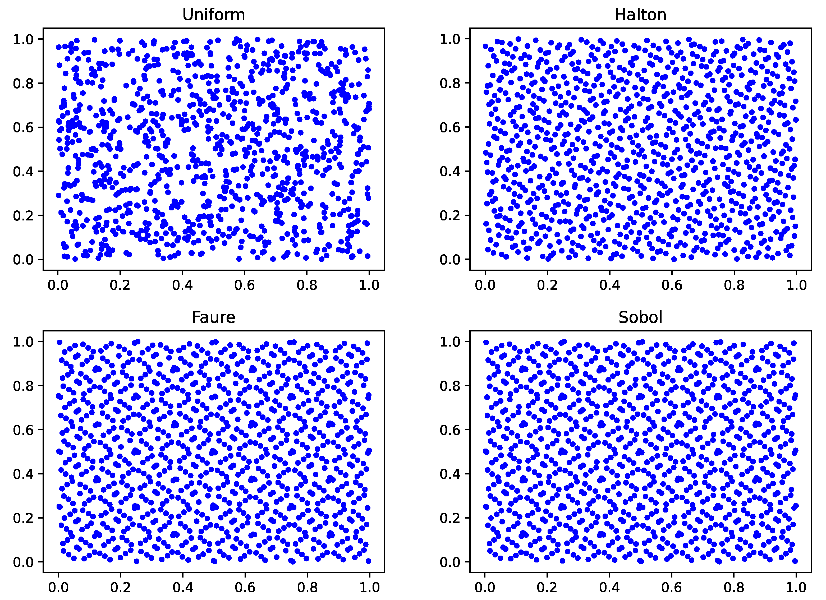
The Halton, Faure, and Sobol sequences are three commonly used low-discrepancy sequences. The generation of the Halton sequence depends on a prime number related to the dimension s. If the dimension , the smallest prime number 2 is taken as the number base. If the dimension , the second smallest prime number 3 is taken as the number base. Analogously, an s-dimensional Halton sequence would select the top s smallest prime numbers as the number base and then calculate the decimal decimals with the top s prime number as the base for any integer n. Meanwhile, the Faure sequence selects the smallest prime number greater than or equal to dimension s as the number base for each dimension. As a result, each dimensional sequence in the Faure sequence takes 2 as the number base and is a reordering of the first-dimensional sequence. Different from the Halton and Faure sequence, each dimension of the Sobol sequence consists of a radical inversion with base 2, but each dimension has a different matrix for the radical inversion. Due to each dimension taking 2 as the base, the Sobol sequence can be generated directly using bitwise operations to achieve radical inversion, which is very efficient.
To better demonstrate the difference between pseudo-random and low-discrepancy sequences, we randomly sampled 1000 points on a two-dimensional (first and second dimensions) space to observe their distributions. As shown in
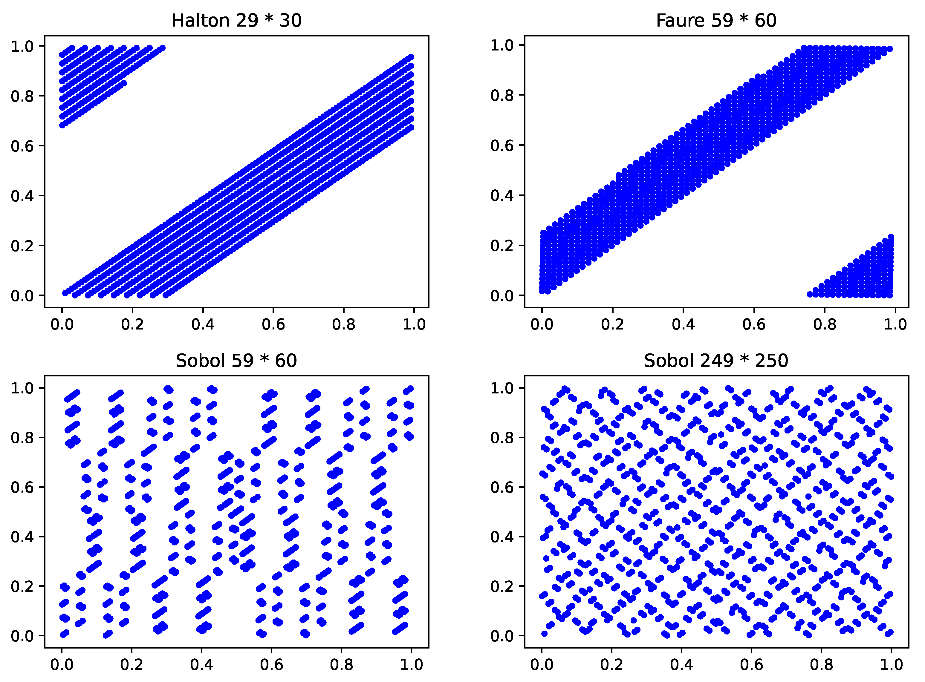
Figure 1, the Halton, Faure, and Sobol sequences are more evenly distributed than the pseudo-random sequence. In particular, we observe that the distribution of Faure and Sobol sequences in two-dimensional is the same, since they both take the prime 2 as the base, and the second dimension is a reordering of the data in the first dimension. It is worth noting that as the dimensionality increases, the low-discrepancy sequences degenerate to varying degrees. When the dimension is set to 30, the random data in the two adjacent dimensions (dimensions 29 and 30) of the Halton sequence show a high correlation, and the data are not evenly distributed in U[0, 1]. When the dimension is set to 60, the random data in the two adjacent dimensions (dimension 59 and 60) of the Faure sequence suffer from a similar problem. However, the Sobol sequence does not have this problem, and when the number of dimensions reaches 250, the data in the two adjacent dimensions (dimension 249 and 250) are still well distributed. Taking 1000 data points as examples, results in Halton, Faure and Sobol sequences can be seen in
Figure 2.
Furthermore, given that the fact that the Asian options are usually valid for 1 to 9 months, and the change in the price of the underlying asset is usually calculated in days, the pricing of Asian options is a high-dimensional problem (the dimension is usually greater than 30). Given that the Sobol sequence performs better in low-dimension and high-dimension scenarios, we choose the Sobol low-discrepancy sequence to generate random points for our numerical experiments. The construction details of the Sobol sequence can be seen in
Appendix A.
3.2.3. Inverse Transformation Algorithm
Notably, the above three low discrepancy sequences all obey the U[0, 1] distribution, but the B-S formula requires a normally distributed sequence, so it is necessary to convert the uniformly distributed sequences into standard normally distributed sequences. Although Box–Muller [
43,
44,
45] is the classical algorithm for solving this problem, it disturbs the uniformity of the low-discrepancy sequences. We will adopt the Moro algorithm [
46] for transformation. Since the value of the
Y-axis in the standard normal distribution obeys the U[0, 1] distribution, an intuitive idea is to inverse-normally transform the value of the
Y-axis. The Moro algorithm divides the
Y-axis of the standard normal distribution into two parts: the peak part (
) and the fat tail part (
and
).
The Moro algorithm uses different algorithms for different parts. Let y be a random number in the low-discrepancy sequence and .
If
, then we use the Beasley algorithm [
47] to calculate the estimate of the inverse function
If
, then we employ the truncated Chebyshev sequence to calculate the estimate of the inverse function
in which
, and the parameter value of
can be seen in
Appendix B.
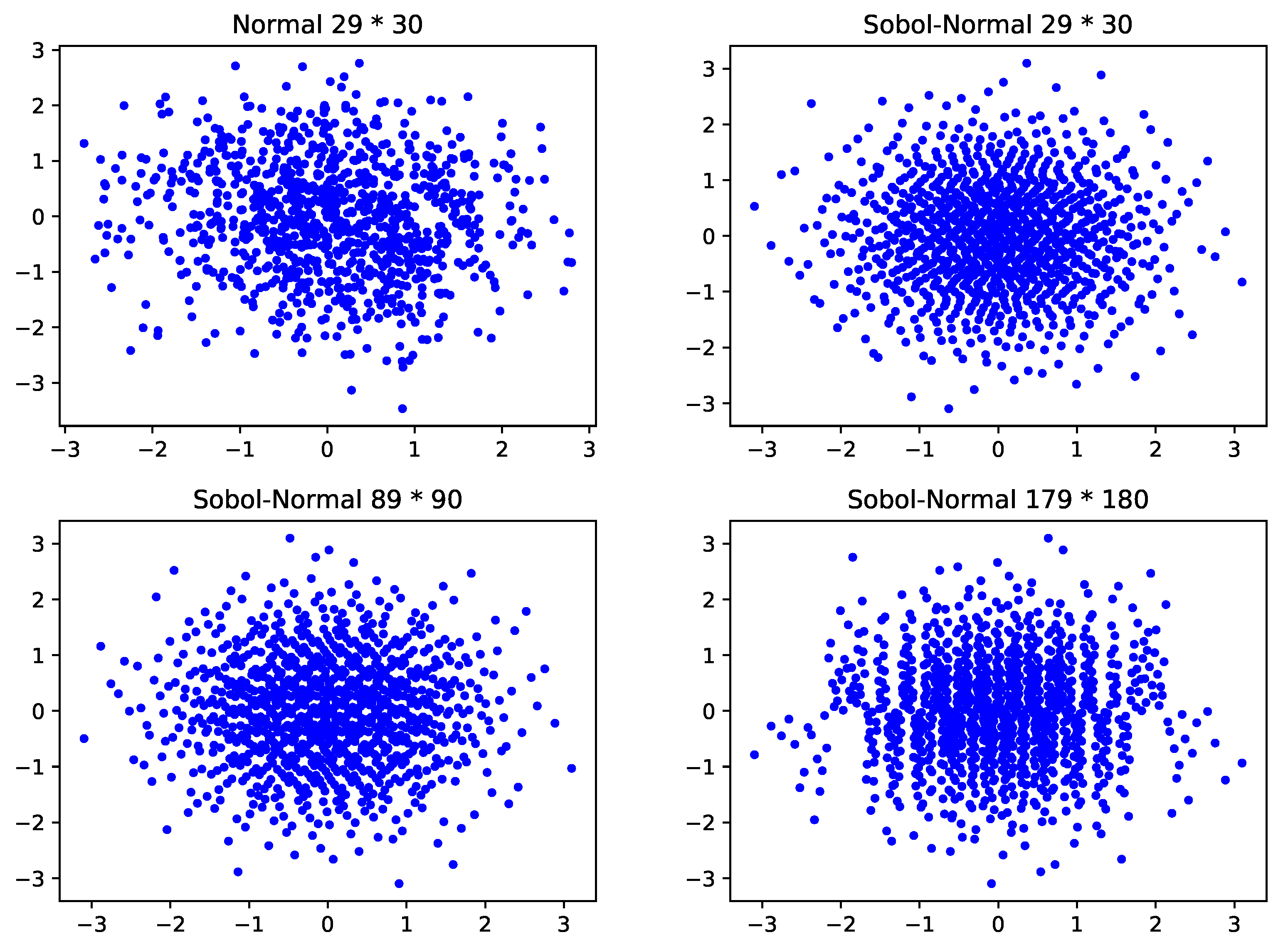
Next, we employ the Moro algorithm to transform the Sobol sequence into a normal distribution sequence. We consider the standard normal distribution for the two adjacent dimensions of 29 and 30, as well as the distribution of random data from the Sobol sequence in two adjacent dimensions after Moro normalization when the dimensions are set to 30, 90, and 180, respectively. As illustrated in
Figure 3, the normal distribution of the Moro-normalized Sobol sequence of adjacent two-dimensional data holds well as the number of dimensions increases.


