A Parametric Method Optimised for the Solution of the (2+1)-Dimensional Nonlinear Schrödinger Equation

Abstract

We investigate the numerical solution of the nonlinear Schrödinger equation in two spatial dimensions and one temporal dimension. We develop a parametric Runge–Kutta method with four of their coefficients considered as free parameters, and we provide the full process of constructing the method and the explicit formulas of all other coefficients. Consequently, we produce an adaptable method with four degrees of freedom, which permit further optimisation. In fact, with this methodology, we produce a family of methods, each of which can be tailored to a specific problem. We then optimise the new parametric method to obtain an optimal Runge–Kutta method that performs efficiently for the nonlinear Schrödinger equation. We perform a stability analysis, and utilise an exact dark soliton solution to measure the global error and mass error of the new method with and without the use of finite difference schemes for the spatial semi-discretisation. We also compare the efficiency of the new method and other numerical integrators, in terms of accuracy versus computational cost, revealing the superiority of the new method. The proposed methodology is general and can be applied to a variety of problems, without being limited to linear problems or problems with oscillatory/periodic solutions.

1. Introduction

We consider the (2+1)-dimensional nonlinear Schrödinger (NLS) equation of the form:

$$\begin{array}{c}i{u}_t+a{u}_{xx}+b{u}_{yy}+c{\left|u\right|}^{2}u+du=0,\hfill \\ u(x,y,t=0)=u_0(x,y),\hfill \end{array}$$

(1)

where $i=\sqrt{-1}$, $a,b,c,d\in \mathbb{R}$, $u(x,y,t):{\mathbb{R}}^3\to \mathbb{C}$ is a complex function of the spatial variables $x,y$ and the temporal variable t and $u_0(x,y):{\mathbb{R}}^2\to \mathbb{C}$. The term $i{u}_t$ denotes the temporal evolution, the terms $a{u}_{xx}$ and $b{u}_{yy}$ denote the dispersion with respect to x and y, respectively, while ${c\left|u\right|}^{2}u$ is a nonlinear term, whose introduction is motivated by several applications. Equation (1) can represent atomic Bose–Einstein condensates (BECs), in which case u expresses the mean-field function of the matter-wave, or, if applied in the context of nonlinear optics for the study of optical beams [1], u describes the complex electric field envelope, t is the propagation distance, and $x,y$ are the transverse coordinates [2,3].

The analytical solution of the NLS equation has attracted great interest in recent years, especially when the solutions are solitons [4,5,6,7]. Additionally, the numerical computation of the NLS equation is a critical part of the verification process of analytical theories. Different strategies have been adopted to solve the NLS equation, its linear counterpart, or differential equations with similar behaviour. A very significant factor in the efficiency of the computation lies in the time integrator; this is the case for both the scalar forms and vector forms after applying the method of lines. Preferred time integrators for the Schrödinger equation include Runge–Kutta(–Nyström) (RK/RKN) methods [8,9,10,11] and multistep methods [12,13,14,15]. RK/RKN methods are especially well-established, with various tools for achieving a high order of accuracy and obtaining intrinsic properties for specific problems, e.g., in [16,17], specialised RK methods were developed and optimised with differential evolution algorithms; in [18,19,20,21], RK/RKN methods were constructed for problems with periodic/oscillatory behaviour using fitting techniques; finally, in [22], a hybrid block method was produced for the efficient solution of differential systems. Many of the aforementioned techniques are targeted towards linear differential equations, ordinary differential equations, problems with oscillatory/periodic solutions or combinations of these. Here, we propose a general approach that can be applied to a problem without these limitations, and is tailored to a specific nonlinear partial differential equation that does not always exhibit periodic behaviour.

Following our previous work in [9], where we investigated the numerical solution of the NLS equation in (1+1) dimensions, here we extend this study to problems in (2+1) dimensions; that is, two dimensions in space and one in time. However, since this is a problem with increased significance that could be experimentally verified, we decided to follow a different approach and develop a method that is tailored to the efficient numerical solution of the problem. To achieve this, we initially developed a new parametric RK method, with as many coefficients as possible treated as free parameters. In this way, we produced an adaptable method with four degrees of freedom, which can be applied to a plethora of problems and specifically tailored to their efficient solution. Subsequently, in the case of problem (1), we selected the optimal values that correspond to the method with the minimum global error when integrating the problem for various step sizes. We chose to construct a method with six algebraic orders and eight stages, a maximised real stability interval, and coefficients with similar orders of magnitude, to minimise the round-off error.

The structure of this paper is as follows:

• In Section 2, we present the necessary theoretical concepts;
• In Section 3, we show the construction and analysis of the new RK method;
• In Section 4, we report the numerical experiments and results;
• In Section 5, we provide a discussion of the results and future perspectives;
• In Section 6, we communicate our conclusions.

2. Theory

2.1. Explicit Runge–Kutta Methods

For the numerical solution of Equation (1),

$$\begin{array}{c}\mathrm{let}(x,y,t)\in [x_L,x_R]\times [y_L,y_R]\times [0,t_R]\mathrm{and}\hfill \\ u_{l,m}^n\mathrm{denotes}\mathrm{an}\mathrm{approximation}\mathrm{of}u(x_l,y_m,t_n),\mathrm{where}\hfill \\ x_l=x_L+l\Delta x,l=0,1,\dots ,L-1,L=\frac{x_R-x_L}{\Delta x}+1,\Delta x>0,\hfill \\ y_m=y_L+m\Delta y,m=0,1,\dots ,M-1,M=\frac{y_R-y_L}{\Delta y}+1,\Delta y>0,\hfill \\ t_n=nh,n=0,1,\dots ,N-1,N=\frac{t_R}{h}+1,h>0.\hfill \end{array}$$

(2)

An $s–$stage explicit Runge–Kutta method for the solution of Equation (1) is presented below:

$$\left\{\begin{array}{c}{u}_{l,m}^{n+1}=u_{l,m}^n+h{\displaystyle \sum _{i=1}^s}{b}_i{k}_i\hfill \\ k_i=f(t_n+c_{i}h,u_{l,m}^n+h{\displaystyle \sum _{j=1}^{i-1}}{a}_{ij}{k}_j),i=1,\dots ,s\hfill \end{array}\right.or\begin{array}{cc}c& A\\ & b\end{array}$$

(3)

where $A=\left[a_{ij}\right]\in {\mathbb{R}}^{s\times s}$ is strictly lower triangular, $b={\left[b_i\right]}^T\in {\mathbb{R}}^s$, $c=\left[c_i\right]\in {\mathbb{R}}^s$, $a_{ij},b_i,c_i\in \mathbb{R}$, $i=1,2,\dots ,s$ and $j=1,2,\dots ,i-1$ are the coefficient matrices, $h=\Delta t$ is the step size in time, and f is defined in $u^{\prime }=f(x,y,t,u)$.

2.2. Algebraic Order Conditions

According to rooted tree analysis [23], there are 37 equations $(q_1-q_{37})$ that must be satisfied to obtain a Runge–Kutta method of sixth algebraic order and 7 additional equations for an explicit Runge–Kutta method with eight stages $(q_{38}-q_{44})$, with a total of 44 equations, as seen below in the set of Equation (4).

$$\begin{array}{c}{q}_1=be-1,q_2=bc-\frac{1}{2},q_3=b{c}^2-\frac{1}{3},q_4=bAc-\frac{1}{6},q_5=b{c}^3-\frac{1}{4},q_6=bCAc-\frac{1}{8},\hfill \\ q_7=bA{c}^2-\frac{1}{12},q_8=b{A}^{2}c-\frac{1}{24},q_9=b{c}^4-\frac{1}{5},q_{10}=b{C}^{2}Ac-\frac{1}{10},q_{11}=bCA{c}^2-\frac{1}{15},\hfill \\ q_{12}=bC{A}^{2}c-\frac{1}{30},q_{13}=bA{c}^3-\frac{1}{20},q_{14}=bACAc-\frac{1}{40},q_{15}=b{A}^2{c}^2-\frac{1}{60},\hfill \\ q_{16}=b{A}^{3}c-\frac{1}{120},q_{17}=b{\left(Ac\right)}^2-\frac{1}{20},q_{18}=b{c}^5-\frac{1}{6},q_{19}=b{C}^{3}Ac-\frac{1}{12},\hfill \\ q_{20}=b{C}^{2}A{c}^2-\frac{1}{18},q_{21}=bC{\left(Ac\right)}^2-\frac{1}{24},q_{22}=b{C}^2{A}^{2}c-\frac{1}{36},q_{23}=bCA{c}^3-\frac{1}{24},\hfill \\ q_{24}=bCACAc-\frac{1}{48},q_{25}=b\left(Ac\right)\ast \left(A{c}^2\right)-\frac{1}{36},q_{26}=bC{A}^{3}c-\frac{1}{144},q_{27}=b\left(Ac\right)\ast \left(A^{2}c\right)-\frac{1}{72},\hfill \\ q_{28}=bC{A}^2{c}^2-\frac{1}{72},q_{29}=bA{c}^4-\frac{1}{30},q_{30}=bA{C}^{2}Ac-\frac{1}{60},q_{31}=bACA{c}^2-\frac{1}{90},\hfill \\ q_{32}=bAC{A}^{2}c-\frac{1}{180},q_{33}=bA{\left(Ac\right)}^2-\frac{1}{120},q_{34}=b{A}^2{c}^3-\frac{1}{120},q_{35}=b{A}^{2}CAc-\frac{1}{240},\hfill \\ q_{36}=b{A}^3{c}^2-\frac{1}{360},q_{37}=b{A}^{4}c-\frac{1}{720},q_{i+36}={(Ae-c)}_i,\mathrm{where}i=2\left(1\right)8.\hfill \end{array}$$

(4)

Here, $e={[1,\dots ,1]}^T\in {\mathbb{R}}^s$, the diagonal matrix $C=diag\left(c\right)\in {\mathbb{R}}^{s\times s}$ has $C_{ii}=c_i$, $i=1,2,\dots ,s$, the operator * denotes element-wise multiplication and, finally, the powers of c, C and $Ac$ are defined as element-wise powers, i.e., $c^3=c\ast c\ast c$, whereas the powers of A are defined normally, i.e., $A^3=AAA$.

2.3. Stability

We consider the problem

$$u^{\prime }=i\omega u,u\left(0\right)=u_0\omega ,u_0\in \mathbb{R},$$

(5)

with exact solution $u\left(t\right)=u_0{e}^{i\omega t}$, which represents the circular orbit on the complex plane and $\omega$ its frequency.

Equation (5), solved numerically by the RK high-order method of Equation (3), yields the solution $u_m^{n+1}=R^n{u}_m^n$, where $R\left(v\right)=A_s\left(v^2\right)+iv{B}_s\left(v^2\right)$ is called the stability polynomial; $v=\omega h$ and $A_s,B_s$ are polynomials in $v^2$. The exact solution of Equation (5) satisfies the relation $\tilde{u}\left(t_{n+1}\right)=\tilde{u}\left(t_n\right)e^{i{v}_n}$. For a generic $v=v_n$, since $|e^{iv}|=1$ and $arg\left(e^{iv}\right)=v$ we have:

Definition 1. 

For the method of Equation (3), if $\left|R\right(v_R\left)\right|<1$ and $\left|R\right(v_R-ϵ\left)\right|>1$, for every $v\in I_R$ and every suitably small positive ϵ, then the real stability interval is $I_R=(v_R,0)$.

Definition 2. 

The stability region is defined as the set $S=\left\{z\in \mathbb{C}:\left|R\right(z\left)\right|<1\right\}$.

3. Construction and Analysis

3.1. Criteria

For the construction of the new method, we aimed to satisfy the following criteria:

• Parametric method with as many as possible coefficients treated as free parameters.
• Minimum global error when integrating problem (1) for various step sizes.
• Sixth algebraic order and eight stages, which implies 44 equations (4).
• Maximised real stability interval, based on Definition 2.
• Coefficients with similar orders of magnitude, to minimise the round-off error.

3.2. Parametric Method—General Case

We began the development by considering the 44 equations (4). There are 43 variables involved in these equations, and we fixed 10 of these, namely

$$c_3=\frac{1}{6},c_6=\frac{1}{2},c_8=1,b_2=0,b_3=0,a_{42}=0,a_{52}=0,a_{62}=0,a_{72}=0,a_{82}=0.$$

(6)

Of the remaining 33 variables, 29 are contained in $S_1=\left\{a_{21}\right.$, $a_{31}$, $a_{32}$, $a_{41}$, $a_{43}$, $a_{51}$, $a_{53}$, $a_{54}$, $a_{61}$, $a_{63}$, $a_{64}$, $a_{65}$, $a_{71}$, $a_{73}$, $a_{74}$, $a_{75}$, $a_{76}$, $a_{81}$, $a_{83}$, $a_{84}$, $a_{85}$, $a_{86}$, $a_{87}$, $b_1$, $b_4$, $b_5$, $b_6$, $b_7$, $\left.b_8\right\}$ and 4 are contained in $S_2=\left\{c_2,c_4,c_5,c_7\right\}$. We aimed to solve the system of 44 equations for the 29 variables in $S_1$, considering the 4 variables in $S_2$ as free parameters, thus effectively creating a general family of methods with 4 degrees of freedom. In order to solve the highly nonlinear system of equations, we used the mathematical software Maple. In Table 1 we solved the 29 equations in the specified order, solving for the variable mentioned after the equation. The order of equations and the selected variables are important, and were chosen so that the corresponding system after the variable substitution is the least complex. Otherwise, the system solution has impractical computation times.

Table 1. The order in which the equations are solved, followed by the variable for which each one is solved.

1. Solve $q_{38}$ for $a_{21}$	11. Solve $q_5$ for $b_5$	21. Solve $q_7$ for $a_{63}$
2. Solve $q_{39}$ for $a_{32}$	12. Solve $q_9$ for $b_4$	22. Solve $q_{12}$ for $a_{83}$
3. Solve $q_{40}$ for $a_{43}$	13. Solve $q_{18}$ for $b_1$	23. Solve $q_{27}$ for $a_{73}$
4. Solve $q_{41}$ for $a_{54}$	14. Solve $q_{10}$ for $a_{86}$	24. Solve $q_8$ for $a_{61}$
5. Solve $q_{42}$ for $a_{65}$	15. Solve $q_6$ for $a_{75}$	25. Solve $q_{23}$ for $a_{84}$
6. Solve $q_{43}$ for $a_{76}$	16. Solve $q_{19}$ for $a_{64}$	26. Solve $q_{13}$ for $a_{71}$
7. Solve $q_1$ for $b_8$	17. Solve $q_4$ for $a_{53}$	27. Solve $q_{29}$ for $a_{81}$
8. Solve $q_{44}$ for $a_{87}$	18. Solve $q_{21}$ for $a_{41}$	28. Solve $q_{28}$ for $a_{51}$
9. Solve $q_2$ for $b_7$	19. Solve $q_{20}$ for $a_{85}$	29. Solve $q_{26}$ for $a_{31}$
10. Solve $q_3$ for $b_6$	20. Solve $q_{11}$ for $a_{74}$

After solving the system of 29 equations, and due to our initial fixed values of 10 coefficients, all 44 equations are now satisfied, including the ones we did not explicitly solve. All coefficients, except for the initially fixed ones, now depend on $\left\{c_2,c_4,c_5,c_7\right\}$:

$$\begin{array}{c}{b}_1=\frac{10c_4{c}_5{c}_7-c_4-c_5-c_7+1}{60c_4{c}_5{c}_7}\hfill \\ b_4=\frac{c_5-1+c_7}{60\left(c_4-c_7\right)\left(-1+c_4\right)\left(c_4-c_5\right)\left(2c_4-1\right)c_4}\hfill \\ b_5=\frac{-c_4+1-c_7}{60\left(2c_5-1\right)c_5\left(c_5-c_7\right)\left(c_4-c_5\right)\left(c_5-1\right)}\hfill \\ b_6=\frac{\left(80\left(2c_7-1\right)c_5-40c_7+24\right)c_4+\left(-40c_7+24\right)c_5+24c_7-16}{15\left(2c_7-1\right)\left(2c_5-1\right)\left(2c_4-1\right)}\hfill \\ b_7=\frac{c_4+c_5-1}{\left(120c_7-60\right)\left(c_5-c_7\right)\left(c_4-c_7\right)c_7\left(-1+c_7\right)}\hfill \\ b_8=\frac{\left(\left(10c_7-10\right)c_5-10c_7+9\right)c_4+\left(-10c_7+9\right)c_5+9c_7-8}{60\left(c_7-1\right)\left(c_5-1\right)\left(-1+c_4\right)}\hfill \\ a_{21}=c_2\hfill \\ a_{31}=\frac{-1+12c_2}{72c_2}\hfill \\ a_{32}=\frac{1}{72c_2}\hfill \\ a_{41}=-3{c_4}^2+c_4\hfill \\ a_{43}=3{c_4}^2\hfill \\ a_{51}=-\frac{\left(30{c_4}^3{c}_5-10{c_4}^3-45{c_4}^2{c}_5+15c_4{c_5}^2+14{c_4}^2+6c_4{c}_5-4{c_5}^2-3c_4+c_5\right)c_5}{2c_4\left(5{c_4}^2-5c_4+1\right)}\hfill \\ a_{53}=\frac{90{c_4}^3{c_5}^2+\left(-150{c_5}^2+12c_5\right){c_4}^2+\left(45{c_5}^3+33{c_5}^2-3c_5\right)c_4-12{c_5}^3}{30{c_4}^3-35{c_4}^2+11c_4-1}\hfill \\ a_{54}=\frac{c_5\left(15c_4{c}_5-4c_4-4c_5+1\right)\left(c_4-c_5\right)}{60{c_4}^4-70{c_4}^3+22{c_4}^2-2c_4}\hfill \end{array}$$

(7)

$$\begin{array}{c}{a}_{61}=\frac{1}{48}\left(\left(\left(1200c_7-780\right){c_5}^2+\left(-900c_7+540\right)c_5+150c_7-90\right){c_4}^4+\left(\left(-2100c_7+1410\right){c_5}^2+\left(1590c_7-974\right)c_5-285c_7+175\right){c_4}^3+\right.\hfill \\ \left(\left(1380c_7-945\right){c_5}^2+\left(-1029c_7+645\right)c_5+195c_7-123\right){c_4}^2+\left(\left(-399c_7+279\right){c_5}^2+\left(291c_7-188\right)c_5-57c_7+37\right)c_4+\left(42c_7-30\right){c_5}^2+\hfill \\ \left.\left(-30c_7+20\right)c_5+6c_7-4\right){\left(c_5{c}_4\left(10c_4{c}_5{c}_7-5c_4{c}_5-5c_4{c}_7-5c_5{c}_7+3c_4+3c_5+3c_7-2\right)\left(5{c_4}^2-5c_4+1\right)\right)}^{-1}\hfill \\ a_{63}=\frac{180{c_4}^4{c}_5+\left(-300c_5+90c_7-66\right){c_4}^3+\left(\left(-90c_7+225\right)c_5-81c_7+63\right){c_4}^2+\left(\left(69c_7-87\right)c_5+15c_7-12\right)c_4-12\left(-1+c_7\right)c_5}{8\left(6c_4-1\right)\left(10c_4{c}_5{c}_7-5c_4{c}_5-5c_4{c}_7-5c_5{c}_7+3c_4+3c_5+3c_7-2\right)\left(5{c_4}^2-5c_4+1\right)}\hfill \\ a_{64}=-75\left(c_4-\frac{1}{2}\right)\left(\left(2c_4-2c_5\right)\left(10c_4{c}_5{c}_7-5c_4{c}_5-5c_4{c}_7-5c_5{c}_7+3c_4+3c_5+3c_7-2\right)\left(6c_4-1\right)c_4\left(5{c_4}^2-5c_4+1\right)\right.\hfill \\ \left(\left(\left(c_7-\frac{3}{5}\right){c_5}^2+\left(-\frac{9c_7}{10}+\frac{31}{60}\right)c_5+\frac{1}{5}{c}_7-\frac{3}{25}\right){c_4}^3+\left(\left(-\frac{7}{6}{c}_7+\frac{3}{4}\right){c_5}^2+\left(c_7-\frac{11}{18}\right)c_5-\frac{11c_7}{50}+\frac{5}{36}\right){c_4}^2\right.\hfill \\ {\left.\left.+\left(\left(\frac{5c_7}{12}-\frac{17}{60}\right){c_5}^2+\left(-\frac{33c_7}{100}+\frac{19}{90}\right)c_5+\frac{7c_7}{100}-\frac{41}{900}\right)c_4+\left(-\frac{7c_7}{150}+\frac{1}{30}\right){c_5}^2+\left(\frac{1}{30}{c}_7-\frac{1}{45}\right)c_5-\frac{c_7}{150}+\frac{1}{225}\right)\right)}^{-1}\hfill \\ a_{65}=\frac{\left(2c_5-1\right)\left(2c_4-1\right)\left(15c_4{c}_7-9c_4-6c_7+4\right)}{48c_5\left(10c_4{c}_5{c}_7-5c_4{c}_5-5c_4{c}_7-5c_5{c}_7+3c_4+3c_5+3c_7-2\right)\left(c_4-c_5\right)}\hfill \\ a_{71}=\frac{10c_7}{c_5\left({c_4}^2-c_4+\frac{1}{5}\right)\left(c_4+c_5-1\right)c_4}\left(\left(\left(\frac{2}{5}-c_5\right){c_7}^2+\left(-\frac{1}{4}+{c_5}^2+\frac{1}{10}{c}_5\right)c_7-\frac{4}{5}{c_5}^2+\frac{7c_5}{20}\right){c_4}^4+\left(\left(-\frac{2}{5}+c_5\right){c_7}^3+\left(-\frac{7}{20}-{c_5}^2+c_5\right){c_7}^2\right.\right.\hfill \\ \left.+\left(-\frac{9{c_5}^2}{10}-\frac{1}{10}{c}_5+\frac{23}{60}\right)c_7+\frac{13{c_5}^2}{10}-\frac{187c_5}{300}\right){c_4}^3+\left(\left(-\frac{7}{5}{c}_5+\frac{3}{5}\right){c_7}^3+\left(-\frac{31}{300}+\frac{7}{5}{c_5}^2-\frac{3c_5}{20}\right){c_7}^2+\left(\frac{23c_5}{150}-\frac{11}{60}-\frac{3{c_5}^2}{20}\right)c_7-\frac{7{c_5}^2}{10}+\frac{53c_5}{150}\right){c_4}^2\hfill \\ \left.+\left(\left(-\frac{7}{25}+\frac{3}{5}{c}_5\right){c_7}^3+\left(-\frac{c_5}{100}+\frac{43}{300}-\frac{3}{4}{c_5}^2\right){c_7}^2+\left(\frac{21{c_5}^2}{50}-\frac{13c_5}{75}+\frac{2}{75}\right)c_7+\frac{11{c_5}^2}{100}-\frac{17c_5}{300}\right)c_4+\frac{3c_7}{25}\left(\left(-\frac{2}{3}{c}_5+\frac{1}{3}\right){c_7}^2+\left({c_5}^2-\frac{2}{9}\right)c_7-\frac{3}{4}{c_5}^2+\frac{11c_5}{36}\right)\right)\hfill \\ a_{73}=\frac{90c_7}{\left(c_4+c_5-1\right)\left(6c_4-1\right)\left(5{c_4}^2-5c_4+1\right)}\left({c_4}^4{c}_5+\left({c_7}^2-\frac{5}{3}{c}_5-c_7+\frac{2}{15}\right){c_4}^3+\left(-\frac{7}{6}{c_7}^2+c_5+\frac{7}{6}{c}_7-\frac{1}{6}\right){c_4}^2+\left(\left(\frac{1}{2}{c}_5+\frac{7}{30}\right){c_7}^2\right.\right.\hfill \\ \left.\left.+\left(-\frac{1}{2}{c}_5-\frac{7}{30}\right)c_7-\frac{1}{6}{c}_5+\frac{1}{30}\right)c_4-\frac{2}{15}{c}_7\left(-1+c_7\right)c_5\right)\hfill \\ a_{74}=-\frac{300c_7\left(c_4-c_7\right)}{\left(2c_4-1\right)\left(c_4+c_5-1\right)\left(c_4-c_5\right)\left(6c_4-1\right)c_4\left(5{c_4}^2-5c_4+1\right)}\left(\left(\left(c_7-\frac{3}{5}\right){c_5}^2+\left(\frac{13}{60}+\frac{1}{5}{c}_7-{c_7}^2\right)c_5+\frac{2}{5}{c_7}^2+\frac{1}{75}-\frac{4c_7}{15}\right){c_4}^4\right.\hfill \\ +\left(\left(-\frac{47c_7}{30}+1\right){c_5}^2+\left(-\frac{1}{3}{c}_7+\frac{47{c_7}^2}{30}-\frac{133}{360}\right)c_5-\frac{2}{3}{c_7}^2+\frac{103c_7}{225}-\frac{7}{300}\right){c_4}^3+\left(\left(\frac{53c_7}{60}-\frac{3}{5}\right){c_5}^2+\left(\frac{47c_7}{300}-\frac{5}{6}{c_7}^2+\frac{139}{600}\right)c_5+\frac{19{c_7}^2}{50}-\frac{79c_7}{300}\right.\hfill \\ \left.\left.+\frac{7}{600}\right){c_4}^2+\left(\left(-\frac{131c_7}{600}+\frac{47}{300}\right){c_5}^2+\left(\frac{9{c_7}^2}{50}-\frac{13c_7}{600}-\frac{113}{1800}\right)c_5-\frac{1}{600}-\frac{13{c_7}^2}{150}+\frac{107c_7}{1800}\right)c_4+\left(-\frac{3}{200}+\frac{1}{50}{c}_7\right){c_5}^2+\left(\frac{11}{1800}-\frac{{c_7}^2}{75}\right)c_5+\frac{{c_7}^2}{150}-\frac{c_7}{225}\right)\hfill \\ a_{75}=\frac{c_7\left(c_5-c_7\right)\left(c_4-c_7\right)\left(60c_4{c}_5{c}_7-36c_4{c}_5-24c_4{c}_7-24c_5{c}_7+15c_4+16c_5+12c_7-8\right)}{12\left(c_5-\frac{1}{2}\right)c_5\left(c_4-c_5\right)\left(c_4+c_5-1\right)}\hfill \\ a_{76}=\frac{-4\left(2c_7-1\right)\left(c_5-c_7\right)\left(c_4-c_7\right)c_7\left(5c_4{c}_5-2c_4-2c_5+1\right)}{\left(2c_5-1\right)\left(2c_4-1\right)\left(c_4+c_5-1\right)}\hfill \\ a_{81}=\left(\left(\left(-300{c_5}^2+450c_5-150\right){c_7}^2+\left(240{c_5}^2-315c_5+135\right)c_7+30c_5-30\right){c_4}^4+\left(\left(750{c_5}^2-1080c_5+390\right){c_7}^2+\left(-600{c_5}^2+817c_5\right.\right.\right.\hfill \\ \left.\left.-370\right)c_7+30{c_5}^2-120c_5+90\right){c_4}^3+\left(\left(-705{c_5}^2+972c_5-360\right){c_7}^2+\left(600{c_5}^2-815c_5+362\right)c_7-60{c_5}^2+156c_5-96\right){c_4}^2+\left(\left(297{c_5}^2\right.\right.\hfill \\ \left.\left.\left.-381c_5+138\right){c_7}^2+\left(-267{c_5}^2+351c_5-147\right)c_7+36{c_5}^2-78c_5+42\right)c_4+\left(-42{c_5}^2+51c_5-18\right){c_7}^2+\left(39{c_5}^2-50c_5+20\right)c_7-6{\left(c_5-1\right)}^2\right)\hfill \\ {\left(300c_5{c}_7\left({c_4}^2-c_4+1/5\right)c_4\right)}^{-1}{\left(\left(\left(c_5-1\right)c_7-c_5+\frac{9}{10}\right)c_4+\left(-c_5+\frac{9}{10}\right)c_7+\frac{9c_5}{10}-4/5\right)}^{-1}\hfill \\ a_{83}=\frac{-90{c_4}^4{c}_5+\left(150c_5-90c_7+78\right){c_4}^3+\left(\left(45c_7-135\right)c_5+93c_7-78\right){c_4}^2+\left(\left(-57c_7+72\right)c_5-18c_7+15\right)c_4+12\left(-1+c_7\right)c_5}{\left(10c_4{c}_5{c}_7-10c_4{c}_5-10c_4{c}_7-10c_5{c}_7+9c_4+9c_5+9c_7-8\right)\left(6c_4-1\right)\left(5{c_4}^2-5c_4+1\right)}\hfill \\ a_{84}=300\left(-1+c_4\right){\left(\left(2c_4-1\right)\left(c_4-c_7\right)\left(c_4-c_5\right)\left(10c_4{c}_5{c}_7-10c_4{c}_5-10c_4{c}_7-10c_5{c}_7+9c_4+9c_5+9c_7-8\right)\left(6c_4-1\right)c_4\left(5{c_4}^2-5c_4+1\right)\right)}^{-1}\hfill \\ \left(\left(\left(c_7-\frac{3}{5}\right){c_5}^2+\left(\frac{49}{60}-\frac{7}{5}{c}_7\right)c_5+\frac{2}{5}{c}_7-\frac{19}{75}\right){c_4}^5+\left(\left(-{c_7}^2+\frac{11}{10}-\frac{16c_7}{15}\right){c_5}^2+\left(-\frac{511}{360}+\frac{22c_7}{15}+\frac{7}{5}{c_7}^2\right)c_5-\frac{2}{5}{c_7}^2+\frac{379}{900}-\frac{2}{5}{c}_7\right){c_4}^4\right.\hfill \\ +\left(\left(-\frac{1}{5}{c}_7+\frac{5}{3}{c_7}^2-\frac{37}{60}\right){c_5}^2+\left(\frac{373c_7}{900}-\frac{143{c_7}^2}{60}+\frac{33}{50}\right)c_5+\frac{113{c_7}^2}{150}-\frac{113c_7}{450}-\frac{17}{120}\right){c_4}^3+\left(\left(-{c_7}^2+\frac{347c_7}{600}+\frac{23}{300}\right){c_5}^2\right.\hfill \\ \left.+\left(-\frac{271c_7}{300}+\frac{853{c_7}^2}{600}+\frac{1}{45}\right)c_5-\frac{73{c_7}^2}{150}+\frac{39c_7}{100}-\frac{109}{1800}\right){c_4}^2+\left(\left(-\frac{31c_7}{150}+\frac{51{c_7}^2}{200}+\frac{11}{600}\right){c_5}^2+\left(-\frac{103{c_7}^2}{300}+\frac{533c_7}{1800}-\frac{1}{18}\right)c_5+\frac{29}{900}\right.\hfill \\ \left.\left.+\frac{73{c_7}^2}{600}-\frac{221c_7}{1800}\right)c_4+\left(-\frac{1}{300}-\frac{7{c_7}^2}{300}+\frac{13c_7}{600}\right){c_5}^2+\left(-\frac{1}{36}{c}_7+\frac{1}{150}+\frac{17{c_7}^2}{600}\right)c_5-\frac{{c_7}^2}{100}+\frac{c_7}{90}-\frac{1}{300}\right)\hfill \\ a_{85}=-\frac{\left(-1+c_4\right)\left(c_5-1\right)}{2\left(c_5-\frac{1}{2}\right)c_5\left(c_5-c_7\right)\left(c_4-c_5\right)}\left(\left(\left(c_4-\frac{2}{5}\right)c_7-\frac{3}{5}{c}_4+\frac{4}{15}\right){c_5}^2+\left(\left(-c_4+\frac{2}{5}\right){c_7}^2+\left(\frac{1}{10}{c}_4-\frac{1}{15}\right)c_7+\frac{7c_4}{20}-\frac{2}{15}\right)c_5+\left(\frac{1}{2}{c}_4-\frac{3}{10}\right){c_7}^2\right.\hfill \\ \left.+\left(-\frac{9c_4}{20}+\frac{1}{3}\right)c_7+\frac{1}{10}{c}_4-\frac{1}{10}\right){\left(\left(\left(-1+c_4\right)c_7-c_4+\frac{9}{10}\right)c_5+\left(-c_4+\frac{9}{10}\right)c_7+\frac{9c_4}{10}-\frac{4}{5}\right)}^{-1}\hfill \\ a_{86}=\frac{160\left(-1+c_4\right)\left(c_5-1\right)}{\left(2c_7-1\right)\left(10c_4{c}_5{c}_7-10c_4{c}_5-10c_4{c}_7-10c_5{c}_7+9c_4+9c_5+9c_7-8\right)\left(2c_5-1\right)\left(2c_4-1\right)}\left(\left(\left(c_5-\frac{1}{2}\right)c_4-\frac{1}{2}{c}_5+\frac{3}{10}\right){c_7}^2+\left(\left(-\frac{5}{4}{c}_5+\frac{7}{10}\right)c_4\right.\right.\hfill \\ \left.\left.+\frac{7c_5}{10}-\frac{9}{20}\right)c_7+\left(\frac{3}{8}{c}_5-\frac{1}{4}\right)c_4-\frac{1}{4}{c}_5+\frac{7}{40}\right)\hfill \\ a_{87}=-\frac{\left(c_5-1\right)\left(-1+c_4\right)\left(c_4+c_5-1\right)\left(-1+c_7\right)}{20\left(c_7-\frac{1}{2}\right)\left(c_5-c_7\right)\left(c_4-c_7\right)c_7}{\left(\left(\left(c_5-1\right)c_4-c_5+\frac{9}{10}\right)c_7+\left(-c_5+\frac{9}{10}\right)c_4+\frac{9c_5}{10}-\frac{4}{5}\right)}^{-1}\hfill \end{array}$$

(8)

3.3. Parametric Method—Optimal Case

After generating the parametric method, we aimed to identify the optimal method with the best performance. In order to achieve this, we selected different step-lengths and integrated problem (1). The optimal values of the four coefficients are considered the ones that yield higher accuracy results for all different step-lengths. The latter were chosen to be $\Delta t=\{0.1,0.04,0.01\}$, so that they can yield results with an accuracy of different orders of magnitudes. These step-lengths return results of above 4, 6.5 and 10 accurate decimal digits, respectively. These accuracy values were selected to be above average while still allowing for a plethora of feasible solutions/coefficient combinations, and will later be used as benchmarks. We are interested in the quadruples

$$(c_2,c_4,c_5,c_7),\mathrm{where}{c}_2,c_4,c_5,c_7\in [0,1],$$

for which the method has the highest accuracy. The optimisation process is as follows:

• We evaluate the accuracy at each grid point of the mesh defined by

  $$c_i=j\Delta c,i=\left\{2,4,5,7\right\},j=0,1,\dots ,C-1,C=\frac{1}{\Delta c}+1,\Delta c>0.$$
  In the first iteration, we choose the coefficient step-length $\Delta c=0.1$ and integration step-length $\Delta t=0.1$, and identify the regions with maximum accuracy. We observe that all high efficient quadruples appear to satisfy the constraint

  $$c_2\le c_4\le c_5\le c_7,$$

  as is also the case with the majority of RK methods. Thus, for the subsequent iterations, we impose this constraint in advance, which drastically reduces the computation cost without sacrificing the accuracy.
• For the next two iterations, we use $\Delta c=0.1$, together with $\Delta t=0.04$ and $\Delta t=0.01$, and follow the procedure of step 1. We identify the intersection of all regions for which a certain quadruple has a higher accuracy than its corresponding benchmark.
• We repeat this process for $\Delta c=0.01$ combined with $\Delta t=\{0.1,0.04,0.01\}$, as described in step 1, but only within the regions narrowed down by step 2, i.e.,

  $$(c_2,c_4,c_5,c_7)\in [0.01,0.16]\times [0.18,0.22]\times [0.31,0.45]\times [0.52,0.92].$$
• We run the process one last time for $\Delta c=0.001$ combined with $\Delta t=\{0.1,0.04,0.01\}$, within the regions updated by step 3, i.e.,

  $$(c_2,c_4,c_5,c_7)\in [0.001,0.010]\times [0.205,0.213]\times [0.435,0.445]\times [0.909,0.915].$$

The optimal quadruple is primarily chosen with respect to the accuracy, and secondarily considering the robustness of the solution. The latter is expressed by the absence of sensitivity of the solution when a coefficient value deviates from the optimal value. This is the reason why no further local optimisation is needed and why we stop at three decimal digits of accuracy for the optimal coefficient values.

The optimal values returned by the optimisation process are $\left\{c_2=0.007\right.$, $c_4=0.208$, $c_5=0.441$, $\left.c_7=0.915\right\}$. These can be exactly expressed as rational numbers $\left\{c_2=\frac{7}{1000}\right.$, $c_4=\frac{26}{125}$, $c_5=\frac{441}{1000}$, $\left.c_7=\frac{183}{200}\right\}$. By substituting these values to the other coefficients, we obtain the particular case that is optimal for this problem, as seen below in Table 2.

Table 2. The Butcher tableau of the optimised Runge–Kutta method.

$\frac{7}{1000}$	$\frac{7}{1000}$
$\frac{1}{6}$	$-\frac{229}{126}$	$\frac{125}{63}$
$\frac{26}{125}$	$\frac{1222}{15625}$	0	$\frac{2028}{15625}$
$\frac{441}{1000}$	$\frac{19009080531}{114608000000}$	0	$-\frac{66139404093}{68324000000}$	$\frac{282673503}{227382272}$
$\frac{1}{2}$	$\frac{498423839357}{3017837416104}$	0	$-\frac{33701852355}{35356371844}$	$\frac{60281311022875}{49428207837912}$	$\frac{10922552000}{159518175579}$
$\frac{183}{200}$	$-\frac{711091869877829}{844775568000000}$	0	$\frac{588657911761}{177642400000}$	$-\frac{37397696814038267}{56562846567552000}$	$-\frac{96981681064}{12666142125}$	$\frac{70978718489}{10498312500}$
1	$-\frac{144640010763881}{19166802690126}$	0	$\frac{61948580865}{2548536443}$	$-\frac{2761988623890181125}{796823971990899034}$	$-\frac{1484898545416000}{23819350452933}$	$\frac{2715651824886}{53337237643}$	$-\frac{36691083000000}{42192182210017}$
	$\frac{114713}{2098278}$	0	0	$\frac{17382812500}{46429926543}$	$-\frac{512500000000}{803168516241}$	$\frac{1034962}{1072443}$	$\frac{1300000000}{4807323563}$	$-\frac{149203}{5644782}$

3.4. Error and Stability Analysis

We perform local truncation error analysis on the method of Table 2, based on the Taylor expansion series of the difference

$$\epsilon =u_{l,m}^{n+1}-u(x_l,y_m,t_{n+1}).$$

The principal term of the local truncation error is evaluated as

$$\epsilon =\frac{227406522263}{6682354278516000}{u}^{\left(7\right)}\left(x\right)h^7,$$

which implies that while, locally, the order of accuracy is seven, globally, the order of the new method is six (see [23] for explanation).

Regarding the stability of the method, following the methodology of Section 2.3, we evaluated the stability polynomial of the method presented in Table 2. The polynomial is given by

$$R=1+z+\frac{1}{2}{z}^2+\frac{1}{6}{z}^3+\frac{1}{24}{z}^4+\frac{z^5}{120}+\frac{z^6}{720}+\frac{156922488841z^7}{954622039788000}+\frac{948518207z^8}{39775918324500}.$$

The stability analysis was carried out numerically in a mesh around the origin with $\Delta x=\Delta y=0.01$, and the stability region is shown in Figure 1, as the grid points that satisfy Definition 2. Furthermore, with a similar procedure performed on the real axis and according to Definition 1, the real stability interval is $\left(-3.99,0\right)$.

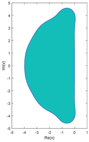
Figure 1. Stability region of the new Runge–Kutta method of Table 2.

4. Numerical Experiments

4.1. Theoretical Solution and Mass Conservation Law

Equation (1) has a dark soliton solution given by

$$u(x,y,t)=\sqrt{-\frac{\gamma }{c}}tanh\left(\sqrt{\frac{\gamma }{2\beta }}\left(k_{1}x+l_{1}y-2at+{\xi }_0\right)\right){\mathrm{e}}^{i\left(k_{2}x+l_{2}y-c_{2}t+{\eta }_0\right)}$$

(9)

where $\beta =a{k}_1^2+b{l}_1^2$ and $\gamma =c_2+d-ak{2}^2-b{l}_2^2$ [7]. We also choose, as in [7],

$$a=1,b=1,c=-1,d=1,k_1=1,k_2=1,l_1=0,l_2=0,c_2=2,{\xi }_0=0,{\eta }_0=0.$$

(10)

For this particular case, the theoretical solution becomes

$$u(x,y,t)=\sqrt{2}tanh\left(x-2t\right){\mathrm{e}}^{i\left(x-2t\right)}$$

(11)

and

$${\left|u(x,y,t)\right|}^2=2{\left|tanh\left(x-2t\right)\right|}^2,$$

which is called density.

Furthermore, the solution $u(x,y,t)$ of Equation (1) satisfies the mass conservation law [4]:

$$M\left[u\right]\left(t\right)=\underset{{\mathbb{R}}^2}{\int }{\left|u(x,y,t)\right|}^{2}dxdy\equiv M\left[u\right]\left(0\right).$$

(12)

4.2. Numerical Solution

We performed a numerical computation of problem (1), utilising the method of lines for $(x,y,t)\in [-20,30]\times [-1,1]\times [0,5]$. We used Equation (11) for both the initial condition and the boundary conditions. Regarding the semi-discretisation of $u_{xx}$ and $u_{yy}$, we chose a combination of 10th-order forward, central and backward finite difference schemes. Next, we defined the maximum absolute solution error and the maximum relative mass error of the numerical computation.

The maximum absolute solution error is given by

$$\underset{l,m,n}{max}\left(\right|u_{l,m}^n-u(x_l,y_m,t_n)\left|\right).$$

(13)

where $u_{l,m}^n$ denotes the numerical approximation of $u(x_l,y_m,t_n)$.

The maximum relative mass error over the region D is given by

$$\underset{n}{max}\left(\left|\frac{M_D^n-M_D^0}{M_D^0}\right|\right),$$

(14)

where $M_D^n$ is the numerical approximation of $M\left[u\right]\left(t_n\right)$ over the region $D=[-20,30]\times [-1,1]$ for $t\in [0,5]$, which provides a sufficiently constant density outside of it, as seen in Figure 2.

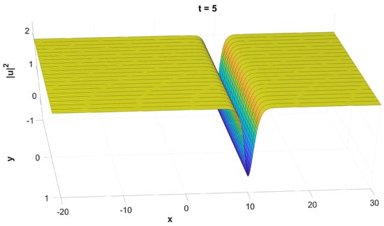
Figure 2. The graph of ${\left|u(x,y,t=5)\right|}^2$, evaluated numerically.

In Table 3, the maximum absolute solution error and the maximum relative mass error for different step sizes are shown. The $\Delta t$ is the maximum value that yields a stable solution for the preselected values of $\Delta x$ and $\Delta y$.

Table 3. The solution error and the mass relative error for different step sizes.

$\mathbf{\Delta }\mathit{x}$	$\mathbf{\Delta }\mathit{y}$	$\mathbf{\Delta }\mathit{t}$	Solution Error	Mass Error
0.5	0.5	0.14	$2.67$×${10}^{-3}$	$9.38\times {10}^{-6}$
0.2	0.2	0.024	$1.20\times {10}^{-6}$	$1.73\times {10}^{-9}$
0.1	0.1	0.006	$1.72\times {10}^{-9}$	$2.59\times {10}^{-12}$

In fact, the errors in Table 3 correspond to the total error of both the finite difference schemes for the semi-discretisation along x and y, and the integrator along time t. For the purpose of eliminating the semi-discretisation error and to analyse the performance of the time integrator alone, we used the second derivatives $u_{xx},u_{yy}$ of the solution (11) instead of applying the finite difference schemes. We used $\Delta x=\Delta y=0.1$ and $\Delta t=0.01$, and the results are presented in Figure 2, Figure 3, Figure 4, Figure 5, Figure 6 and Figure 7.

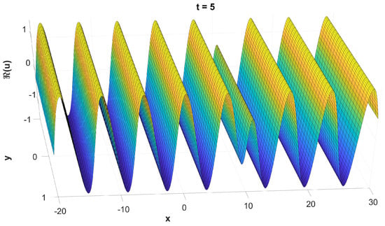
Figure 3. The graph of $\Re \left(u(x,y,t=5)\right)$, evaluated numerically.

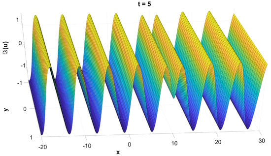
Figure 4. The graph of $\Im \left(u(x,y,t=5)\right)$, evaluated numerically.

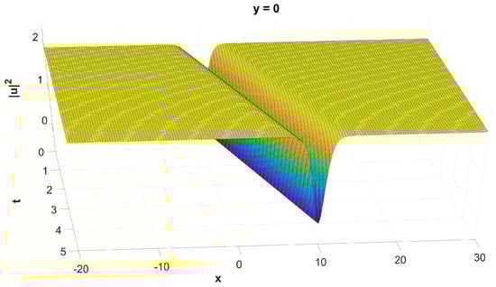
Figure 5. The graph of ${\left|u(x,y=0,t)\right|}^2$, evaluated numerically.

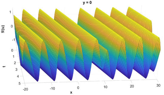
Figure 6. The graph of $\Re \left(u(x,y=0,t)\right)$, evaluated numerically.

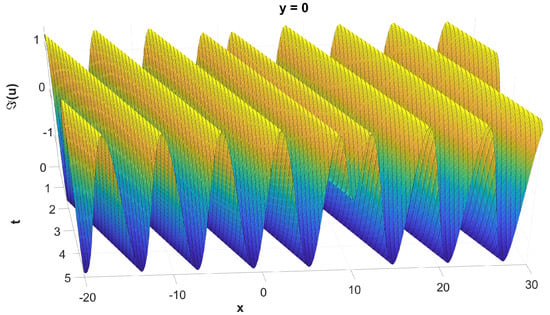
Figure 7. The graph of $\Im \left(u(x,y=0,t)\right)$, evaluated numerically.

The numerical solution of the dark soliton, namely, ${\left|u(x,y,t=5)\right|}^2$, $\Re \left(u(x,y,t=5)\right)$ and $\Im \left(u(x,y,t=5)\right)$ when solved by the new method of Table 2, are presented in Figure 2, Figure 3 and Figure 4 respectively. As expected from the physical properties of the dark soliton, this preserves its form while moving from $x=0$ (for $t=0$) to $x=10$ (for $t=5$).

Furthermore, we present the propagation of the dark soliton, namely ${\left|u(x,y=0,t)\right|}^2$, $\Re \left(u(x,y=0,t)\right)$ and $\Im \left(u(x,y=0,t)\right)$ when solved by the new method, in Figure 5, Figure 6 and Figure 7, respectively.

4.3. Error

We evaluated the error of the numerical approximation compared to the theoretical solution. We used two different implementations: in the first one, we used the second derivatives of the known solution and we chose $\Delta x=\Delta y=0.1$ and $\Delta t=0.01$; in the second one, we used finite difference schemes for the spatial semi-discretisation and we chose $\Delta x=\Delta y=0.1$ and $\Delta t=0.006$.

More specifically, we present

• The maximum, along $t_n\in [0,5]$, solution error ${\displaystyle \underset{n}{max}}\left(\right|u_{l,m}^n-u(x_l,y_m,t_n)\left|\right)$ without and with the use of finite difference schemes in Figure 8 and Figure 9, respectively;
  

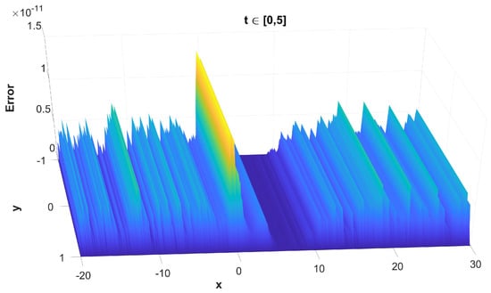  Figure 8. The maximum, along t, absolute error of the solution versus x and y without the use of finite difference schemes for the spatial semi-discretisation.
  

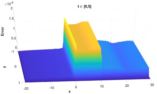  Figure 9. The maximum, along t, absolute error of the solution versus x and y with the use of finite difference schemes for the spatial semi-discretisation.
• The maximum, along $y_m\in [-1,1]$, solution error ${\displaystyle \underset{m}{max}}\left(\right|u_{l,m}^n-u(x_l,y_m,t_n)\left|\right)$ without and with the use of finite difference schemes in Figure 10 and Figure 11, respectively;
  

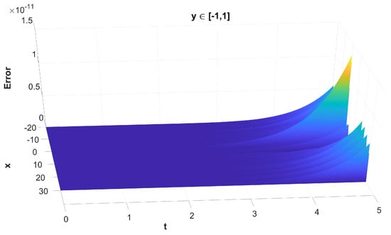  Figure 10. The maximum, along y, absolute error of the solution versus t and x without the use of finite difference schemes for the spatial semi-discretisation.
  

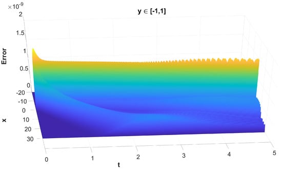  Figure 11. The maximum, along y, absolute error of the solution versus t and x with the use of finite difference schemes for the spatial semi-discretisation.
• The maximum, along $x_l\in [-20,30]$, solution error ${\displaystyle \underset{l}{max}}\left(\right|u_{l,m}^n-u(x_l,y_m,t_n)\left|\right)$ without and with the use of finite difference schemes in Figure 12 and Figure 13, respectively;
  

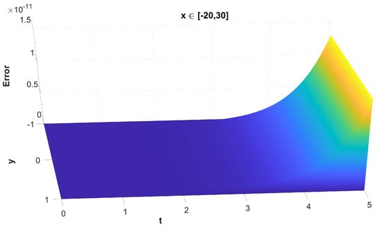  Figure 12. The maximum, along x, absolute error of the solution versus t and y without the use of finite difference schemes for the spatial semi-discretisation.
  

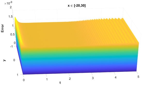  Figure 13. The maximum, along x, absolute error of the solution versus t and y with the use of finite difference schemes for the spatial semi-discretisation.
• The mass error $\frac{M_D^n-M_D^0}{M_D^0}$ versus $t_n=[0,5]$ without and with the use of finite difference schemes in Figure 14 and Figure 15 respectively.
  

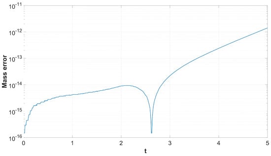  Figure 14. The mass error versus t without the use of finite difference schemes for the spatial semi-discretisation.
  

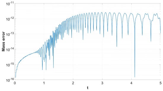  Figure 15. The mass error versus t with the use of finite difference schemes for the spatial semi-discretisation.

It is important to understand that, while Figure 8, Figure 10, Figure 12 and Figure 14 represent the error of the time-stepper alone, this is not the case for Figure 9, Figure 11, Figure 13 and Figure 15, where we observe the total error of the time-stepper in addition to the error of the space semi-discretisation finite difference scheme. Furthermore, the error of the finite difference scheme is dominant, and this is why the error in the second case is larger by approximately two orders of magnitude. We observe that, without the use of finite difference schemes for the spatial semi-discretisation, the maximum error is located near the area of the initial centre of the dark soliton $x=0$, without being propagated along with the dark soliton centre itself, as seen in Figure 8. However, with the use of finite difference schemes for spatial semi-discretisation, the error is propagated differently along x and y, as seen in Figure 9, mainly along the track of the soliton peak $x\in [0,10]$. Regarding the error propagation in time, the error without the finite difference schemes gradually increases, as seen in Figure 10 and Figure 12, while with the finite difference schemes it rapidly increases in the first time steps, then slightly decreases and stays at the same order of magnitude with small oscillations, as seen in Figure 11 and Figure 13. This is due to the effect of the space semi-discretisation scheme on the error, in combination with the time integrator. The oscillations are of a numerical nature and are a known phenomenon caused by the linear finite difference schemes applied in the spatial semi-discretisation. The same oscillations are also observed in the mass error with finite difference schemes, as seen in Figure 15, but are absent in Figure 14, where no finite difference schemes are applied.

4.4. Efficiency

We measured the efficiency of the new method with other methods from the literature and present the results in Figure 16 and Figure 17.

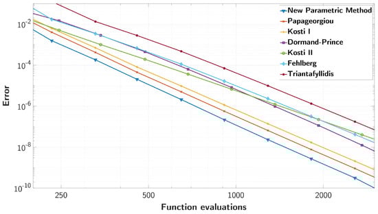
Figure 16. The maximum absolute error of the solution versus the function evaluations, for all compared methods.

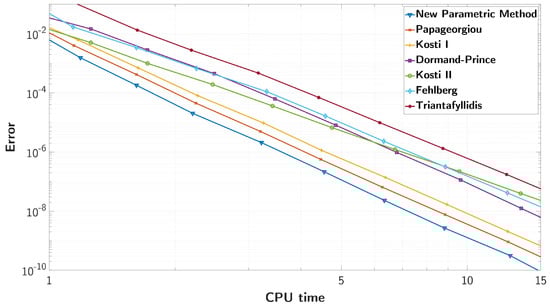
Figure 17. The maximum absolute error of the solution versus the CPU time, for all compared methods.

The compared methods are presented below:

• The new parametric method (Table 2)
• The method of Papageorgiou et al. [24]
• The method of Kosti et al. (I) [9]
• The method of Dormand et al. [23]
• The method of Kosti et al. (II) [10]
• The method of Fehlberg et al. [23]
• The method of Triantafyllidis et al. [11]

The efficiency of all compared methods in terms of the maximum absolute solution error, as expressed by (13), versus the function evaluations is presented in Figure 16. The order of accuracy of each method is represented by the slope of its corresponding efficiency line. Indeed, we verify that, except for two methods with fifth order and, thus, a smaller slope, five methods have sixth order, for which the lines are almost parallel. Additionally, we present the maximum absolute solution error versus the CPU time in seconds in Figure 17. In order to avoid fluctuations, we repeated each solution 10 times and used the median CPU time. We observe that the two graphs are similar, as the main contributor to the total computation time is the function evaluations. Furthermore, we see that the new optimised method is more efficient than all the other methods for all error orders.

5. Discussion

The numerical results are robust, exhibiting high efficiency among all step size values, with and without the use of finite difference schemes for the spatial semi-discretisation. Furthermore, the error propagation in time is typical of other explicit RK methods. The time integrator error is better showcased when no finite difference schemes are used, as in the case with finite difference schemes the error of the spatial discretisation method is dominant.

In general, the development of new RK methods that are more efficient than established methods in the literature is a challenging task, as one step of the method construction involves the solution of a system of numerous highly nonlinear equations. This is especially true for high-order methods that require a high number of stages, where the only way to solve the system is to use simplifying assumptions and/or fixed values for a set of coefficients. To our knowledge, there have been no explicit RK methods with order six or higher produced without the use of pre-determined coefficient values or simplifying assumptions. The solution with hand calculations is impossible, even for methods that use some assumptions, and even when using computer algebra software, as the solution is limited by the available computer memory and computational power. Leaving some variables free until the end of the system solution increases the complexity even further, but allows for the parameterisation of the method. Here, we managed to find a combination of a minimum number of fixed coefficients that still yields a solution with four free coefficients. The latter provide the method with some adaptability due to the four degrees of freedom. This versatility permits further optimisation, allowing for the construction of a method tailored to the nonlinear Schrödinger equation. The proposed methodology is general and can be applied to many problems, without being limited to linear problems or problems with oscillatory/periodic solutions.

Although the methodology offers satisfactory results, it also has limitations, namely the need to manually select the initially fixed coefficients and, most importantly, the actual fixed coefficients themselves, which hinder the optimisation potential of the method’s accuracy. Ideally, we aim to develop an optimisation process that concurrently maximises the number of free coefficients, minimises the number of fixed coefficients, and leads to a solvable system. Additionally, in our future work, we could combine this technique with other established techniques for better results, e.g., fitting techniques for problems with periodic solutions.

6. Conclusions

In this paper, we investigated the numerical solution of the (2+1)-dimensional nonlinear Schrödinger equation. We developed a parametric sixth-order eight-stage explicit Runge–Kutta method with four of their coefficients treated as free parameters/degrees of freedom, and we provided the full process of constructing the method and the explicit formulas of all other coefficients. We optimised the new parametric method to obtain the optimal Runge–Kutta method that performs efficiently by numerical testing. We performed stability analysis, and we utilised an exact dark soliton solution to measure the global error and the mass error of the new method. We also compared the efficiency of the new method and other numerical integrators, revealing the superiority of the new method.

References

- Moloney, J.V.; Newell, A.C. Nonlinear optics. Phys. D Nonlinear Phenom. 1990, 44, 1–37. [Google Scholar] [CrossRef]
- Pitaevskii, L.; Stringari, S. Bose-Einstein Condensation; Oxford University Press: Oxford, UK, 2003. [Google Scholar]
- Malomed, B. Multi-Component Bose-Einstein Condensates: Theory. In Emergent Nonlinear Phenomena in Bose-Einstein Condensates: Theory and Experiment; Springer: Berlin/Heidelberg, Germany, 2008; pp. 287–305. [Google Scholar] [CrossRef]
- Guardia, M.; Hani, Z.; Haus, E.; Maspero, A.; Procesi, M. Strong nonlinear instability and growth of Sobolev norms near quasiperiodic finite gap tori for the 2D cubic NLS equation. J. Eur. Math. Soc. 2022. published online first. [Google Scholar] [CrossRef]
- Tsitoura, F.; Anastassi, Z.A.; Marzuola, J.L.; Kevrekidis, P.G.; Frantzeskakis, D.J. Dark Solitons Potential Nonlinearity Steps. Phys. Rev. A 2016, 94, 063612. [Google Scholar] [CrossRef]
- Tsitoura, F.; Anastassi, Z.A.; Marzuola, J.L.; Kevrekidis, P.G.; Frantzeskakis, D.J. Dark soliton scattering in symmetric and asymmetric double potential barriers. Phys. Lett. A 2017, 381, 2514–2520. [Google Scholar] [CrossRef]
- Feng, D.; Jiao, J.; Jiang, G. Optical solitons and periodic solutions of the (2+1)-dimensional nonlinear Schrödinger’s equation. Phys. Lett. A 2018, 382, 2081–2084. [Google Scholar] [CrossRef]
- Fang, Y.; Yang, Y.; You, X.; Ma, L. Modified THDRK methods for the numerical integration of the Schrödinger equation. Int. J. Mod. Phys. C 2020, 31, 2050149. [Google Scholar] [CrossRef]
- Kosti, A.A.; Colreavy-Donnelly, S.; Caraffini, F.; Anastassi, Z.A. Efficient Computation of the Nonlinear Schrödinger Equation with Time-Dependent Coefficients. Mathematics 2020, 8, 374. [Google Scholar] [CrossRef]
- Kosti, A.A.; Anastassi, Z.A.; Simos, T.E. An optimized explicit Runge–Kutta method with increased phase-lag order for the numerical solution of the Schrödinger equation and related problems. J. Math. Chem. 2010, 47, 315. [Google Scholar] [CrossRef]
- Triantafyllidis, T.V.; Anastassi, Z.A.; Simos, T.E. Two optimized Runge–Kutta methods for the solution of the Schrödinger equation. MATCH Commun. Math. Comput. Chem. 2008, 60, 3. [Google Scholar]
- Zhang, Y.; Fang, Y.; You, X.; Liu, G. Trigonometrically-fitted multi-derivative linear methods for the resonant state of the Schrödinger equation. J. Math. Chem. 2018, 56, 1250–1261. [Google Scholar] [CrossRef]
- Shokri, A.; Mehdizadeh Khalsaraei, M. A new implicit high-order six-step singularly P-stable method for the numerical solution of Schrödinger equation. J. Math. Chem. 2021, 59, 224–249. [Google Scholar] [CrossRef]
- Shokri, A.; Vigo-Aguiar, J.; Mehdizadeh Khalsaraei, M.; Garcia-Rubio, R. A new implicit six-step P-stable method for the numerical solution of Schrödinger equation. J. Math. Chem. 2019, 97, 802–817. [Google Scholar] [CrossRef]
- Obaidat, S.; Mesloub, S. A New Explicit Four-Step Symmetric Method for Solving Schrödinger’s Equation. Mathematics 2019, 7, 1124. [Google Scholar] [CrossRef]
- Jerbi, H.; Ben Aoun, S.; Omri, M.; Simos, T.E.; Tsitouras, C. A Neural Network Type Approach for Constructing Runge–Kutta Pairs of Orders Six and Five That Perform Best on Problems with Oscillatory Solutions. Mathematics 2022, 10, 827. [Google Scholar] [CrossRef]
- Kovalnogov, V.N.; Fedorov, R.V.; Khakhalev, Y.A.; Simos, T.E.; Tsitouras, C. A Neural Network Technique for the Derivation of Runge–Kutta Pairs Adjusted for Scalar Autonomous Problems. Mathematics 2021, 9, 1842. [Google Scholar] [CrossRef]
- Anastassi, Z.A.; Kosti, A.A. A 6(4) optimized embedded Runge–Kutta–Nyström pair for the numerical solution of periodic problems. J. Comput. Appl. Math. 2015, 275, 311–320. [Google Scholar] [CrossRef]
- Kosti, A.A.; Anastassi, Z.A. Explicit almost P-stable Runge–Kutta–Nyström methods for the numerical solution of the two-body problem. Comput. Appl. Math. 2015, 34, 647–659. [Google Scholar] [CrossRef]
- Demba, M.; Senu, N.; Ismail, F. A 5(4) Embedded Pair of Explicit Trigonometrically-Fitted Runge–Kutta–Nyström Methods for the Numerical Solution of Oscillatory Initial Value Problems. Math. Comput. Appl. 2016, 21, 46. [Google Scholar] [CrossRef]
- Ahmad, N.A.; Senu, N.; Ismail, F. Phase-Fitted and Amplification-Fitted Higher Order Two-Derivative Runge–Kutta Method for the Numerical Solution of Orbital and Related Periodical IVPs. Math. Probl. Eng. 2017, 2017, 1871278. [Google Scholar] [CrossRef]
- Ramos, H.; Rufai, M.A. An adaptive one-point second-derivative Lobatto-type hybrid method for solving efficiently differential systems. Int. J. Comput. Math. 2022, 99, 1687–1705. [Google Scholar] [CrossRef]
- Butcher, J.C. Trees and numerical methods for ordinary differential equations. Numer. Alg. 2010, 53, 153–170. [Google Scholar] [CrossRef]
- Papageorgiou, G.; Tsitouras, C.; Papakostas, S.N. Runge-Kutta pairs for periodic initial value problems. Computing 1993, 51, 151–163. [Google Scholar] [CrossRef]
Disclaimer/Publisher’s Note: The statements, opinions and data contained in all publications are solely those of the individual author(s) and contributor(s) and not of MDPI and/or the editor(s). MDPI and/or the editor(s) disclaim responsibility for any injury to people or property resulting from any ideas, methods, instructions or products referred to in the content. |
© 2023 by the authors. Licensee MDPI, Basel, Switzerland. This article is an open access article distributed under the terms and conditions of the Creative Commons Attribution (CC BY) license (https://creativecommons.org/licenses/by/4.0/).