A New Method for Free Vibration Analysis of Triangular Isotropic and Orthotropic Plates of Isosceles Type Using an Accurate Series Solution

Abstract

In this paper, a new method based on an accurate analytical series solution for free vibration of triangular isotropic and orthotropic plates is presented. The proposed solution is expressed in terms of undetermined arbitrary coefficients, which are exactly satisfied by the governing differential equation in free vibration. The approach used is based on an innovative extension of the superposition method through the application of a modified system of trigonometric functions. The boundary conditions for bending displacements and bending rotations on the sides of the triangular plate led to an infinite system of linear algebraic equations in terms of the undetermined coefficients. Following this development, the paper then presents an algorithm to solve the boundary value problem for isotropic and orthotropic triangular plates for any kinematic boundary conditions. Of course, the boundary conditions with zero displacements and zero rotations on all sides correspond to the case when the plate is fully clamped all around. The convergence of the proposed method is examined by numerical simulation applying stringent accuracy requirements to fulfill the prescribed boundary conditions. Some of the computed numerical results are compared with published results and finally, the paper draws significant conclusions.

1. Introduction

The problem of free vibration of triangular plates has always been a more challenging problem than that of the relatively simpler problem of rectangular plates, for which the level of complexity is certainly less. Engineering structures of triangular shapes can be found in a wide range of practical applications, but importantly, triangular plate elements can be successfully used as building blocks to model complex structures accurately, particularly when applying the finite element method (FEM). Despite the importance of the problem and the underlying need for its investigation, the first publication with good coverage on the free vibration of triangular plates appeared only in the second half of the 20th century. The monograph published by Leissa [1] pointed out that in contrast to a rectangular plate, the variables in the skew coordinate system as generally encountered in a triangular plate are problematic and cannot be easily separated, thus making it difficult to obtain the general solution of the governing differential equation in series form. This could probably be the main reason why the earlier investigators used a variety of variational methods to solve the problem of vibration of triangular plates [2,3,4,5]. The superposition method developed by Gorman [6] for the analysis of the free vibration of rectangular plates based on exact solutions of the governing differential equations in free vibration is known to be one of the most accurate and reliable approaches to addressing the plate vibration problem. This method was later generalized by Gorman himself [7,8,9] to deal with the free vibration problem of right triangular plates, particularly when the edges of the plate are simply supported or clamped [7,8]. He also proposed, in another paper [9], an analytical solution for the right triangular plate for different boundary conditions with one of the edges of the plate free. It should be noted that the approach presented by Gorman is in many ways unique because the solution satisfies the governing differential equation a priori.

Kim and Dickinson [10,11] investigated the flexural vibration of isotropic and orthotropic triangular plates based on the Rayleigh–Ritz method, whereas Singh and Chakraverty [12] proposed the use of orthogonal polynomials in two variables as the basis function when applying the Rayleigh–Ritz method to arrive at the solution. A modification of the approach used in [12] can be found in the work of Pradhan and Chakraverty [13]. Based on a variational approach, Leissa and Jabber [14] investigated the free vibration behavior of triangular plates with completely free edges. A different analytical approach based on Green’s function was presented by Irie et al. [15] when they studied the fee vibration problem of isotropic polygonal plates, including triangular ones. Unfortunately, the convergence of the method they proposed in [15] is slow to achieve sufficiently accurate and reliable results, and rather unfavorably, their investigation revealed that for triangular plates, one must take up to 80 terms in the representation of Green’s function to attain acceptable accuracy. Sakiyama and Huang [16] also used Green’s function method to solve the free vibration problem of right triangular plates. Interestingly, a numerical method based on a hybrid form of the Rayleigh–Ritz method together with the Lagrangian multiplier method was reported by Liew and Wang [17] for free vibration analysis of triangular plates with point supports, mixed edges, as well as with some partial internal curved supports. The free vibration of point-supported isotropic and symmetrically laminated composite triangular plates has also been investigated by Abrate [18] with the help of the modified Rayleigh–Ritz method. By contrast, Haldar et al. [19] proposed an FEM approach based on high-precision triangular plate bending elements for free vibration analysis of laminated thick composite triangular plates. Pertinently, the free vibration analysis of isosceles triangular thick plates using the Ritz method was carried out by Cheung and Zhou [20], amongst others. Zhang and Li [21] presented a hybrid solution method for free vibration analysis of arbitrarily shaped triangular plates with elastically restrained edges.

A review of recent articles which are devoted to free vibration analysis of triangular plates shows that investigations in this area are predominantly based on the Rayleigh–Ritz method or in some forms of its modifications. For instance, Lv and Shi [22] used the Rayleigh–Ritz method through the application of modified Fourier series for free vibration analysis of arbitrarily shaped laminated triangular thin plates with elastic boundary conditions. Wang et al. [23] utilized a similar method for free vibration analysis of moderately thick composite triangular plates under multi-points support boundary conditions. On the other hand, the effect of thermal gradient on the free vibration of a bidirectional tapered triangular plate was investigated by Kaur and Khanna [24]. Free vibration analysis of thin arbitrary-shaped triangular plates under various boundary conditions and internal supports was carried out by Cai et al. [25], whereas a semi-analytical method for the free transverse vibration of polygonal isotropic thin plates with arbitrary shapes and elastically restrained edges was promoted by Zhao et al. [26], who essentially used the Rayleigh–Ritz method.

In the early seventies, Wittrick and Williams developed the dynamic stiffness method (DSM) [27], and its solution technique [28], known as the Wittrick–Williams algorithm. Following their pioneering contributions, the DSM has now proved to be a powerful and elegant tool in free vibration analysis and no doubt an efficient alternative to FEM. In their original paper, Wittrick and Williams [27] considered the case of free vibration analysis of rectangular plates when the two opposite sides of the plate are simply supported. In subsequent years, the area of applications of the DSM significantly expanded [29,30,31,32,33,34,35,36], including thin-walled structures, multilayer plates, beam structures, and shells, amongst others. The DSM uses an exact solution of governing differential equations of motion in free vibration of a structural element to describe the deformed shape or the shape function of the structural element. The building block in DSM is the single frequency-dependent element matrix which contains both the mass and stiffness properties of the element, which is in sharp contrast to FEM, which uses separate frequency-independent mass and stiffness matrices. The rest of the procedures in DSM, such as the assembly method using coordinate transformation to form the overall dynamic matrix of the final structure, are similar to that of the FEM, but the solution technique in DSM is different from the FEM. This is because the DSM leads to a non-linear eigenvalue problem for which the Wittrick–Williams algorithm [28] is customarily used to compute the natural frequencies, whereas the FEM generally leads to a linear eigenvalue problem. It should be noted that the main problem that arises in the development of DSM is the construction of the dynamic stiffness matrix of a structural element, which relates the boundary forces to boundary displacements of the element. For plate vibration problems, the original work of Wittrick and Williams [27], which was restricted to simply supported rectangular plates, has been significantly advanced in recent years by Banerjee et al. [35] and Papkov and Banerjee [36], amongst others to cover general cases involving all possible boundary conditions. However, there does not seem to be any attempt made so far to develop the DSM for triangular plate elements and, understandably, the task appeared to be too daunting. It is clear from previous DSM investigations that obtaining the general solution of the governing differential equation of a structural element in free vibration and imposing appropriate boundary conditions are the essential preliminary steps and undoubtedly the fundamental prerequisites towards developing the dynamic stiffness matrix of the element. Such an endeavor does not give the dynamic stiffness matrix straightaway because significant additional efforts are needed to relate the amplitudes of forces to those of the displacements at the boundaries of the element, but nevertheless, it prepares the necessary background for its dynamic stiffness matrix development. Thus, to investigate the free vibration behavior of a single structural element for different boundary conditions, the proposed endeavor is ideally suited and without doubt a significant step forward to dynamic stiffness matrix development. Within this pretext, this paper gives an accurate method based on the closed-form analytical solution for free vibration of isosceles triangular isotropic and orthotropic plates, paving the way for the development of its dynamic stiffness matrix. Representative results for natural frequencies and mode shapes for isotropic and orthotropic triangular plates are presented and some results are compared with published results. The paper closes by drawing significant conclusions.

2. Theory Formulation

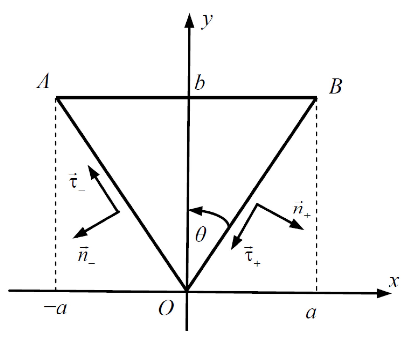
2.1. Governing Differential Equation and Boundary Value Problem

Let us consider the free transverse or bending vibration of a uniform isosceles triangular orthotropic plate (see Figure 1). Application of the classical Kirchhoff–Love theory of a thin orthotropic plate in free transverse or bending vibration leads to the following governing differential equation for the bending displacement $w^0(x,y,t)=W(x,y)e^{i\omega t}$, as described in [1].

$$D_1\frac{{\partial }^{4}W}{\partial x^4}+2D_3\frac{{\partial }^{4}W}{\partial x^2\partial y^2}+D_2\frac{{\partial }^{4}W}{\partial y^4}-{\mathsf{\Omega }}^{4}W=0$$

(1)

where W is the amplitude of the bending displacement, ω is the circular or angular frequency in rad/s, h is the thickness, ρ is the mass density of the plate, and $D_1,D_2,D_3$ are given by:

$$D_1=\frac{E_1{h}^3}{12(1-{\nu }_{12}{\nu }_{21})};\hspace{0.17em}{D}_2=\frac{E_2{h}^3}{12(1-{\nu }_{12}{\nu }_{21})};\hspace{0.17em}{D}_3=\frac{{\nu }_{12}{E}_2{h}^3}{12(1-{\nu }_{12}{\nu }_{21})}+\frac{G_{12}{h}^3}{6}$$

(2)

where E₁, E₂, G₁₂, and υ₁₂ (or υ₂₁) are the usual elastic constants and major and minor Poisson’s ratio of the orthotropic plate and ${\mathsf{\Omega }}^4={\omega }^2\rho h$ is the usual frequency parameter generally used in the analysis. Note that Ω⁴ is not a non-dimensional quantity and Equation (1) applies to any plate of any shape and size with thickness h, but for presentational purposes of results in the particular context of the present paper dealing with isosceles triangular plate, Ω is non-dimensionalized to $\overline{\mathsf{\Omega }}$ by introducing b, which is one of the sides of the isosceles triangle (AB) shown in Figure 1 to give ${\overline{\mathsf{\Omega }}}^4=b^4{\mathsf{\Omega }}^4/D_1$.

In order to write the boundary conditions on the sides of the triangle, OA and OB (see Figure 1), we introduce the following normal vectors:

$${\overrightarrow{n}}_{-}\left(-\cos \theta ;-\sin \theta \right);{\overrightarrow{n}}_{+}\left(\cos \theta ;-\sin \theta \right)$$

(3)

where, as shown in Figure 1, the angle θ connects the sides a and b of the triangle so that:

$$\theta =\arcsin \frac{a}{\sqrt{a^2+b^2}}$$

(4)

The boundary conditions for the amplitudes of bending displacement and the bending rotation of the plate cross-section on the side AB of the triangular plate of Figure 1, i.e., at (y = b, $x\in \left[-a;a\right]$), can be written as:

$$W=W_{AB}\left(x\right)$$

(5)

$$\frac{\partial W}{\partial y}={\mathsf{\varphi }}_{AB}\left(x\right)$$

(6)

Likewise, on the sides OB and OA of the triangular plate, i.e., at $x=\pm ky, y\in [0;b]$, where $k=\tan \theta$, can be written as follows:

$$W=W_{n\pm }\left(y\right)$$

(7)

$$\frac{\partial W}{\partial n_{\pm }}={\mathsf{\varphi }}_{n\pm }\left(y\right)$$

(8)

Now, let the functions on the right-hand sides of Equations (5)–(8) have the following trigonometric expansions:

$$W_{AB}\left(x\right)={\displaystyle \sum _{j=0}^1{\displaystyle \sum _{n=1}^{\infty }{W}_n^j{T}_j\left({\alpha }_{nj}x\right)}}$$

(9)

$${\mathsf{\varphi }}_{AB}\left(x\right)={\displaystyle \sum _{j=0}^1{\displaystyle \sum _{n=1}^{\infty }{\mathsf{\varphi }}_n^j{T}_j\left({\alpha }_{nj}x\right)}}$$

(10)

$$W_{n\pm }\left(y\right)={\displaystyle \sum _{n=1}^{\infty }{W}_n^{\pm }\cos {\beta }_{n}y}$$

(11)

$${\mathsf{\varphi }}_{n\pm }\left(y\right)={\displaystyle \sum _{n=1}^{\infty }{\mathsf{\varphi }}_n^{\pm }\cos {\beta }_{n}y}$$

(12)

where trigonometric functions which are dependent on the type of symmetry can be denoted as follows:

$$T_j(z)=\cos \left(\frac{\pi j}{2}-z\right)=\left\{\begin{array}{l}\cos z,\hspace{1em}j=0\\ \sin z,\hspace{1em}j=1\end{array}\right.$$

(13)

The separation constants of Equations (9)–(12) are chosen in the following form:

$${\alpha }_{nj}=\frac{\pi }{a}\left(n-1+\frac{j}{2}\right),\hspace{1em}{\beta }_n=\frac{\pi (n-1)}{b}$$

(14)

It should be noted that the system of trigonometric functions $\left\{T_j\left({\alpha }_{nj}x\right)\right\}$ provides expansion of any function f(x) from the space of functions $L_2\left[-a;a\right]$ with respect to the following trigonometric series:

$$f\left(x\right)={\displaystyle \sum _{j=0}^1{\displaystyle \sum _{n=1}^{\infty }{f}_{nj}{T}_j\left({\alpha }_{nj}x\right)}={\displaystyle \sum _{n=1}^{\infty }\left[f_{no}\cos \frac{\pi \left(n-1\right)x}{a}+f_{n1}\sin \frac{\pi \left(2n-1\right)x}{2a}\right]}}$$

For the expansion of functions of variable y from the functional space $L_2\left[0;b\right]$, it is sufficient to take only the symmetrical part, which will not change the representation of the function in its entirety.

2.2. Construction of General Solution

Following the work described in [35,36], it is now possible to write the general solution of Equation (1) inside of the rectangular, defined by $(x,y)\in [-a;a]\times [0;b]$ in the form of an infinite series with the help of the separation of the variables technique to give:

$$W=W_0+W_1$$

(15)

where

$$W_j={\displaystyle \sum _{n=1}^{\infty }(A_n^j\cosh (p_{nj}y)+B_n^j\cosh ({\overline{p}}_{nj}y))T_j({\alpha }_{nj}x)}+{\displaystyle \sum _{n=1}^{\infty }(C_n^j{H}_j(q_{n}x)+D_n^j{H}_j({\overline{q}}_{n}x))\cos ({\beta }_{n}y)}$$

(16)

In Equation (15), $W_0$ is the symmetric part of the solution in the direction of the X-axis and $W_1$ is the corresponding anti-symmetric part in the direction of the X-axis.

It should be noted that $H_k$ are hyperbolic functions that depend on the type of symmetry. In particular, $H_0=\cosh (z)$ is for the symmetric part of the solution whereas $H_1=\sinh (z)$ is for the anti-symmetric part. The values ${\overline{p}}_{nj}$, $p_{nj}$, ${\overline{q}}_n$, and $q_n$ are chosen to be the roots of the following characteristic equations:

$$D_2{p}^4-2D_3{\alpha }^2{p}^2+D_1{\alpha }^4-{\mathsf{\Omega }}^4=0$$

(17)

$$D_1{q}^4-2D_3\hspace{0.17em}{\beta }^2{q}^2+D_2{\beta }^4-{\mathsf{\Omega }}^4=0$$

(18)

Based on the general solution represented by Equations (15) and (16), the bending rotations of the plate cross-section can be derived with help of Equations (6)–(8) as follows:

$${\mathsf{\varphi }}_x={\displaystyle \sum _{j=0}^1\left\{{\displaystyle \sum _{n=1}^{\infty }\left(A_n^j{p}_{nj}\sinh \left(p_{nj}y\right)+B_n^j{\overline{p}}_{nj}\sinh \left({\overline{p}}_{nj}y\right)\right)}\right.}{T}_j\left({\alpha }_{nj}x\right)-\left.{\displaystyle \sum _{n=1}^{\infty }\left(C_n^j{H}_j\left(q_{n}x\right)+D_n^j{H}_j\left({\overline{q}}_{n}x\right)\right)\hspace{0.17em}}{\beta }_n\sin {\beta }_{n}y\right\}$$

(19)

$${\mathsf{\varphi }}_{n\pm }=\pm \cos \theta \frac{\partial W}{\partial x}-\sin \theta \frac{\partial W}{\partial y}=\pm \cos \theta \cdot {\displaystyle \sum _{j=0}^1\left\{{\displaystyle \sum _{n=1}^{\infty }\left(A_n^j\cosh \left(p_{nj}y\right)+B_n^j\cosh \left({\overline{p}}_{nj}y\right)\right)}\right.}{\alpha }_{nj}{T^{\prime }}_j\left({\alpha }_{nj}x\right)+$$

$$\left.{\displaystyle \sum _{n=1}^{\infty }\left(C_n^j{q}_n{H^{\prime }}_j\left(q_{n}x\right)+D_n^j{\overline{q}}_n{H^{\prime }}_j\left({\overline{q}}_{n}x\right)\right)}\cos {\beta }_{n}y\right\}-$$

$$\sin \theta {\displaystyle \sum _{j=0}^1\left\{{\displaystyle \sum _{n=1}^{\infty }\left(A_n^j{p}_{nj}\sinh p_{nj}y+B_n^j{\overline{p}}_{nj}\sinh {\overline{p}}_{nj}y\right)}\right.}{T}_j\left({\alpha }_{nj}x\right)-\left.{\displaystyle \sum _{n=1}^{\infty }\left(C_n^j{H}_j\left(q_{n}x\right)+\right.}\left.D_n^j{H}_j\left({\overline{q}}_{n}x\right)\right){\beta }_n\sin {\beta }_{n}y\right\}$$

(20)

2.3. Infinite System of Linear Algebraic Equations

Equations (16) and (19) with the help of the boundary condition expressions given by Equations (5) and (6) at the side AB of the triangular plate in Figure 1, lead to the two following functional equations at $x\in \left[-a;a\right]$:

$${\displaystyle \sum _{j=0}^1\left\{{\displaystyle \sum _{n=1}^{\infty }(A_n^j\cosh (p_{nj}b)+B_n^j\cosh ({\overline{p}}_{nj}b))T_j({\alpha }_{nj}x)}-{\displaystyle \sum _{n=1}^{\infty }(C_n^j{H}_j(q_{n}x)+D_n^j{H}_j({\overline{q}}_{n}x)){(-1)}^n}\right\}}={\displaystyle \sum _{j=0}^1{\displaystyle \sum _{n=1}^{\infty }{W}_n^j{T}_j\left({\alpha }_{nj}x\right)}}$$

(21)

$${\displaystyle \sum _{j=0}^1{\displaystyle \sum _{n=1}^{\infty }\left(A_n^j{p}_{nj}\sinh \left(p_{nj}b\right)+B_n^j{\overline{p}}_{nj}\sinh \left({\overline{p}}_{nj}b\right)\right)}}{T}_j\left({\alpha }_{nj}x\right)={\displaystyle \sum _{j=0}^1{\displaystyle \sum _{n=1}^{\infty }{\mathsf{\varphi }}_n^j{T}_j\left({\alpha }_{nj}x\right)}}$$

(22)

Using the above two equations and considering the completeness and orthogonality of trigonometric functions, we can write:

$${\displaystyle \sum _{n=1}^{\infty }(A_n^j\cosh (p_{nj}b)+B_n^j\cosh ({\overline{p}}_{nj}b))T_j({\alpha }_{nj}x)}-$$

$${\displaystyle \sum _{n=1}^{\infty }(C_n^j{H}_j(q_{n}x)+D_n^j{H}_j({\overline{q}}_{n}x)){(-1)}^n}={\displaystyle \sum _{n=1}^{\infty }{W}_n^j{T}_j\left({\alpha }_{nj}x\right)}$$

(23)

$$A_m^j{p}_{mj}\sinh \left(p_{mj}b\right)+B_m^j{\overline{p}}_{mj}\sinh \left({\overline{p}}_{mj}b\right)={\mathsf{\varphi }}_m^j, (m=1, 2, 3,\dots ; j=0, 1)$$

(24)

The boundary conditions at the sides of triangle OA and OB (respectively denoted by “−” and “+” in the equations of the corresponding sides $x=\pm ky, y\in [0;b]$) give the following functional equalities:

$${\displaystyle \sum _{j=0}^1{\left(\pm 1\right)}^j\left\{{\displaystyle \sum _{n=1}^{\infty }\left(A_n^j\cosh p_{nj}y+B_n^j\cosh {\overline{p}}_{nj}y\right)T_j\left({\alpha }_{nj}ky\right)+}\right.}\left.{\displaystyle \sum _{n=1}^{\infty }\left(C_n^j{H}_j\left(q_{n}ky\right)+D_n^j{H}_j\left({\overline{q}}_{n}ky\right)\right)\cos {\beta }_{n}y}\right\}={\displaystyle \sum _{n=1}^{\infty }{W}_n^{\pm }\cos {\beta }_{n}y}$$

(25)

$${\displaystyle \sum _{j=0}^1{\left(\pm 1\right)}^j\left\{{\displaystyle \sum _{n=1}^{\infty }\left(A_n^j\left[\cos \theta \cdot {\alpha }_{nj}\cosh p_{nj}y\hspace{0.17em}{T^{\prime }}_j\left({\alpha }_{nj}ky\right)-\sin \theta \cdot p_{nj}\sinh p_{nj}y\hspace{0.17em}{T}_j\left({\alpha }_{nj}ky\right)\right]\right.}\right.}+$$

$$B_n^j\left[\cos \theta \cdot {\alpha }_{nj}\cosh {\overline{p}}_{nj}y\hspace{0.17em}{T^{\prime }}_j\left({\alpha }_{nj}ky\right)-\sin \theta \cdot {\overline{p}}_{nj}\sinh {\overline{p}}_{nj}y\hspace{0.17em}{T}_j\left({\alpha }_{nj}ky\right)\right]+$$

$$\left.C_n^j\left[q_n\cos \theta \right.{H^{\prime }}_j\left(q_{n}ky\right)\cos {\beta }_{n}y+{\beta }_n\sin \theta \hspace{0.17em}{H}_j\left(q_{n}ky\right)\sin {\beta }_{n}y\right]+$$

$$\left.D_n^j\left[{\overline{q}}_n\cos \theta \right.\left.\left.{H^{\prime }}_j\left({\overline{q}}_{n}ky\right)\cos {\beta }_{n}y+{\beta }_n\sin \theta \hspace{0.17em}{H}_j\left({\overline{q}}_{n}ky\right)\sin {\beta }_{n}y\right]\right)\right\}={\displaystyle \sum _{n=1}^{\infty }{\phi }_n^{\pm }\cos {\beta }_{n}y}$$

(26)

For further transformation of Equations (25) and (26), to achieve a much simpler representation, we can use the equality of the following form:

$${\displaystyle \sum _{j=0}^1{\left(\pm 1\right)}^j}{S}_j=F_{\pm }$$

(27)

which can be written in an alternative form as follows:

$$S_j=\frac{F_{+}+{(\pm 1)}^j{F}_{-}}{2}\hspace{1em}(j=0, 1)$$

(28)

Then, Equations (25) and (26) allow us to obtain for j = 0, 1 the following expressions:

$${\displaystyle \sum _{n=1}^{\infty }\left(A_n^j\cosh p_{nj}y+B_n^j\cosh {\overline{p}}_{nj}y\right)}{T}_j\left({\alpha }_{nj}ky\right)+{\displaystyle \sum _{n=1}^{\infty }\left(C_n^j{H}_j\left(q_{n}ky\right)+D_n^j{H}_j\left({\overline{q}}_{n}ky\right)\right)\cos {\beta }_{n}y}={\displaystyle \sum _{n=1}^{\infty }\frac{W_n^{+}+{(\pm 1)}^j{W}_n^{+}}{2}\cos {\beta }_{n}y}$$

(29)

$${\displaystyle \sum _{n=1}^{\infty }\left\{\left(A_n^j\left(\cos \theta \cdot {\alpha }_{nj}\cosh p_{nj}y\hspace{0.17em}{T^{\prime }}_j\left({\alpha }_{nj}ky\right)-\sin \theta \cdot p_{nj}\sinh p_{nj}y\hspace{0.17em}{T}_j\left({\alpha }_{nj}ky\right)\right)\right.\right.}+$$

$$B_n^j\left(\cos \theta \cdot {\alpha }_{nj}\cosh {\overline{p}}_{nj}y\hspace{0.17em}{T^{\prime }}_j\left({\alpha }_{nj}ky\right)-\sin \theta \cdot {\overline{p}}_{nj}\sinh {\overline{p}}_{nj}y\hspace{0.17em}{T}_j\left({\alpha }_{nj}ky\right)\right)+$$

$$C_n^j\left(q_n\cos \theta \hspace{0.17em}{H^{\prime }}_j\left(q_{n}ky\right)\cos {\beta }_{n}y+{\beta }_n\sin \theta \hspace{0.17em}{H}_j\left(q_{n}ky\right)\sin {\beta }_{n}y\right)+$$

$$\left.D_n^j\left({\overline{q}}_n\cos \theta {H^{\prime }}_j\left({\overline{q}}_{n}ky\right)\cos {\beta }_{n}y+{\beta }_n\sin \theta \hspace{0.17em}{H}_j\left({\overline{q}}_{n}ky\right)\sin {\beta }_{n}y\right)\right\}={\displaystyle \sum _{n=1}^{\infty }\frac{{\phi }_n^{+}+{(\pm 1)}^j{\phi }_n^{-}}{2}\cos {\beta }_{n}y}$$

(30)

It is to be noted that analogous to the previous works of the authors [35,36] carried out in a different context, it can be said that for any component case of the symmetry represented by j = 0 or j = 1 of Equation (21), advantage can be taken of the similarity of expansion into Fourier series of $\cosh t$ with respect to the system given by $\cos \frac{\pi nt}{T}$ and also expansion of $\sinh t$ with respect to the system given by $\sin \frac{\pi (2n-1)t}{2T}$ when $t\in [-T;T]$ so that we can write the following Fourier expansions for the already introduced hyperbolic functions, as follows:

$$\frac{H_j(qx)}{{H^{\prime }}_j(qa)}=\frac{{\delta }_{j0}}{aq}+\frac{2q}{a}{\displaystyle \sum _{m=1}^{\infty }\frac{{(-1)}^{m+j}{T}_j({\alpha }_{mj}x)}{{\alpha }_{mj}^2+q^2}}$$

(31)

where ${\delta }_{j 0}$ is the Kronecker delta.

The expansions of functions in the left side of Equations (29) and (30), i.e., $\cosh py\hspace{0.17em}{T}_j\left({\alpha }_{nj}ky\right)$, $H_j\left(qky\right)\cos {\beta }_{n}y$, $\cosh py\hspace{0.17em}{T^{\prime }}_j\left({\alpha }_{nj}ky\right)$, $\sinh py\hspace{0.17em}{T}_j\left({\alpha }_{nj}ky\right)$, ${H^{\prime }}_j\left(qky\right)\cos {\beta }_{n}y$, and $H_j\left(qky\right)\sin {\beta }_{n}y$ with respect to the system $\left\{\cos {\beta }_{n}y\right\}$ are not given here for brevity but are presented in Appendix A.

Substituting the expansion Equation (29) into Equation (21) and expansions given in Appendix A into Equations (29) and (30), we can rewrite the functional equalities of Equations (21), (29), and (30) in the form of complete Fourier series. Then, equality of Fourier coefficients for the basic functions $T_j({\alpha }_{mj}x)$ and $\cos ({\beta }_{m}y)$ makes it possible to derive the structure of equations of the infinite system by changing the unknown variables in the following way:

$$X_m^j={(-1)}^m{p}_{mj}\sinh \left(p_{mj}b\right)A_m^j$$

(32)

$$Y_m^j={(-1)}^m{H^{\prime }}_j(q_{m}a)q_m{C}_m^j$$

(33)

$${\overline{Y}}_m^j={(-1)}^m{H^{\prime }}_j({\overline{q}}_{m}a){\overline{q}}_m{D}_m^j$$

(34)

Now, we can see that $B_m^j$ can be expressed from Equation (22) with help of $X_m^j$ as:

$$B_m^j{\overline{p}}_{mj}\sinh \left({\overline{p}}_{mj}b\right)={\mathsf{\varphi }}_m^j-{(-1)}^m{X}_m^j$$

(35)

i.e., the introduced new unknowns allow us to identically satisfy Equation (22).

It should be noted that the bounded values of new unknowns $\{X_m^j,Y_m^j,{\overline{Y}}_m^j\}$ provide the convergence of series in the representation of Equation (16) of displacements W and Equations (19) and (20) for bending rotations.

In essence, if we have taken into account the following asymptotic behavior of the roots of the characteristic Equations (18) and (19) when n → ∞:

$$p_{nj}=P{\alpha }_{nj}, {\overline{p}}_{nj}=\overline{P}{\alpha }_{nj}, q_n=Q{\beta }_n, {\overline{q}}_n=\overline{Q}{\beta }_n,$$

(36)

where asymptotic constants $P,\hspace{0.17em}\overline{P},\hspace{0.17em}Q,\hspace{0.17em}\overline{Q}$ can be easily expressed from the corresponding bi-quadratic equations and always have positive real parts, then we can obtain the following asymptotic estimates:

$$(A_n^j\cosh (p_{nj}y)+B_n^j\cosh ({\overline{p}}_{nj}y)=\frac{{(-1)}^n{X}_n^j}{{\alpha }_{nj}}\left(\frac{e^{-P{\alpha }_{nj}(b-y)}}{P}-\frac{e^{-\overline{P}{\alpha }_{nj}(b-y)}}{\overline{P}}\right)+\frac{{\mathsf{\varphi }}_n^j}{\overline{P}{\alpha }_{nj}}{e}^{-\overline{P}{\alpha }_{nj}(b-y)}$$

(37)

$$C_n^j{H}_j(q_{n}x)+D_n^j{H}_j({\overline{q}}_{n}x)=\frac{{(-1)}^n}{{\beta }_n}\left(\frac{e^{-Q{\beta }_n\left|a-x\right|}}{Q}-\frac{e^{-\overline{Q}{\beta }_n\left|a-x\right|}}{\overline{Q}}\right)$$

(38)

Consequently, the series in Equations (16), (19), and (20) exponentially decrease inside of the triangle, which ensures absolute convergence of these series.

Next, the infinite system of equations corresponding to the vibrations of a triangular plate with prescribed boundary displacements may be written as:

$$X_m^j\left(\frac{\coth p_{mj}b}{p_{mj}}-\frac{\coth {\overline{p}}_{mj}b}{{\overline{p}}_{mj}}\right)+\frac{2-{\delta }_{j0}{\delta }_{m1}}{a}{\displaystyle \sum _{n=1}^{\infty }\left(\frac{Y_n^j}{{\alpha }_{mj}^2+q_n^2}+\frac{{\overline{Y}}_n^j}{{\alpha }_{mj}^2+{\overline{q}}_n^2}\right)}={(-1)}^m\left(W_m^j-{\mathsf{\varphi }}_m^j\frac{\coth {\overline{p}}_{mj}b}{{\overline{p}}_{mj}}\right)$$

(39)

$${\displaystyle \sum _{n=1}^{\infty }{X}_n^j\left(\frac{{\beta }_m^2+p_{nj}^2+k^2{\alpha }_{nj}^2+\frac{{\delta }_{j1}{(-1)}^{m+n+1}k{\alpha }_{nj}}{p_{nj}\sinh p_{nj}b}\left({\beta }_m^2-p_{nj}^2-k^2{\alpha }_{nj}^2\right)}{\left({\left({\beta }_m+k{\alpha }_{nj}\right)}^2+p_{nj}^2\right)\left({\left({\beta }_m-k{\alpha }_{nj}\right)}^2+p_{nj}^2\right)}\right.}-$$

$$\left.\frac{{\beta }_m^2+{\overline{p}}_{nj}^2+k^2{\alpha }_{nj}^2+\frac{{\delta }_{1j}{(-1)}^{m+n+1}k{\alpha }_{nj}}{{\overline{p}}_{nj}\sinh {\overline{p}}_{nj}b}\left({\beta }_m^2-{\overline{p}}_{nj}^2-k^2{\alpha }_{nj}^2\right)}{\left({\left({\beta }_m+k{\alpha }_{nj}\right)}^2+{\overline{p}}_{nj}^2\right)\left({\left({\beta }_m-k{\alpha }_{nj}\right)}^2+{\overline{p}}_{nj}^2\right)}\right)+k{\displaystyle \sum _{n=1}^{\infty }\left(Y_n^j\left(1-\frac{{\delta }_{j1}{(-1)}^{n+m}}{{H^{\prime }}_j(q_{n}a)}\right)\times \right.}$$

$$\left.\frac{{\beta }_m^2+{\beta }_n^2+k^2{q}_n^2}{\left({\left({\beta }_m+{\beta }_n\right)}^2+k^2{q}_n^2\right)\left({\left({\beta }_m-{\beta }_n\right)}^2+k^2{q}_n^2\right)}+{\overline{Y}}_n^j\left(1-\frac{{\delta }_{j1}{(-1)}^{n+m}}{{H^{\prime }}_j({\overline{q}}_{n}a)}\right)\frac{{\beta }_m^2+{\beta }_n^2+k^2{\overline{q}}_n^2}{\left({\left({\beta }_m+{\beta }_n\right)}^2+k^2{\overline{q}}_n^2\right)\left({\left({\beta }_m-{\beta }_n\right)}^2+k^2{\overline{q}}_n^2\right)}\right)=$$

$${(-1)}^{m}b(1+{\delta }_{m1})\frac{W_m^{+}+{(-1)}^j{W}_m^{-}}{2}-{\displaystyle \sum _{n=1}^{\infty }\frac{{\beta }_m^2+{\overline{p}}_{nj}^2+k^2{\alpha }_{nj}^2+\frac{{\delta }_{1j}{(-1)}^{m+n+1}k{\alpha }_{nj}}{{\overline{p}}_{nj}\sinh {\overline{p}}_{nj}b}\left({\beta }_m^2-{\overline{p}}_{nj}^2-k^2{\alpha }_{nj}^2\right)}{\left({\left({\beta }_m+k{\alpha }_{nj}\right)}^2+{\overline{p}}_{nj}^2\right)\left({\left({\beta }_m-k{\alpha }_{nj}\right)}^2+{\overline{p}}_{nj}^2\right)}}{(-1)}^n{\phi }_n^j$$

(40)

$$-{\displaystyle \sum _{n=1}^{\infty }{X}_n^j\left(\left(\coth p_{nj}b-\frac{{\delta }_{j0}{(-1)}^{m+n}}{\sinh p_{nj}b}\right)\frac{{\beta }_m^2\left(p_{nj}^2+{\alpha }_{nj}^2\right)+\left(p_{nj}^2-{\alpha }_{nj}^2\right)\left(p_{nj}^2+k^2{\alpha }_{nj}^2\right)}{p_{nj}\left({\left({\beta }_m+k{\alpha }_{nj}\right)}^2+p_{nj}^2\right)\left({\left({\beta }_m-k{\alpha }_{nj}\right)}^2+p_{nj}^2\right)}\right.}-$$

$$\left.\left(\coth {\overline{p}}_{nj}b-\frac{{\delta }_{j0}{(-1)}^{m+n}}{\sinh {\overline{p}}_{nj}b}\right)\frac{{\beta }_m^2\left({\overline{p}}_{nj}^2+{\alpha }_{nj}^2\right)+\left({\overline{p}}_{nj}^2-{\alpha }_{nj}^2\right)\left({\overline{p}}_{nj}^2+k^2{\alpha }_{nj}^2\right)}{{\overline{p}}_{nj}\left({\left({\beta }_m+k{\alpha }_{nj}\right)}^2+{\overline{p}}_{nj}^2\right)\left({\left({\beta }_m-k{\alpha }_{nj}\right)}^2+{\overline{p}}_{nj}^2\right)}\right)+$$

$${\displaystyle \sum _{n=1}^{\infty }\left(Y_n^j\frac{H_j(q_{n}a)}{q_n{H^{\prime }}_j(q_{n}a)}\left(1-\frac{{\delta }_{j0}{(-1)}^{n+m}}{H_j(q_{n}a)}\right)\frac{{\beta }_m^2\left({\beta }_n^2+q_n^2\right)+\left(q_n^2-{\beta }_n^2\right)\left(k^2{q}_n^2+{\beta }_n^2\right)}{\left({\left({\beta }_m+{\beta }_n\right)}^2+k^2{q}_n^2\right)\left({\left({\beta }_m-{\beta }_n\right)}^2+k^2{q}_n^2\right)}\right.}+$$

$$\left.Y_n^j\frac{H_j({\overline{q}}_{n}a)}{{\overline{q}}_n{H^{\prime }}_j({\overline{q}}_{n}a)}\left(1-\frac{{\delta }_{j0}{(-1)}^{n+m}}{H_j({\overline{q}}_{n}a)}\right)\frac{{\beta }_m^2\left({\beta }_n^2+{\overline{q}}_n^2\right)+\left({\overline{q}}_n^2-{\beta }_n^2\right)\left(k^2{\overline{q}}_n^2+{\beta }_n^2\right)}{\left({\left({\beta }_m+{\beta }_n\right)}^2+k^2{\overline{q}}_n^2\right)\left({\left({\beta }_m-{\beta }_n\right)}^2+k^2{\overline{q}}_n^2\right)}\right)=$$

$${(-1)}^{m}b(1+{\delta }_{m1})\frac{{\mathsf{\varphi }}_m^{+}+{(-1)}^j{\mathsf{\varphi }}_m^{-}}{2\sin \theta }+{\displaystyle \sum _{n=1}^{\infty }\frac{\cosh {\overline{p}}_{nj}b-b{\delta }_{j0}{(-1)}^{m+n}}{{\overline{p}}_{nj}\sinh {\overline{p}}_{nj}b}\frac{{\beta }_m^2\left({\overline{p}}_{nj}^2+{\alpha }_{nj}^2\right)+\left({\overline{p}}_{nj}^2-{\alpha }_{nj}^2\right)\left({\overline{p}}_{nj}^2+k^2{\alpha }_{nj}^2\right)}{\left({\left({\beta }_m+k{\alpha }_{nj}\right)}^2+{\overline{p}}_{nj}^2\right)\left({\left({\beta }_m-k{\alpha }_{nj}\right)}^2+{\overline{p}}_{nj}^2\right)}{(-1)}^n{\phi }_n^j}$$

(41)

(m = 1, 2, 3,…; j = 0,1)

It should be noted also that the solution of the infinite system Equations (39)–(41) allows us to express undetermined coefficients of general solution $A_n^j$, $B_n^j$, $C_n^j$, and $D_n^j$ by means of Fourier coefficients of the boundary displacements $W_n^j$, ${\mathsf{\varphi }}_n^j$, $W_n^{\pm }$, and ${\mathsf{\varphi }}_n^{\pm }$. Consequently, the general solution of Equation (16) may be presented with help of the values of the boundary displacements.

3. Numerical Results and Discussion

The infinite system of Equations (39)–(41) for the unknown sequence $\{X_m,Y_m,{\overline{Y}}_m\}$ can now be written in the canonical form [37] as:

$${\displaystyle \sum _{n=1}^{\infty }{M}_{mn}{Z}_n=B_m}\hspace{1em}(m=1,2,\dots )$$

(42)

where M_mn are the corresponding coefficients of an infinite system and B_m are free members.

An elegant and accurate numerical way of solving such infinite systems used in this paper is the “method of reduction”, assuming that coefficients with subscripts higher than the chosen value of N could be neglected. The infinite system is considered here as the limiting case of the finite system below:

$${\displaystyle \sum _{n=1}^N{M}_{mn}{Z}_n^R=B_m}\hspace{1em}(m=1,2,\dots ,N)$$

(43)

where the number N of the unknown variables coincide with the number of equations when the order of the system N is increased. Thus, the values of the $Z_m^R$ ($m=1,2,\dots ,N$) providing the solutions of a finite system can be considered as approximate values of the first unknowns of the infinite system. The convergence of the method of reduction with $N\to \infty$ can be rigorously proved for the regular and quasi-regular infinite systems [37,38]. However, for other cases, this method is to be used a priori.

Because the solution of Equation (16) exactly satisfies governing differential equation Equation (1), it can be ascertained that according to the proposed approach, for the case represented by the characteristic parameters p and q of Equations (17) and (18), the quality of fulfilling of prescribed boundary conditions at the sides of the triangle is a unique criterion of efficiency of the method. With this pretext,

Table 1. Fulfilling the prescribed boundary conditions test for a right triangular epoxy-glass plate.

N = 18
Diaplacement and rotation W, ϕ	l (See Column 1 of the Table)
	0	1	2	3	4	5	Prescribed B.C (exact)
$W\left(\frac{al}{5},b\right)$	1.00001	0.99999	1.00001	0.99995	0.99953	1.00092	1
$W\left(\frac{al}{5},\frac{bl}{5}\right)$	1.00000	1.00000	1.00000	0.99995	1.00002	1.00092	1
${\mathsf{\varphi }}_{n+}\left(\frac{al}{5},\frac{bl}{5}\right)$	0.00000	−0.00002	0.00005	0.00030	0.00081	0.00913	0
N = 24
Diaplacement and rotation W, ϕ	l (See Column 1 of the Table)
	0	1	2	3	4	5	Prescribed B.C (exact)
$W\left(\frac{al}{5},b\right)$	1.00002	1.00000	0.99997	0.99992	1.00005	1.00021	1
$W\left(\frac{al}{5},\frac{bl}{5}\right)$	1.00000	1.00000	1.00000	1.00001	1.00002	1.00021	1
${\mathsf{\varphi }}_{n+}\left(\frac{al}{5},\frac{bl}{5}\right)$	0.00000	−0.00002	0.00002	0.00030	0.00089	0.00891	0

presents the degree of accuracy when fulfilling the following boundary conditions:

$$W=1 \mathrm{and} {\mathsf{\varphi }}_n=0$$

(44)

when the value of the frequency parameter is $\overline{\mathsf{\Omega }}=1.0$.

For the results shown in Table 1, we used the following parameters for an orthotropic (epoxy-glass) regular triangular plate with b = 1, $\theta =\frac{\pi }{6}$, $E_1=60.7 \mathrm{GPa}$, $G_{12}=G_{13}=G_{23}=12 \mathrm{GPa}$, ${\nu }_{12}=0.23$, and ${\nu }_{21}=0.094$, when N is the number of equations and number of unknowns in the reduced system of Equation (44).

Results in Table 1 show that increasing N leads to better fulfilling of the boundary conditions of Equation (44). Furthermore, the first eight terms in the representation of the solution in Equation (16) allow us to fulfill the boundary conditions with a discrepancy of less than 1%. The greatest discrepancy of the constructed solution is observed at the corner point of the plate, which was observed by other investigators [7,8,9] as well, who used a polygonal-based approach to solve triangular plate vibration problems.

Evidently, the determinant of the reduced linear system of Equation (44) may be considered a characteristic equation to determine the natural frequencies of a fully clamped triangular plate.

Table 2. The fundamental natural frequency parameter ${\overline{\mathsf{\Omega }}}_1$ for an isotropic isosceles triangular plate with CCC boundary conditions.

	${\overline{\mathbf{\Omega }}}_1$
θ	$\mathit{\pi }/12$	$\mathit{\pi }/6$	$\mathit{\pi }/4$
Ref. [1]	13.646	8.626	6.841
Present	13.686	8.618	6.839

shows the fundamental non-dimensional natural frequency for a fully clamped all-round boundary conditions of an isosceles isotropic triangular plate using the present theory with N = 24 alongside the published results reported in [1], which are based on a variational approach. The discrepancy between the two sets of results is within 0.1%.

For further validation of results,

Table 3. The first five natural frequency parameters ${\overline{\mathsf{\Omega }}}_i$ for an isotropic right triangular plate with clamped edges all around.

Method	Non-Dimensional Natural Frequency (${\overline{\mathbf{\Omega }}}_{\mathit{i}}$)
	${\overline{\mathbf{\Omega }}}_1$	${\overline{\mathbf{\Omega }}}_2$	${\overline{\mathbf{\Omega }}}_3$	${\overline{\mathbf{\Omega }}}_4$	${\overline{\mathbf{\Omega }}}_5$
Present	8.6177	11.9063	11.9061	14.8814	15.3748
Ref [12]	8.6178	11.9075	11.9128	14.9210	15.4150
Ref [13]	8.6166	11.9039	11.9039	14.9137	15.4068

gives results for the first five non-dimensional natural frequencies of an isotropic right triangular plate computed from the current theory together with the results reported in [12,13], which used the Ritz method using orthogonal polynomials in two variables as the basis functions. Results from the present theory shown in Table 3 are astonishingly close to those of [12,13]. The greatest discrepancy is in the fifth natural frequency, which is less than 0.2%. The natural frequencies from the present theory are slightly lower than those of [12,13] which considering the energy principles, indirectly suggest that the results from the present theory are supposedly more accurate.

Having established the predictable accuracy of the proposed theory, the first eight natural frequencies for an isosceles orthotropic glass/epoxy triangular plate ($b/a=\cot \theta$, $E_1=60.7 \mathrm{GPa}$, $G_{12}=G_{13}=G_{23}=12 \mathrm{GPa}$, and ${\nu }_{12}=0.23$, ${\nu }_{21}=0.094$) are computed next. The first eight natural frequencies in non-dimensional form (${\overline{\mathsf{\Omega }}}_i$) are shown in

Table 4. The first eight natural frequency parameters ${\overline{\mathsf{\Omega }}}_i$ for an isosceles triangular glass/epoxy plate ($E_1=60.7 \mathrm{GPa}$, $G_{12}=G_{13}=G_{23}=12 \mathrm{GPa}$, and ${\nu }_{12}=0.23$, ${\nu }_{21}=0.094$) with CCC boundary conditions all around.

θ	Non-Dimensional Natural Frequency (${\overline{\mathbf{\Omega }}}_{\mathit{i}}$)
	${\overline{\mathbf{\Omega }}}_1$	${\overline{\mathbf{\Omega }}}_2$	${\overline{\mathbf{\Omega }}}_3$	${\overline{\mathbf{\Omega }}}_4$	${\overline{\mathbf{\Omega }}}_5$	${\overline{\mathbf{\Omega }}}_6$	${\overline{\mathbf{\Omega }}}_7$	${\overline{\mathbf{\Omega }}}_8$
$\pi /12$	12.6923	15.6017	18.6982	19.1273	19.5364	22.3531	25.3006	25.6629
$\pi /6$	7.6432	10.3031	10.7894	12.8591	13.6279	13.8966	15.4193	16.2192
$\pi /4$	5.8533	7.7661	8.3775	9.6595	10.3058	10.9457	11.5676	12.1677

for the CCC boundary condition of the plate. The CCC boundary condition is chosen because it is of particular significance for the future development of this research to dynamic stiffness formulation for which the Wittrick–Williams algorithm [28], which requires information about the CCC natural frequencies, is used as a solution technique.

Comparing the results of Table 2 and Table 4, one can see that the natural frequencies of an orthotropic triangular plate are essentially located below those of the corresponding natural frequencies of an isotropic triangular plate of the same shape for any value of angle θ. This is not surprising because a similar, but analogical situation was observed for a rectangular plate [36]. It should be noted that for all values of angle θ the fundamental (first) natural frequency is always symmetrical about the Y axe, i.e., when j = 0. Table 4 also shows that the value of the natural frequency parameter ${\overline{\mathsf{\Omega }}}_i$ is decreased when θ is increased.

The final set of results was computed to demonstrate some representative mode shapes. Figure 2 shows the mode shapes for a right triangular orthotropic plate with CCC boundary conditions all around. It should be noted that there are no significant differences in the mode shapes for a special orthotropic material plate and an isotropic material plate, particularly for the lower-order modes. Nevertheless, with an increasing sequence number of the mode shapes, one can observe bigger differences and modal interchanges or flip-over of mode shapes.

4. Conclusions

The application of modified trigonometric basis functions has been proposed to construct a general solution for the free vibration problem of a thin orthotropic triangular plate. The series solution presented exactly satisfies the governing differential equation in free vibration whereas part of the boundary conditions is accurately satisfied by a suitable construction of plate parameters, while the rest of the boundary conditions led to an infinite system of linear algebraic equations, which depend on the undetermined coefficients of the series solution. Analysis and solution of an infinite system of linear algebraic equations presented in this paper made it possible to determine the natural frequencies and mode shapes of triangular orthotropic plates, comprising different geometric and/or elastic properties. The theory and numerical results are validated by published results showing excellent agreement. The proposed theory paves the way for the dynamic stiffness matrix development of triangular isotropic and orthotropic plates.

References

1. Leissa, A.W. Vibration of Plates (NASA SP-160); US Government Printing Office: Washington, DC, USA, 1969. [Google Scholar]
2. Cox, H.L.; Klein, B. Fundamental frequencies of clamped triangular plates. J. Acoust. Soc. Am. 1955, 27, 266–268. [Google Scholar] [CrossRef]
3. Ota, T.; Hamada, M.; Tarumoto, T. Fundamental frequency of an isosceles-triangular plate. Bull. JSME 1961, 4, 478–481. [Google Scholar] [CrossRef] [Green Version]
4. Reid, W.P. Vibrating triangular plate. Appl. Sci. Res. 1967, 17, 291–295. [Google Scholar] [CrossRef]
5. Koerner, D.R.; Snell, R.R. Vibration of Cantilevered Right Triangular Plates. J. Struct. Div. 1967, 93, 561–566. [Google Scholar] [CrossRef]
6. Gorman, D.J.; Leissa, A. Free vibration analysis of rectangular plates. J. Appl. Mech. 1982, 49, 683. [Google Scholar] [CrossRef] [Green Version]
7. Gorman, D. A highly accurate analytical solution for free vibration analysis of simply supported right triangular plates. J. Sound Vib. 1983, 89, 107–118. [Google Scholar] [CrossRef]
8. Gorman, D. Free vibration analysis of right triangular plates with combinations of clamped-simply supported boundary conditions. J. Sound Vib. 1986, 106, 419–431. [Google Scholar] [CrossRef]
9. Gorman, D. Accurate free vibration analysis of right triangular plates with one free edge. J. Sound Vib. 1989, 131, 115–125. [Google Scholar] [CrossRef]
10. Kim, C.; Dickinson, S. The free flexural vibration of right triangular isotropic and orthotropic plates. J. Sound Vib. 1990, 141, 291–311. [Google Scholar] [CrossRef]
11. Kim, C.; Dickinson, S. The free flexural vibration of isotropic and orthotropic general triangular shaped plates. J. Sound Vib. 1992, 152, 383–403. [Google Scholar] [CrossRef]
12. Singh, B.; Chakraverty, S. Transverse vibration of triangular plates using characteristic orthogonal polynomials in two variables. Int. J. Mech. Sci. 1992, 34, 947–955. [Google Scholar] [CrossRef]
13. Pradhan, K.K.; Chakraverty, S. Natural frequencies of equilateral triangular plates under classical edge supports. Symp. Stat. Comput. Model. Appl. 2016, 30–34. [Google Scholar]
14. Leissa, A.; Jaber, N. Vibrations of completely free triangular plates. Int. J. Mech. Sci. 1992, 34, 605–616. [Google Scholar] [CrossRef]
15. Irie, T.; Yamada, G.; Narita, Y. Free Vibration of Clamped Polygonal Plates. Bull. JSME 1978, 21, 1696–1702. [Google Scholar] [CrossRef]
16. Sakiyama, T.; Huang, M. Free-vibration analysis of right triangular plates with variable thickness. J. Sound Vib. 2000, 234, 841–858. [Google Scholar] [CrossRef]
17. Liew, K.M.; Wang, C.M. Vibration of triangular plates: Point supports, mixed edges and partial internal curved supports. J. Sound Vib. 1994, 172, 527–537. [Google Scholar] [CrossRef]
18. Abrate, S. Vibration of point supported triangular plates. Comput. Struct. 1996, 58, 327–336. [Google Scholar] [CrossRef]
19. Haldar, S.; Sengupta, D.; Sheikh, A.H. Free Vibration Analysis of Composite Right Angle Triangular Plate Using a Shear Flexible Element. J. Reinf. Plast. Compos. 2003, 22, 229–255. [Google Scholar] [CrossRef]
20. Cheung, Y.; Zhou, D. Three-dimensional vibration analysis of cantilevered and completely free isosceles triangular plates. Int. J. Solids Struct. 2002, 39, 673–687. [Google Scholar] [CrossRef]
21. Zhang, X.; Li, W. Vibration of arbitrarily-shaped triangular plates with elastically restrained edges. J. Sound Vib. 2015, 357, 195–206. [Google Scholar] [CrossRef] [Green Version]
22. Lv, X.; Shi, D. Free vibration of arbitrary-shaped laminated triangular thin plates with elastic boundary conditions. Results Phys. 2018, 11, 523–533. [Google Scholar] [CrossRef]
23. Wang, Q.; Xie, F.; Liu, T.; Qin, B.; Yu, H. Free vibration analysis of moderately thick composite materials arbitrary triangular plates under multi-points support boundary conditions. Int. J. Mech. Sci. 2020, 184, 105789. [Google Scholar] [CrossRef]
24. Kaur, N.; Khanna, A. On vibration of bidirectional tapered triangular plate under the effect of thermal gradient. J. Mech. Mater. Struct. 2021, 16, 49–62. [Google Scholar] [CrossRef]
25. Cai, D.; Wang, X.; Zhou, G. Static and free vibration analysis of thin arbitrary-shaped triangular plates under various boundary and internal supports. Thin-Walled Struct. 2021, 162, 107592. [Google Scholar] [CrossRef]
26. Zhao, T.; Chen, Y.; Ma, X.; Linghu, S.; Zhang, G. Free transverse vibration analysis of general polygonal plate with elastically restrained inclined edges. J. Sound Vib. 2022, 536, 117151. [Google Scholar] [CrossRef]
27. Wittrick, W.; Williams, F. Buckling and vibration of anisotropic or isotropic plate assemblies under combined loadings. Int. J. Mech. Sci. 1974, 16, 209–239. [Google Scholar] [CrossRef]
28. Wittrick, W.H.; Williams, F.W. A general algorithm for computing natural frequencies of elastic structures. Q. J. Mech. Appl. Math. 1971, 24, 263–284. [Google Scholar] [CrossRef]
29. Banerjee, J.R.; Williams, F.W. Clamped-clamped natural frequencies of a bending torsion coupled beam. J. Sound Vib. 1994, 176, 301–306. [Google Scholar] [CrossRef]
30. Banerjee, J.R. Free vibration of sandwich beams using the dynamic stiffness method. Comput. Struct. 2003, 81, 1915–1922. [Google Scholar] [CrossRef]
31. Banerjee, J. Dynamic stiffness formulation for structural elements: A general approach. Comput. Struct. 1997, 63, 101–103. [Google Scholar] [CrossRef]
32. Boscolo, M.; Banerjee, J.R. Dynamic stiffness formulation for composite Mindlin plates for exact modal analysis of structures. Part I: Theory. Comput. Struct. 2012, 96–97, 61–73. [Google Scholar] [CrossRef]
33. Fazzolari, F.A. A refined dynamic stiffness element for free vibration analysis of cross-ply laminated composite cylindrical and spherical shallow shells. Compos. Part B Eng. 2014, 62, 143–158. [Google Scholar] [CrossRef]
34. Nefovska-Danilovic, M.; Petronijevic, M. In-plane free vibration and response analysis of isotropic rectangular plates using the dynamic stiffness method. Comput. Struct. 2015, 152, 82–95. [Google Scholar] [CrossRef]
35. Banerjee, J.; Papkov, S.; Liu, X.; Kennedy, D. Dynamic stiffness matrix of a rectangular plate for the general case. J. Sound Vib. 2015, 342, 177–199. [Google Scholar] [CrossRef]
36. Papkov, S.; Banerjee, J. Dynamic stiffness formulation for isotropic and orthotropic plates with point nodes. Comput. Struct. 2022, 270, 106827. [Google Scholar] [CrossRef]
37. Kantorovich, L.V.; Krylov, V.L. Approximate Methods of Higher Analysis; Noordhooff: Groningen, The Netherlands, 1964. [Google Scholar]
38. Kantorovich, L.V.; Akilov, G.P. Functional Analysis; Pergamon Press: Oxford, UK, 1982. [Google Scholar]
Figure 1. Triangular plate.
Mathematics 11 00649 g001
Figure 2. The 1st, 2nd, 3rd, 4th, 5th, and 8th mode shapes of a right triangular glass/epoxy plate with CCC boundary conditions all around.
Mathematics 11 00649 g002aMathematics 11 00649 g002b