Weighted Radial Basis Collocation Method for the Nonlinear Inverse Helmholtz Problems

Abstract

In this paper, a meshfree weighted radial basis collocation method associated with the Newton’s iteration method is introduced to solve the nonlinear inverse Helmholtz problems for identifying the parameter. All the measurement data can be included in the least-squares solution, which can avoid the iteration calculations for comparing the solutions with part of the measurement data in the Galerkin-based methods. Appropriate weights are imposed on the boundary conditions and measurement conditions to balance the errors, which leads to the high accuracy and optimal convergence for solving the inverse problems. Moreover, it is quite easy to extend the solution process of the one-dimensional inverse problem to high-dimensional inverse problem. Nonlinear numerical examples include one-, two- and three-dimensional inverse Helmholtz problems of constant and varying parameter identification in regular and irregular domains and show the high accuracy and exponential convergence of the presented method.

1. Introduction

The Helmholtz equation can represent many physical and engineering problems, such as structural vibration [1], wave scattering [2], acoustics [3], electromagnetic problem and heat conduction [4], etc. However, in many engineering applications, the physical parameters are unknown or the boundary conditions are incomplete due to some technical difficulties associated with data acquisition. Therefore, studying the inverse Helmholtz problems has attracted much attention in the past decades, which includes the parameter inversion problems with unknown wave numbers, boundary inversion problems with unknown boundary conditions, and so on.

Many numerical methods have been proposed for the inverse Helmholtz problems; for example, the finite difference method (FDM) [5] and finite element method (FEM) [6]. FDM is very convenient for solving problems with regular boundaries, but it is hard to deal with irregular regions. FEM can handle the problems of complex geometry. However, the high gradients between the elements are not continuous, which affect the accuracy of the high gradients; remeshing is required for solving the nonlinear problems, which reduces the efficiency. Moreover, Onishi et al. [7] noticed that the FEM solution for the inverse Cauchy problem cannot converge. After that, meshfree methods became a kind of popular method, since the mesh distortion and remeshing can be avoided. In addition, meshfree methods can achieve high accuracy and convergence to solve general scientific and engineering problems. Typical meshfree methods include the element free Galerkin method (EFGM) [8], reproduced kernel particle method (RKPM) [9], finite point method (FPM) [10], point interpolation method (PIM) [11], radial basis collocation method (RBCM) [12], stabilized collocation method [13,14], etc.

Among many meshfree methods, RBCM, which is based on the radial basis functions (RBFs) approximation and strong form collocation, has attracted special attention because of its high accuracy and simple implementation [15,16,17]. Dehghan and Shokri [18] utilized the RBFs with a collocation method for solving a one-dimensional wave equation with an integral condition, which demonstrated that the accuracy of this method is superior to the FDM. Further, Wang et al. [19] investigated the stability, dispersion and eigenvalue analysis of RBCM in detail for one to three-dimensional wave propagation. Moreover, RBCM has been reported to perform well in the boundary value problems [20,21,22,23], incompressible elasticity [24], fluid–structure interaction [25], composite materials [26,27,28,29,30], heat transfer problem [31], fracture problems [32], etc.

For solving the Helmholtz problems, Hon and Chen [33] employed the boundary knot method (BKM) for the 2D and 3D Helmholtz problems under complicated domains with irregular boundaries. Marin and Lesnic [34,35] applied the method of fundamental solutions (MFS) to the Cauchy problem associated with Helmholtz-type equations. For the inverse Helmholtz problems, Jin and Zheng [36] proposed an efficient and stable numerical scheme based on the method of fundamental solutions to solve the inverse problems associated with the Helmholtz equations. Hon and Wei [37] developed the fundamental solution based on the RBFs to solve the inverse heat conduction problem. In addition, Shojaei et al. [38,39,40] used the fundamental solution based on EBFs to solve the Helmholtz-type problems. Based on the RBFs approximation and the method of particular solutions, Li et al. [41] solved the nonhomogeneous backward heat conduction problems. Yu et al. [42] improved the regularization method for the ill-posed backward heat conduction problem in the eigenvalue analysis. Most of the aforementioned methods for the direct or inverse Helmholtz problems are based on the fundamental solutions, which are hard to be acquired for the complex problems. Moreover, nonlinear analysis is always a difficult part for the analysis of Helmholtz problems.

In this paper, a weighted radial basis collocation method (WRBCM) [20,43,44,45], which has been well applied for the boundary value problems [20] and inverse wave propagation problems [43,44,45], is introduced for the nonlinear inverse Helmholtz problems of wave number identification. For the first time, appropriate weights that should be imposed on the boundary conditions and measurement conditions are derived for the inverse Helmholtz problems. Error analysis and convergence studies demonstrated in the numerical examples demonstrate the good accuracy and optimal convergence of the presented method.

2. Approximation of Radial Basis Functions

For the approximation, consider a closed problem domain $\overline{\mathsf{\Omega }}$, which is discretized by a group of source points $\left(x_1,x_2,\cdots ,x_{N_s}\right)$, where $N_s$ is the number of source points. A function $u\left(x\right)$ defined in this problem domain can be approximated by the radial basis function (RBF) approximation, as follows

$$u\left(x\right)\approx \tilde{u}\left(x\right)={\displaystyle \sum _{I=1}^{N_s}{\phi }_I\left(x\right)d_I}$$

(1)

where $\tilde{u}\left(x\right)$ is the approximation function, ${\phi }_I\left(x\right)$ is the utilized RBF, and $d_I$ is the node coefficient.

RBFs represent a group of functions where the function values are only depending on the radial distance. One of the most popular RBFs is called the Multiquadric (MQ) RBF, which was proposed by Hardy [46,47], and it can be expressed as

$${\phi }_I\left(x\right)={\left(r_I{}^2+c^2\right)}^{\xi -\frac{3}{2}},\xi =1,2,3,\dots$$

(2)

where $r_I=|x-x_I|$ denotes the Euclidean distance between collocation point $x$ and source point $x_I$, $c$ is the shape parameter controlling the shape of the function, and $\xi$ is the parameter representing different forms of the MQ function. When $\xi =1,2,3$, the RBF is called the reciprocal (or inverse) MQ RBF, linear MQ RBF and cubic MQ RBF, respectively. Another representative RBF proposed by Krige [48] is called the Gaussian RBF as follows

$${\phi }_I\left(x\right)=exp(-\frac{{r_I}^2}{c^2})$$

(3)

In comparison, the Gaussian RBF is more local than MQs, for which it works better for the problems with locality properties.

In this work, the reciprocal MQ is employed for the approximation. To evaluate the convergence property, Madych and Nelson [49] provided the error estimate for MQs as

$$\left|\right|u-\tilde{u}|{|}_{L^{\infty }(\Omega )}\le C{\eta }^{c/h}|\left|u\right|{|}_l$$

(4)

Here, $C$ is a generic constant, $h$ is the characteristic nodal distance, $\eta \in (0,1)$ is a real number independent of $c$ and $h$, and $\left|\right|u|{|}_l$ is the induced form defined in [49].

3. Formulations for the Inverse Helmholtz Problem of Identifying Parameter

3.1. Discretization of the Governing Equation as Well as Boundary Conditions and Known Conditions

The governing equation for the inverse Helmholtz problem of unknown parameter can be expressed as

$$\mathsf{\Delta }u\left(x\right)+k\left(x\right)u\left(x\right)=f\left(x\right),x\in \mathsf{\Omega }$$

(5)

with the boundary conditions

$$B^{h}u\left(x\right)=h\left(x\right),x\in {\mathsf{\Gamma }}_h$$

(6)

$$B^{g}u\left(x\right)=g\left(x\right),x\in {\mathsf{\Gamma }}_g$$

(7)

and the known conditions obtained from measurement data

$$Au\left(x\right)=b\left(x\right),x\in \Pi$$

(8)

where $\mathsf{\Omega }$, ${\mathsf{\Gamma }}_h$ and ${\mathsf{\Gamma }}_g$ define the problem domain, Neumann boundary and Dirichlet boundary, respectively, and $\mathsf{\Omega }\cup {\mathsf{\Gamma }}_g\cup {\mathsf{\Gamma }}_h=\overline{\mathsf{\Omega }}$. $\Pi$ is a subdomain with known conditions from the measurement data, and $\Pi \in \overline{\mathsf{\Omega }}$. $\mathsf{\Delta }$ is the Laplace operator in $\mathsf{\Omega }$. $B^g$ is the spatial boundary operator on ${\mathsf{\Gamma }}_g$. $B^h$ is the spatial boundary operator on ${\mathsf{\Gamma }}_h$. $A$ is the spatial differential operator in $\Pi$. Furthermore, $u$ is the problem unknown, $k$ presents the unknown parameter, which denotes the wave number, and $f$ is the source term. The known terms of the Neumann and Dirichlet boundary conditions are represented by $h$ and $g$, respectively. The known term of the measurement data is denoted by $b$.

The approximated function denoted as $\tilde{u}\approx u$ and approximated parameter denoted as $\tilde{k}\approx k$ take the following form

$$u\approx \tilde{u}={\Phi }^{\mathrm{T}}\left(x\right)d$$

(9)

$$k\left(x\right)\approx \tilde{k}\left(x\right)={\Phi }^{\mathrm{T}}\left(x\right)\overline{d}$$

(10)

where

$${\Phi }^{\mathrm{T}}\left(x\right)=\left[{\phi }_1,{\phi }_2,\cdots ,{\phi }_{N_s}\right]$$

(11)

$$d={\left[d_1,d_2,\cdots ,d_{N_s}\right]}^{\mathrm{T}}$$

(12)

$$\overline{d}={\left[{\overline{d}}_1,{\overline{d}}_2,\cdots ,{\overline{d}}_{N_s}\right]}^{\mathrm{T}}$$

(13)

Substituting the approximations (9) and (10) into Equations (5)–(8)renders

$$\mathsf{\Delta }{\Phi }^{\mathrm{T}}\left(x\right)d+{\Phi }^{\mathrm{T}}\left(x\right)\overline{d}{\Phi }^{\mathrm{T}}\left(x\right)d=f\left(x\right),x\in \mathsf{\Omega }$$

(14)

$$B^h{\Phi }^{\mathrm{T}}\left(x\right)d=h\left(x\right),x\in {\mathsf{\Gamma }}_h$$

(15)

$$B^g{\Phi }^{\mathrm{T}}\left(x\right)d=g\left(x\right),x\in {\mathsf{\Gamma }}_g$$

(16)

$$A{\Phi }^{\mathrm{T}}\left(x\right)d=b\left(x\right),x\in \Pi$$

(17)

Let ${\left\{{\mathsf{p}}_I\right\}}_{I=1}^{N_p}\subseteq \mathsf{\Omega }$, ${\left\{{\mathsf{q}}_I\right\}}_{I=1}^{N_q}\subseteq {\mathsf{\Gamma }}_h$, ${\left\{{\mathsf{r}}_I\right\}}_{I=1}^{N_r}\subseteq {\mathsf{\Gamma }}_g$ and ${\left\{{\mathsf{a}}_I\right\}}_{I=1}^{N_a}\subseteq \Pi$ be the collocation points in the domain $\mathsf{\Omega }$, on Neumann boundary ${\mathsf{\Gamma }}_h$, on Dirichlet boundary ${\mathsf{\Gamma }}_g$ and in the subdomain with known conditions $\Pi$, respectively. Here $N_p$, $N_q$, $N_r$ and $N_a$ are the correspondent numbers of collocation points. The total number of collocation points is $N_c=N_p+N_q+N_r+N_a$. Evaluating the strong form Equations (14)–(17) at the collocation points in the problem domain, on the boundaries and in the subdomain associated with measurement data, we can obtain

$$\mathsf{\Delta }{\Phi }^{\mathrm{T}}\left(p\right)d+{\Phi }^{\mathrm{T}}\left(p\right)\overline{d}{\Phi }^{\mathrm{T}}\left(p\right)d=f\left(p\right),p\in \mathsf{\Omega }$$

(18)

$$B^h{\Phi }^{\mathrm{T}}\left(q\right)d=h\left(q\right),q\in {\mathsf{\Gamma }}_h$$

(19)

$$B^g{\Phi }^{\mathrm{T}}\left(r\right)d=g\left(r\right),r\in {\mathsf{\Gamma }}_g$$

(20)

$$A{\Phi }^{\mathrm{T}}\left(a\right)d=b\left(a\right),a\in \Pi$$

(21)

For solving the nonlinear Equation (18), the Newton’s iteration method can be employed for the iterative solutions. For Equations (18)–(21), Newton’s iteration equation is given as

$${\mathsf{J}}^n\left({\mathsf{D}}^{n+1}-{\mathsf{D}}^n\right)={\mathsf{F}}^n$$

(22)

where

$${\mathsf{J}}^n={\left[{\mathsf{J}}_1^n,{\mathsf{J}}_2^n,{\mathsf{J}}_3^n,{\mathsf{J}}_4^n\right]}^{\mathrm{T}}$$

(23)

$$\begin{gathered} {\mathsf{J}}_1^n=[\begin{array}{cc}\mathsf{\Delta }{\Phi }^{\mathrm{T}}\left(p_1\right)+{\Phi }^{\mathrm{T}}\left(p_1\right){\overline{d}}^n{\Phi }^{\mathrm{T}}\left(p_1\right)& {\Phi }^{\mathrm{T}}\left(p_1\right)\left({\Phi }^{\mathrm{T}}\left(p_1\right)d^n\right)\\ \mathsf{\Delta }{\Phi }^{\mathrm{T}}\left(p_2\right)+{\Phi }^{\mathrm{T}}\left(p_2\right){\overline{d}}^n{\Phi }^{\mathrm{T}}\left(p_2\right)& {\Phi }^{\mathrm{T}}\left(p_2\right)\left({\Phi }^{\mathrm{T}}\left(p_2\right)d^n\right)\\ ⋮& ⋮\\ \mathsf{\Delta }{\Phi }^{\mathrm{T}}\left(p_{N_p}\right)+{\Phi }^{\mathrm{T}}\left(p_{N_p}\right){\overline{d}}^n{\Phi }^{\mathrm{T}}\left(p_{N_p}\right)& {\Phi }^{\mathrm{T}}\left(p_{N_p}\right)\left({\Phi }^{\mathrm{T}}\left(p_{N_p}\right)d^n\right)\end{array}], \\ {\mathsf{J}}_2^n=[\begin{array}{cc}{B}^h{\Phi }^{\mathrm{T}}\left(q_1\right)& 0\\ B^h{\Phi }^{\mathrm{T}}\left(q_2\right)& 0\\ ⋮& ⋮\\ B^h{\Phi }^{\mathrm{T}}\left(q_{N_q}\right)& 0\end{array}],{\mathsf{J}}_3^n=\left[\begin{array}{cc}{B}^g{\Phi }^{\mathrm{T}}\left(r_1\right)& 0\\ B^g{\Phi }^{\mathrm{T}}\left(r_2\right)& 0\\ ⋮& ⋮\\ B^g{\Phi }^{\mathrm{T}}\left(r_{N_r}\right)& 0\end{array}\right],{\mathsf{J}}_4^n=\left[\begin{array}{cc}A{\Phi }^{\mathrm{T}}\left(a_1\right)& 0\\ A{\Phi }^{\mathrm{T}}\left(a_2\right)& 0\\ ⋮& ⋮\\ A{\Phi }^{\mathrm{T}}\left(a_{N_a}\right)& 0\end{array}\right] \end{gathered}$$

(24)

$${\mathsf{D}}^{n+1}={\left[d_1^{n+1},d_2^{n+1},\cdots ,d_{N_s}^{n+1},{\overline{d}}_1^{n+1},{\overline{d}}_2^{n+1},\cdots ,{\overline{d}}_{N_s}^{n+1}\right]}^{\mathrm{T}}$$

(25)

$${\mathsf{F}}^n={\left[-{\mathsf{F}}_1^n,-{\mathsf{F}}_2^n,-{\mathsf{F}}_3^n,-{\mathsf{F}}_4^n\right]}^{\mathrm{T}}$$

(26)

$$\begin{gathered} {\mathsf{F}}_1^n=\left[\begin{array}{c}\mathsf{\Delta }{\Phi }^{\mathrm{T}}\left(p_1\right)d^n+{\Phi }^{\mathrm{T}}\left(p_1\right){\overline{d}}^n\left({\Phi }^{\mathrm{T}}\left(p_1\right)d^n\right)-f\left(p_1\right)\\ \mathsf{\Delta }{\Phi }^{\mathrm{T}}\left(p_2\right)d^n+{\Phi }^{\mathrm{T}}\left(p_2\right){\overline{d}}^n\left({\Phi }^{\mathrm{T}}\left(p_2\right)d^n\right)-f\left(p_2\right)\\ ⋮\\ \mathsf{\Delta }{\Phi }^{\mathrm{T}}\left(p_{N_p}\right)d^n+{\Phi }^{\mathrm{T}}\left(p_{N_p}\right){\overline{d}}^n\left({\Phi }^{\mathrm{T}}\left(p_{N_p}\right)d^n\right)-f\left(p_{N_p}\right)\end{array}\right],{\mathsf{F}}_2^n=\left[\begin{array}{c}{B}^h{\Phi }^{\mathrm{T}}\left(q_1\right)d^n-h\left(q_1\right)\\ B^h{\Phi }^{\mathrm{T}}\left(q_2\right)d^n-h\left(q_2\right)\\ ⋮\\ B^h{\Phi }^{\mathrm{T}}\left(q_{N_q}\right)d^n-h\left(q_{N_q}\right)\end{array}\right], \\ {\mathsf{F}}_3^n=\left[\begin{array}{c}{B}^g{\Phi }^{\mathrm{T}}\left(r_1\right)d^n-g\left(r_1\right)\\ B^g{\Phi }^{\mathrm{T}}\left(r_2\right)d^n-g\left(r_2\right)\\ ⋮\\ B^g{\Phi }^{\mathrm{T}}\left(r_{N_r}\right)d^n-g\left(r_{N_r}\right)\end{array}\right],{\mathsf{F}}_4^n=\left[\begin{array}{c}A{\Phi }^{\mathrm{T}}\left(a_1\right)d^n-b\left(a_1\right)\\ A{\Phi }^{\mathrm{T}}\left(a_2\right)d^n-b\left(a_2\right)\\ ⋮\\ A{\Phi }^{\mathrm{T}}\left(a_{N_a}\right)d^n-b\left(a_{N_a}\right)\end{array}\right] \end{gathered}$$

(27)

Here, ${\mathsf{D}}^n$ is a column vector of $2N_s\times 1$, ${\mathsf{F}}^n=\mathsf{F}\left({\mathsf{D}}^n\right)$ is a column vector of $N_c\times 1$, ${\mathsf{J}}^n=\mathsf{J}\left({\mathsf{D}}^n\right)$ is a column vector of $N_c\times \left(2N_s\right)$ and $N_c=N_p+N_q+N_r+N_a$. According to Equation (22), the unknown coefficients in the $n+1$ time step can be achieved based on the solutions of $n$ time step as below

$${\mathsf{D}}^{n+1}={\mathsf{J}}^n\backslash {\mathsf{F}}^n+{\mathsf{D}}^n$$

(28)

in which $\backslash$ denoted the left division. Given an initial guess ${\mathsf{D}}^0$, we can obtain ${\mathsf{D}}^1,{\mathsf{D}}^2,\cdots ,{\mathsf{D}}^{n+1}$ according to Equation (28), until the error ${\Vert D^{n+1}-D^n\Vert }_2$ is less than the given error bound.

3.2. Least-Squares Solution

The collocation method is equivalent to the least-squares method with integration quadratures [20]. The least-squares method is to seek the solution $\tilde{u}\in U$, where $U$ is the admissible space spanned by the RBFs, such that

$$E\left(\tilde{\mathbf{u}}\right)=\underset{v\in U}{\min }E\left(v\right)$$

(29)

where

$$v=\left[\begin{array}{c}\tilde{u}\\ \tilde{k}\end{array}\right]$$

(30)

The least-squares functional $E\left(v\right)$ is denoted as

$$\begin{array}{c}E\left(v\right)=\frac{1}{2}{\displaystyle {\mathsf{\int }}_{\mathsf{\Omega }}{\left(Lv-f\right)}^T\left(Lv-f\right)\mathsf{d}\mathsf{\Omega }}+\frac{1}{2}{\displaystyle {\mathsf{\int }}_{{\mathsf{\Gamma }}_h}{\left(B^{h}v-h\right)}^T\left(B^{h}v-h\right)\mathsf{d}\mathsf{\Gamma }}\\ +\frac{1}{2}{\displaystyle {\mathsf{\int }}_{{\mathsf{\Gamma }}_g}{\left(B^{g}v-h\right)}^T\left(B^{g}v-h\right)\mathsf{d}\mathsf{\Gamma }}+\frac{1}{2}{\displaystyle {\mathsf{\int }}_{\Pi }{\left(Av-b\right)}^T\left(Av-b\right)\mathsf{d}\Pi }\end{array}$$

(31)

and

$$\begin{array}{c}E\left(v^{n+1}\right)=\frac{1}{2}{\displaystyle {\mathsf{\int }}_{\mathsf{\Omega }}{\left(L{v}^{n+1}-{\overline{f}}^{n+1}\right)}^{\mathsf{T}}\left(L{v}^{n+1}-{\overline{f}}^{n+1}\right)\mathsf{d}\mathsf{\Omega }}+\frac{1}{2}{\displaystyle {\mathsf{\int }}_{{\mathsf{\Gamma }}_h}{\left(B^h{v}^{n+1}-h\right)}^T\left(B^h{v}^{n+1}-h\right)\mathsf{d}\mathsf{\Gamma }}\\ +\frac{1}{2}{\displaystyle {\mathsf{\int }}_{{\mathsf{\Gamma }}_g}{\left(B^g{v}^{n+1}-h\right)}^T\left(B^g{v}^{n+1}-h\right)\mathsf{d}\mathsf{\Gamma }}+\frac{1}{2}{\displaystyle {\mathsf{\int }}_{\Pi }{\left(A{v}^{n+1}-b\right)}^T\left(A{v}^{n+1}-b\right)\mathsf{d}\Pi }\end{array}$$

(32)

in which

$$L=\left[\begin{array}{cc}\mathsf{\Delta }& u\end{array}\right],B^h=\left[\begin{array}{c}{B}^h\\ 0\end{array}\right],B^g=\left[\begin{array}{c}{B}^g\\ 0\end{array}\right],A=\left[\begin{array}{c}A\\ 0\end{array}\right],$$

(33)

$$L{v}^{n+1}=\left[\begin{array}{cc}\mathsf{\Delta }+k^n& u^n\end{array}\right]\left[\begin{array}{c}{u}^{n+1}\\ k^{n+1}\end{array}\right],{\overline{f}}^{n+1}=f+u^n{\left(k^n\right)}^{\mathrm{T}}$$

(34)

Define a norm

$${\Vert v^{n+1}\Vert }_H^{}={\left({\Vert L{v}^{n+1}\Vert }_{0,\mathsf{\Omega }}^2+{\Vert v^{n+1}\Vert }_{1,\mathsf{\Omega }}^2+{\Vert B^h{v}^{n+1}\Vert }_{0,{\mathsf{\Gamma }}_h}^2+{\Vert B^g{v}^{n+1}\Vert }_{0,{\mathsf{\Gamma }}_g}^2+{\Vert A{v}^{n+1}\Vert }_{0,\Pi }^2\right)}^{\frac{1}{2}}$$

(35)

By using the Lax-Milgram lemma [50], we can achieve the error estimate as follows

$$\begin{array}{c}{\Vert u^{n+1}-{\tilde{u}}^{n+1}\Vert }_H\le C\underset{v\in U}{\inf }{\Vert u^{n+1}-v^{n+1}\Vert }_H\\ \le C_1{\Vert L{v}^{n+1}-\overline{f}\Vert }_{0,\mathsf{\Omega }}+C_2{\Vert u^{n+1}-v^{n+1}\Vert }_{1,\mathsf{\Omega }}+C_3{\Vert B^h{v}^{n+1}-h\Vert }_{0,{\mathsf{\Gamma }}_h}\\ +C_4{\Vert B^g{v}^{n+1}-g\Vert }_{0,{\mathsf{\Gamma }}_g}+C_5{\Vert A{v}^{n+1}-b\Vert }_{0,\Pi }\end{array}$$

(36)

In the inverse Helmholtz problem, $B_{}^h=\frac{\partial }{\partial n}$, $B_{}^g=1$, $A=1$, where $n$ denotes the outer normal of the boundary, and we have the following error estimate

$$\begin{array}{c}{\Vert u^{n+1}-{\tilde{u}}^{n+1}\Vert }_H\le {\overline{C}}_1{\Vert C_{11}\mathsf{\Delta }\left(u^{n+1}-v^{n+1}\right)+C_{12}\left(u^{n+1}-v^{n+1}\right)\Vert }_{0,\mathsf{\Omega }}+{\overline{C}}_2{\Vert \frac{\partial u^{n+1}}{\partial n}-\frac{\partial v^{n+1}}{\partial n}\Vert }_{0,{\mathsf{\Gamma }}_h}+{\overline{C}}_3{\Vert \left(u^{n+1}-v^{n+1}\right)\Vert }_{0,{\mathsf{\Gamma }}_g}\\ \le +{\overline{C}}_4{\Vert u^{n+1}-v^{n+1}\Vert }_{0,\Pi }+{\overline{C}}_5{\Vert u^{n+1}-v^{n+1}\Vert }_{2,\mathsf{\Omega }}+{\overline{C}}_6{\Vert u^{n+1}-v^{n+1}\Vert }_{0,\mathsf{\Omega }}\\ +{\overline{C}}_2{\Vert \frac{\partial u^{n+1}}{\partial n}-\frac{\partial v^{n+1}}{\partial n}\Vert }_{0,{\mathsf{\Gamma }}_h}+{\overline{C}}_3{\Vert \left(u^{n+1}-v^{n+1}\right)\Vert }_{0,{\mathsf{\Gamma }}_g}+{\overline{C}}_4{\Vert u^{n+1}-v^{n+1}\Vert }_{0,\Pi }\\ :=E_{\mathsf{\Omega }}+E_{{\mathsf{\Gamma }}^h}+E_{{\mathsf{\Gamma }}^g}+E_{\Pi }\end{array}$$

(37)

Since the errors are not balanced in the domain as well as the subdomain and on the boundaries, some weights should be introduced on the boundary and known measurement conditions. The weighted least-squares functional can be expressed by

$$\begin{array}{c}\tilde{E}\left(v^{n+1}\right)=\frac{1}{2}{\displaystyle {\mathsf{\int }}_{\mathsf{\Omega }}{\left(L{v}^{n+1}-\overline{f}\right)}^{\mathsf{T}}\left(L{v}^{n+1}-\overline{f}\right)\mathsf{d}\mathsf{\Omega }}+\frac{w^h}{2}{\displaystyle {\mathsf{\int }}_{{\mathsf{\Gamma }}_h}{\left(B^h{v}^{n+1}-h\right)}^{\mathsf{T}}\left(B^h{v}^{n+1}-h\right)\mathsf{d}\mathsf{\Gamma }}\\ +\frac{w^g}{2}{\displaystyle {\mathsf{\int }}_{{\mathsf{\Gamma }}_g}{\left(B^g{v}^{n+1}-h\right)}^{\mathsf{T}}\left(B^g{v}^{n+1}-h\right)\mathsf{d}\mathsf{\Gamma }}+\frac{w^a}{2}{\displaystyle {\mathsf{\int }}_{\Pi }{\left(A{v}^{n+1}-b\right)}^{\mathsf{T}}\left(A{v}^{n+1}-b\right)\mathsf{d}\Pi }\end{array}$$

(38)

To seek an optimal solution $\tilde{u}$ satisfying

$$\tilde{E}\left({\tilde{u}}^{n+1}\right)=\underset{v\in U}{\min }\tilde{E}\left(v^{n+1}\right)$$

(39)

Accordingly, a modified norm should be considered

$${\Vert v^{n+1}\Vert }_B^{}={\left({\Vert L{v}^{n+1}\Vert }_{0,\mathsf{\Omega }}^2+{\Vert v^{n+1}\Vert }_{1,\mathsf{\Omega }}^2+w^h{\Vert B^h{v}^{n+1}\Vert }_{0,{\mathsf{\Gamma }}^h}^2+w^g{\Vert B^g{v}^{n+1}\Vert }_{0,{\mathsf{\Gamma }}^g}^2+w^a{\Vert A{v}^{n+1}\Vert }_{0,\Pi }^2\right)}^{\frac{1}{2}}$$

(40)

A corresponding error estimate is given as

$$\begin{array}{c}{\Vert u^{n+1}-{\tilde{u}}^{n+1}\Vert }_B\le \tilde{C}\underset{v\in U}{\inf }{\Vert u^{n+1}-v^{n+1}\Vert }_B\\ \le {\tilde{C}}_1{\Vert L{v}^{n+1}-\overline{f}\Vert }_{0,\mathsf{\Omega }}+{\tilde{C}}_2{\Vert u^{n+1}-v^{n+1}\Vert }_{1,\mathsf{\Omega }}+{\tilde{C}}_3\sqrt{w^h}{\Vert B^h{v}^{n+1}-h\Vert }_{0,{\mathsf{\Gamma }}_h}\\ +{\tilde{C}}_4\sqrt{w^g}{\Vert B^g{v}^{n+1}-g\Vert }_{0,{\mathsf{\Gamma }}_g}+{\tilde{C}}_5\sqrt{w^a}{\Vert A{v}^{n+1}-b\Vert }_{0,\Pi }\end{array}$$

(41)

For the inverse Helmholtz problem, we can obtain the following error estimate

$$\begin{array}{c}{\Vert u^{n+1}-{\tilde{u}}^{n+1}\Vert }_B\le {\stackrel{⌢}{C}}_1{\Vert u^{n+1}-v^{n+1}\Vert }_{2,\mathsf{\Omega }}+{\stackrel{⌢}{C}}_2{\Vert u^{n+1}-v^{n+1}\Vert }_{0,\mathsf{\Omega }}+{\stackrel{⌢}{C}}_3\sqrt{w_{}^h}{\Vert \frac{\partial u^{n+1}}{\partial n}-\frac{\partial v^{n+1}}{\partial n}\Vert }_{0,{\mathsf{\Gamma }}_h}\\ +{\stackrel{⌢}{C}}_4\sqrt{w_{}^g}{\Vert \left(u^{n+1}-v^{n+1}\right)\Vert }_{0,{\mathsf{\Gamma }}_g}+{\stackrel{⌢}{C}}_5\sqrt{w_{}^a}{\Vert u^{n+1}-v^{n+1}\Vert }_{0,\Pi }\end{array}$$

(42)

There exist the following inverse inequalities [50]

$${\Vert \eta \Vert }_{k,\mathsf{\Omega }}\le C{N}_s^{k-l}{\Vert \eta \Vert }_{l,\mathsf{\Omega }},k>l\forall \eta \in U$$

(43)

$${\Vert \frac{\partial \eta }{\partial n}\Vert }_{0,{\mathsf{\Gamma }}^h}\le C{\Vert \eta \Vert }_{2,\mathsf{\Omega }},\forall \eta \in U$$

(44)

$${\Vert \eta \Vert }_{0,{\mathsf{\Gamma }}^g}\le C{\Vert \eta \Vert }_{1,\mathsf{\Omega }},\forall \eta \in U$$

(45)

Then, we achieve

$$\begin{array}{c}{\Vert u^{n+1}-{\tilde{u}}^{n+1}\Vert }_B\le {\widehat{C}}_1{N}_s^{}{\Vert u^{n+1}-v^{n+1}\Vert }_{1,\mathsf{\Omega }}+{\widehat{C}}_2{N}_s\sqrt{w^h}{\Vert u^{n+1}-v^{n+1}\Vert }_{1,\mathsf{\Omega }}\\ +{\widehat{C}}_3\sqrt{w^g}{\Vert u^{n+1}-v^{n+1}\Vert }_{1,\mathsf{\Omega }}+{\widehat{C}}_4\sqrt{w^a}{\Vert u^{n+1}-v^{n+1}\Vert }_{1,\mathsf{\Omega }}\end{array}$$

(46)

According to Equation (46), to minimize the weighted functional in Equation (38) for balancing errors, the following weights should be introduced

$$\sqrt{w_{}^h}\approx O\left(1\right),\sqrt{w_{}^g}\approx \sqrt{w_{}^a}\approx O\left(N_s^{}\right)$$

(47)

Introducing the approximations in Equations (9) and (10) into Equation (31), the discrete form of Equation (31) can be written as

$$\begin{array}{c}E\left(D^{n+1}\right)=\frac{1}{2}{\displaystyle \sum _{I=1}^{N_p}{\left(L{\Phi }^{\mathsf{T}}\left(p_I\right)D^{n+1}-{\overline{f}}^{n+1}\right)}^{\mathsf{T}}\left(L{\Phi }^{\mathsf{T}}\left(p_I\right)D^{n+1}-{\overline{f}}^{n+1}\right)}\\ +\frac{1}{2}{\displaystyle \sum _{I=1}^{N_q}{\left(B^h{\Phi }^{\mathsf{T}}\left(q_I\right)D^{n+1}-h\right)}^{\mathsf{T}}\left(B^h{\Phi }^{\mathsf{T}}\left(q_I\right)D^{n+1}-h\right)}\\ +\frac{1}{2}{\displaystyle \sum _{I=1}^{N_r}{\left(B^g{\Phi }^{\mathsf{T}}\left(r_I\right)D^{n+1}-g\right)}^{\mathsf{T}}\left(B^g{\Phi }^{\mathsf{T}}\left(r_I\right)D^{n+1}-g\right)}\\ +\frac{1}{2}{\displaystyle \sum _{I=1}^{N_a}{\left(A{\Phi }^{\mathsf{T}}\left(r_I\right)D^{n+1}-b\right)}^{\mathsf{T}}\left(A{\Phi }^{\mathsf{T}}\left(r_I\right)D^{n+1}-b\right)}\end{array}$$

(48)

By imposing the corresponding weights on the boundary and known conditions, the corresponding discrete form of Equation (38)

$$\begin{array}{c}\tilde{E}\left(D^{n+1}\right)=\frac{1}{2}{\displaystyle \sum _{I=1}^{N_p}{\left(L{\Phi }^{\mathsf{T}}\left(p_I\right)D^{n+1}-{\overline{f}}^{n+1}\right)}^{\mathsf{T}}\left(L{\Phi }^{\mathsf{T}}\left(p_I\right)D^{n+1}-{\overline{f}}^{n+1}\right)}\\ +\frac{w^h}{2}{\displaystyle \sum _{I=1}^{N_q}{\left(B^h{\Phi }^{\mathsf{T}}\left(q_I\right)D^{n+1}-h\right)}^{\mathsf{T}}\left(B^h{\Phi }^{\mathsf{T}}\left(q_I\right)D^{n+1}-h\right)}\\ +\frac{w^g}{2}{\displaystyle \sum _{I=1}^{N_r}{\left(B^g{\Phi }^{\mathsf{T}}\left(r_I\right)D^{n+1}-g\right)}^{\mathsf{T}}\left(B^g{\Phi }^{\mathsf{T}}\left(r_I\right)D^{n+1}-g\right)}\\ +\frac{w^a}{2}{\displaystyle \sum _{I=1}^{N_a}{\left(A{\Phi }^{\mathsf{T}}\left(r_I\right)D^{n+1}-b\right)}^{\mathsf{T}}\left(A{\Phi }^{\mathsf{T}}\left(r_I\right)D^{n+1}-b\right)}\end{array}$$

(49)

Minimization $\tilde{E}\left(a\right)$ in Equation (49) gives the following weighted discrete linear equations

$$\left[\begin{array}{c}{J}_1^n\\ \sqrt{w^h}{J}_2^n\\ \sqrt{w^g}{J}_3^n\\ \sqrt{w^a}{J}_4^n\end{array}\right]\left({\mathsf{D}}^{n+1}-{\mathsf{D}}^n\right)=\left[\begin{array}{c}{F}_1^n\\ \sqrt{w^h}{F}_2^n\\ \sqrt{w^g}{F}_3^n\\ \sqrt{w^a}{F}_4^n\end{array}\right]$$

(50)

4. Numerical Solutions of Some Representative Examples

4.1. One-Dimensional Inverse Helmholtz Problem of Constant Parameter Identification

Consider a one-dimensional (1D) Helmholtz equation of identifying the wave number as follows

$$\frac{\partial u^2(x)}{\partial x^2}+ku(x)=0,0<x<1$$

(51)

$$u=0,x=0;u=1,x=1$$

(52)

and an additional known condition is given as

$$u(0.5)=\sin 1/\sin 2$$

(53)

where $k$ is an unknown wave number. The analytical solutions are $u(x)=\sin 2x/\sin 2$, $k=4$.

Figure 1 presents the influence of shape parameter $c$ on accuracy and stability when $N_s=31$. The blue dotted line represents the L2 norm of u, and the red dot dash line represents the condition number of the stiffness matrix. It can be observed that with the increase in the shape parameter, the accuracy increases obviously at the beginning and gradually reaches the peak. However, the condition number of the stiffness matrix is always increasing with the growth of the shape parameter, which means that the stability is decreasing. Therefore, the criterion for selecting the optimal shape parameter is to increase the accuracy as much as possible until the condition number of the stiffness matrix dramatically affects the solution. The optimal shape parameter can be selected at the intersection of the two lines displayed in Figure 1. The value of shape parameter c is chosen to be 1.1, 0.8 and 0.65, which corresponds to $N_s=11$, 21 and 31, respectively. Figure 2 and Figure 3 present the solution $u(x)$ and the corresponding error $u-\tilde{u}$ as well as the convergence of WRBCM in the 1D parameter identification inverse Helmholtz problem under different discretizations, which demonstrate the good accuracy and exponential convergence of the proposed method. The weights imposed on the Dirichlet boundary and measurement conditions are $\sqrt{w_{}^g}\approx \sqrt{w_{}^a}\approx 10$ which agree well with the mathematical derivation presented in Equation (47). Figure 4 shows that the corresponding error of WRBCM after adding weights on the boundary is much lower than RBCM. The iteration processes of wave number $k$ are shown in Figure 5, in which the error bound is set to be 10⁻¹⁰. The results demonstrate that the iteration solutions converge quite fast. The convergence of the wave number is displayed in Figure 6, which indicates that the solutions of the identified parameter can also achieve exponential convergence. Convergence studies presented in Figure 3 and Figure 6 demonstrate that the proposed WRBCM can acquire optimal convergences for both the unknown and parameter solutions in the 1D inverse Helmholtz problem. Since WRBCM is a global method, it can be observed from Figure 7 that the condition number of the stiffness matrix will increase with the refinement of the discrete points.

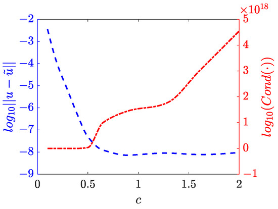
Figure 1. Variation of accuracy and condition number of the stiffness matrix with shape parameter c when $N_s=31$.

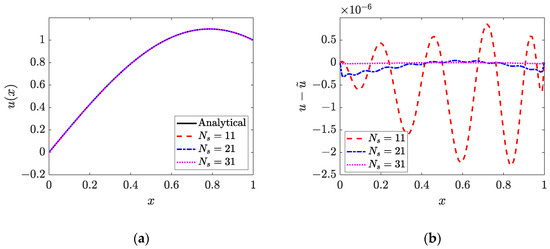
Figure 2. Solution and corresponding error for the 1D constant parameter identification problem: (a) solution; (b) corresponding error.

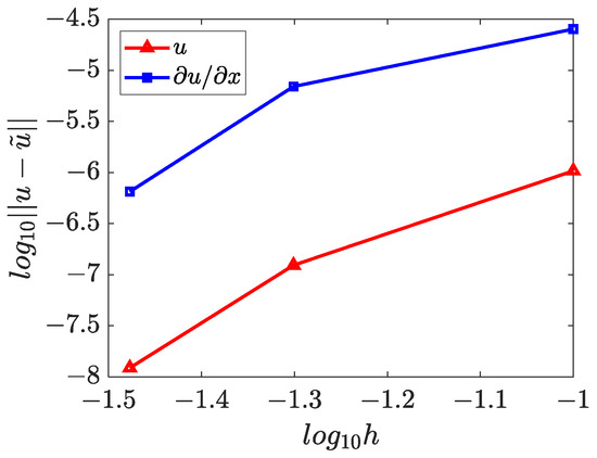
Figure 3. Convergence of the solutions for the 1D constant parameter identification problem.

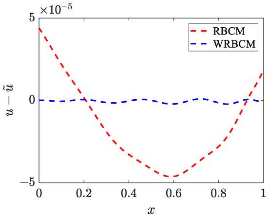
Figure 4. Solution comparison between RBCM and WRBCM for the 1D constant parameter identification problem.

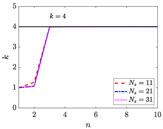
Figure 5. Variation of wave number $k$ with iteration steps for the 1D constant parameter identification problem.

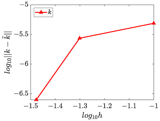
Figure 6. Convergence of wave number for the 1D constant parameter identification problem.

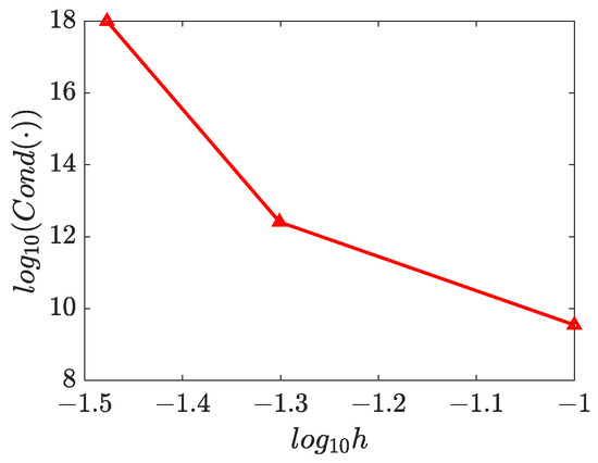
Figure 7. Condition number of stiffness matrix for the 1D constant parameter identification problem.

4.2. Two-Dimensional Inverse Helmholtz Problem of Constant Parameter Identification in Irregular Geometry

In this example, we study a two-dimensional (2D) inverse Helmholtz problem in irregular domain, as shown in Figure 8.

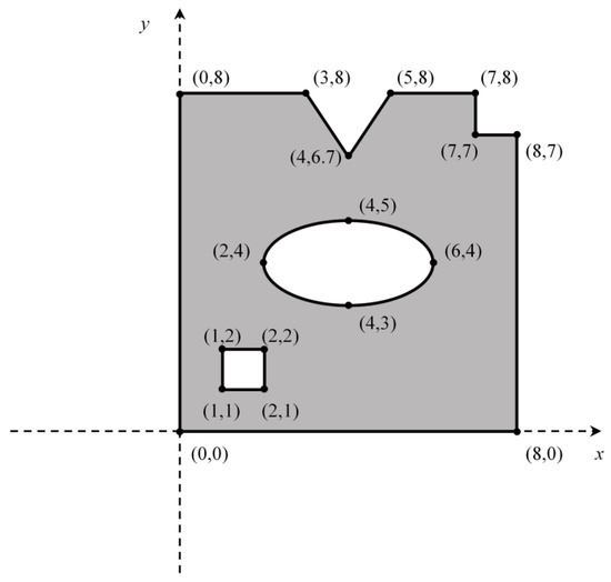
Figure 8. Configuration of 2D irregular geometry [33].

The governing equation and boundary conditions are given as follows

$$\frac{{\partial }^{2}u}{\partial x^2}+\frac{{\partial }^{2}u}{\partial y^2}+k^{2}u=0,\mathrm{in}\mathsf{\Omega }$$

(54)

$$\frac{\partial u}{\partial x}=\cos (x)\sin (y),\mathrm{on}x=0,y\in \left[0,8\right]$$

(55)

$$\frac{\partial u}{\partial y}=\sin (x)\cos (y),\mathrm{on}y=0,x\in \left[0,8\right]$$

(56)

$$u(x,y)=\sin (x)\sin (y),\mathrm{on}{\mathsf{\Gamma }}_g$$

(57)

where ${\mathsf{\Gamma }}_g={\displaystyle \underset{i=1}{\overset{11}{\cup }}{\mathsf{\Gamma }}_g{}^i}$ and

$$\begin{array}{l}{\mathsf{\Gamma }}_g{}^1=\left\{x=8,y\in \left[0,7\right]\right\},{\mathsf{\Gamma }}_g{}^2=\left\{y=8,x\in \left[0,3\right]\cup \left[5,7\right]\right\},{\mathsf{\Gamma }}_g{}^3=\left\{x=7,y\in \left[7,8\right]\right\},\\ {\mathsf{\Gamma }}_g{}^4=\left\{y=7,x\in \left[7,8\right]\right\},{\mathsf{\Gamma }}_g{}^5=\left\{1.3x+y-11.9=0,x\in \left[3,4\right],y\in \left[6.7,8\right]\right\},\\ {\mathsf{\Gamma }}_g{}^6=\left\{1.3x-y+1.5=0,x\in \left[4,5\right],y\in \left[6.7,8\right]\right\},{\mathsf{\Gamma }}_g{}^7=\left\{\frac{{(x-4)}^2}{4}+{(y-4)}^2=1,x\in \left[2,6\right],y\in \left[3,5\right]\right\}\\ {\mathsf{\Gamma }}_g{}^8=\left\{x=1,y\in \left[1,2\right]\right\},{\mathsf{\Gamma }}_g{}^9=\left\{x=2,y\in \left[1,2\right]\right\},{\mathsf{\Gamma }}_g{}^{10}=\left\{y=1,x\in \left[1,2\right]\right\},{\mathsf{\Gamma }}_g{}^{11}=\left\{y=2,x\in \left[1,2\right]\right\}\end{array}$$

(58)

An additional known condition is presented as

$$u(x,4)=\sin (x)\sin (4),\mathrm{on}\Pi$$

(59)

where $\Pi =\left\{y=4,x\in \left[0,2\right]\cup \left[6,8\right]\right\}$. The analytical solution is $u(x,y)=\sin (x)\sin (y)$ and the wave number that needs to be determined is $k=\sqrt{2}$. The error bound is set to be ${10}^{-10}$ for the iteration solutions. The weights imposed on the Dirichlet and measurement boundary conditions for this example are $\sqrt{w_{}^g}\approx \sqrt{w_{}^a}\approx 100$, and for the Neumann boundary condition is $\sqrt{w_{}^h}\approx 1$. The value of the shape parameter c is chosen to be 4, 2.2, 2 for the three discretization schemes, respectively.

Figure 9 and Figure 10 display the solutions of $u$ as well as its corresponding errors and the boundary errors under the discretization of $N_s=11\times 11,21\times 21$ and $31\times 31$, respectively. The errors are decreasing with refinement, which demonstrate that the proposed method can converge well in this inverse problem of the irregular domain. This is also illustrated in Figure 11, where the solutions converge exponentially. Figure 12 shows the iteration process of the unknown wave number, which indicates that this method can converge for the identification very quickly. The convergence of the identified wave number is exhibited in Figure 13. The solutions show that the exponential convergence can also be obtained for the unknown wave number identification. Figure 14 presents the condition number under different discretizations, where the condition number increases with the decrease in the node distance.

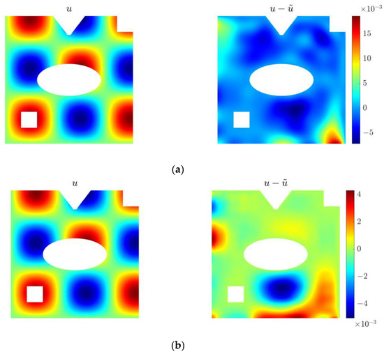
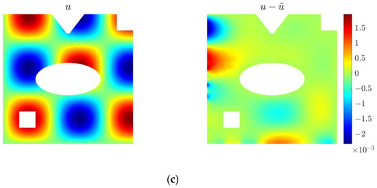
Figure 9. Solution and corresponding error for the 2D constant parameter identification problem in irregular geometry under different discretizations: (a) $N_s=11\times 11$; (b) $N_s=21\times 21$; (c) $N_s=31\times 31$.

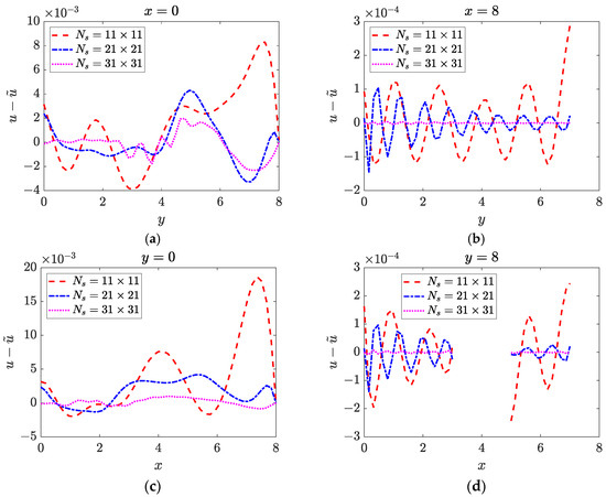
Figure 10. Boundary solutions for the 2D constant parameter identification problem in irregular geometry: (a) $x=0$; (b) $x=8$; (c) $y=0$; (d) $y=8$.

Figure 11. Convergence of the solutions for the 2D constant parameter identification problem in irregular geometry.

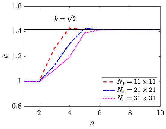
Figure 12. Variation of wave number $k$ with iteration steps for the 2D constant parameter identification problem in irregular geometry.

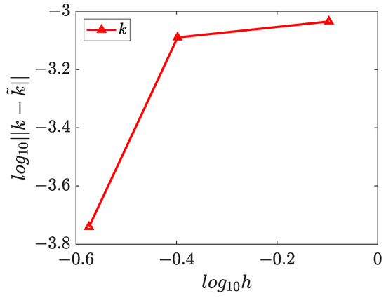
Figure 13. Convergence of wave number for the 2D constant parameter identification problem in irregular geometry.

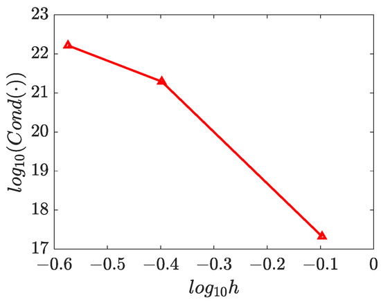
Figure 14. Condition number of stiffness matrix for the 2D constant parameter identification problem in irregular geometry.

4.3. Two-Dimensional Inverse Helmholtz Problem of Parameter Identification

After studying two examples of constant parameter identification, we further investigate a 2D inverse Helmholtz problem for identifying the varying parameter. The governing equation associated with boundary conditions can be expressed by

$$-\mathsf{\Delta }u\left(x,y\right)+k\left(x,y\right)u\left(x,y\right)=2\sin x\cos y+\frac{x^2\sin x\cos y}{2},\mathrm{in}\mathsf{\Omega },$$

(60)

$$u\left(x,y\right)=0,\mathrm{on}{\mathsf{\Gamma }}_g$$

(61)

The given known condition is

$$u\left(x,0\right)=\sin x,\mathrm{on}\Pi$$

(62)

The problem domain is $\mathsf{\Omega }=\left[0,\mathsf{\pi }\right]\times \left[-\frac{\mathsf{\pi }}{2},\frac{\mathsf{\pi }}{2}\right]$. ${\mathsf{\Gamma }}_g=\partial \mathsf{\Omega }$ denotes the Dirichlet boundary and $\Pi =\left\{y=0,x\in \left[0,\mathsf{\pi }\right]\right\}$ represents the subdomain for the measurement condition. The analytical solution for this problem is $u(x,y)=\sin x\cos y$, and the parameter that needs to be recognized is given as $k\left(x,y\right)=x^2/2$. The weights imposed on the boundary conditions are $\sqrt{w_{}^g}\approx \sqrt{w_{}^a}\approx 100$. The value of shape parameter c is chosen to be 3, 1.3, 0.85 for the three discretizations, respectively.

The numerical solutions for $u$ and $k$ are presented in Figure 15, Figure 16 and Figure 17, which demonstrate that the WRBCM can also achieve a high accuracy for solving the inverse Helmholtz problem of the varying parameter identification. The convergence studies for $u$ and $k$ are exhibited in Figure 18 and Figure 19, respectively. These indicate that for the varying parameter identification problem, the WRBCM can also acquire the exponential convergence for both the solutions and the identified parameter. The condition number of the stiffness matrix is shown in Figure 20, and a similar conclusion can be achieved, as in example 1 and 2.

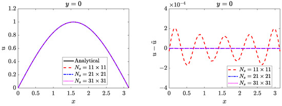
Figure 15. Solution and corresponding error for the 2D varying parameter identification problem.

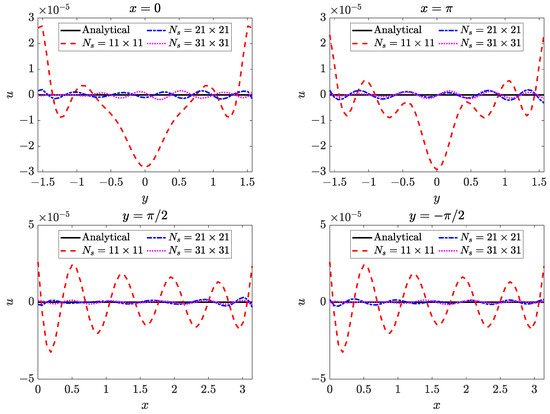
Figure 16. Boundary solutions for the 2D varying parameter identification problem.

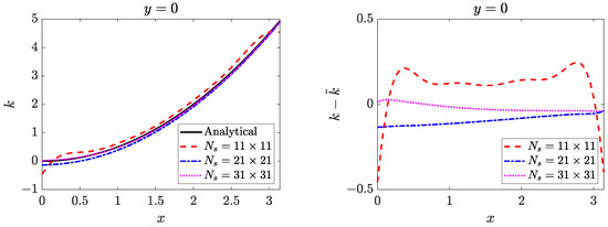
Figure 17. Solution and corresponding error of wave number $k$ for the 2D varying parameter identification problem.

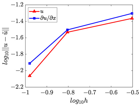
Figure 18. Convergence of the solutions for the 2D varying parameter identification problem.

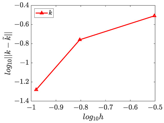
Figure 19. Convergence of wave number for the 2D varying parameter identification problem.

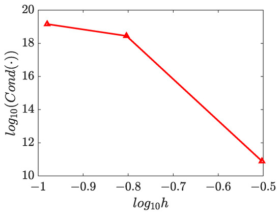
Figure 20. Condition number of stiffness matrix for the 2D varying parameter identification problem.

4.4. Three-Dimensional Inverse Helmholtz Problem of Parameter Identification in Cubic Domain

Next, a three-dimensional (3D) inverse Helmholtz problem of varying parameter identification in cubic domain is studied. The governing equation is described by

$$\frac{{\partial }^{2}u}{\partial x^2}+\frac{{\partial }^{2}u}{\partial y^2}+\frac{{\partial }^{2}u}{\partial z^2}+k(x,y,z)u=\left(x^2+y/2+z\right)\left(\sin x+\sin y+\sin z\right),\mathrm{in}\mathsf{\Omega }$$

(63)

$$u(x,y,z)=\sin (x)+\sin (y)+\sin (z),\mathrm{on}{\mathsf{\Gamma }}_g$$

(64)

The measurement condition on a plane is expressed as

$$u(0.5,y,z)=\sin (0.5)+\sin (y)+\sin (z),\mathrm{in}\Pi$$

(65)

where $\mathsf{\Omega }=\left[0,1\right]\times \left[0,1\right]\times \left[0,1\right]$, ${\mathsf{\Gamma }}_g=\partial \mathsf{\Omega }$ and $\Pi =\left\{x=0.5,y\in \left[0,1\right],z\in \left[0,1\right]\right\}$. The analytical solution and the identified parameter are given by

$$\begin{array}{c}u(x,y,z)=\sin (x)+\sin (y)+\sin (z)\\ k(x,y,z)=x^2+\frac{1}{2}y+z+1\end{array}$$

(66)

The weights for the boundary conditions are selected as $\sqrt{w_{}^g}\approx \sqrt{w_{}^a}\approx 100$, and the shape parameter is 3.3, 2.5, 1.7 for the three different discretizations, respectively.

Since the shape functions of RBFs are only depending on the radial distance from the origin, it is quite easy and straightforward to extend 1D problems to 2D and 3D problems. Once again, high accuracy can be obtained for solving the problem unknowns $u$ and $k$, as shown in Figure 21 and Figure 22, and exponential convergence can also be obtained for this 3D problem in cubic domain, as presented in Figure 23, Figure 24 and Figure 25 indicates that the WRBCM possesses high accuracy on the boundaries when proper weights are imposed on the boundary conditions during the solutions. Figure 26 presents the condition number of stiffness matrix for the 3D inverse problem. Once again, the refinement of the discretization increases the condition number, which has a negative effect on the stability.

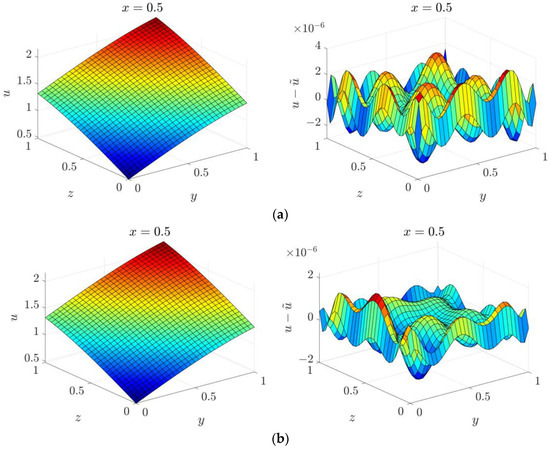
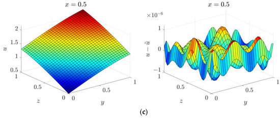
Figure 21. Solution and corresponding error for the 3D parameter identification problem in cubic domain under different discretizations: (a) $N_s=7\times 7\times 7$; (b) $N_s=9\times 9\times 9$; (c) $N_s=11\times 11\times 11$.

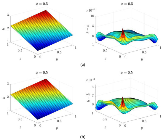
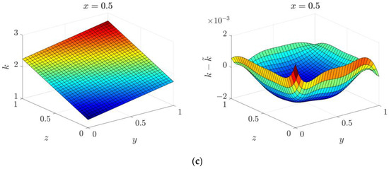
Figure 22. Solution of wave number $k$ for the 3D parameter identification problem in cubic domain under different discretizations: (a) $N_s=7\times 7\times 7$; (b) $N_s=9\times 9\times 9$; (c) $N_s=11\times 11\times 11$.

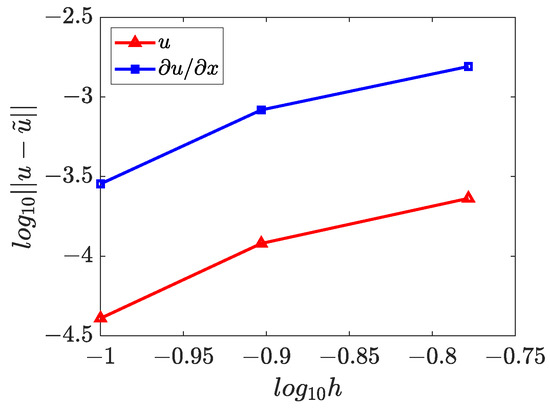
Figure 23. Convergence of the solutions for the 3D parameter identification problem in cubic domain.

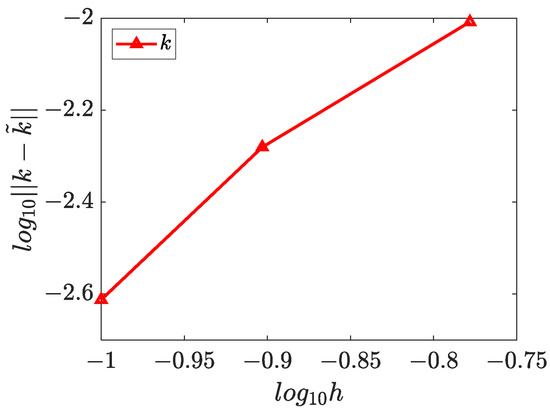
Figure 24. Convergence of wave number for the 3D parameter identification problem in cubic domain.

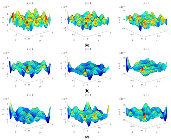
Figure 25. Errors of boundary solutions for the 3D parameter identification problem in cubic domain under different discretizations: (a) $N_s=7\times 7\times 7$; (b) $N_s=9\times 9\times 9$; (c) $N_s=11\times 11\times 11$.

Figure 26. Condition number of stiffness matrix for the 3D parameter identification problem in cubic domain.

4.5. Three-Dimensional Inverse Helmholtz Problem of Parameter Identification in Spherical Domain

We further consider another three-dimensional inverse Helmholtz problem of the parameter identification in spherical domain. The governing equation and boundary conditions are given as

$$\frac{{\partial }^{2}u}{\partial x^2}+\frac{{\partial }^{2}u}{\partial y^2}+\frac{{\partial }^{2}u}{\partial z^2}+k(x,y,z)u=\left(\frac{1}{2}x+y^2-z\right)\sin (x)\cos (y)\cos (z),\mathrm{in}\mathsf{\Omega }$$

(67)

$$u(x,y,z)=\sin (x)\cos (y)\cos (z),\mathrm{on}{\mathsf{\Gamma }}_g$$

(68)

where $\mathsf{\Omega }=\left\{x^2+y^2+z^2<1,x\in \left(-1,1\right),y\in \left(-1,1\right),z\in \left(-1,1\right)\right\}$, and ${\mathsf{\Gamma }}_g=\left\{x^2+y^2+z^2=1,x\in \left[-1,1\right],y\in \left[-1,1\right],z\in \left[-1,1\right]\right\}$. The measurement condition is given, as follows

$$u(x,0,z)=\sin (x)\cos (z),\mathrm{on}\Pi$$

(69)

The analytical solution is expressed by

$$u(x,y,z)=\sin (x)\cos (y)\cos (z)$$

(70)

and the wave number that needs to be identified is

$$k(x,y,z)=\frac{1}{2}x+y^2-z+3$$

(71)

Further, the weights imposed on the boundary conditions are provided as $\sqrt{w_{}^g}\approx \sqrt{w_{}^a}\approx 100$. The shape parameter is 2.5, 2 and 1.5, respectively.

The numerical solutions and boundary solutions of $u$ are displayed in Figure 27 and Figure 28, and the solutions of $k$ are presented in Figure 29. The results state that the WRBCM can obtain a high accuracy not only for the solution of the problem unknown $u$ but also for the solution of the identified parameter $k$. Moreover, high accuracy can also be achieved on the boundaries by imposing the appropriate weights. The convergence studies of $u$ and $k$ are shown in Figure 30 and Figure 31, which indicate that both solutions of $u$ and $k$ can receive exponential convergence. These results demonstrate that the WRBCM is a very good candidate for solving the nonlinear inverse Helmholtz problem of parameter identifications. Figure 32 displays the condition number for the 3D inverse problem in a spherical domain, and the condition number also follows the rules presented in the former examples

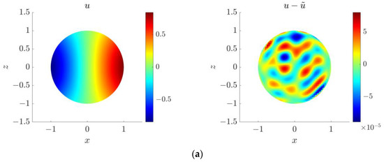
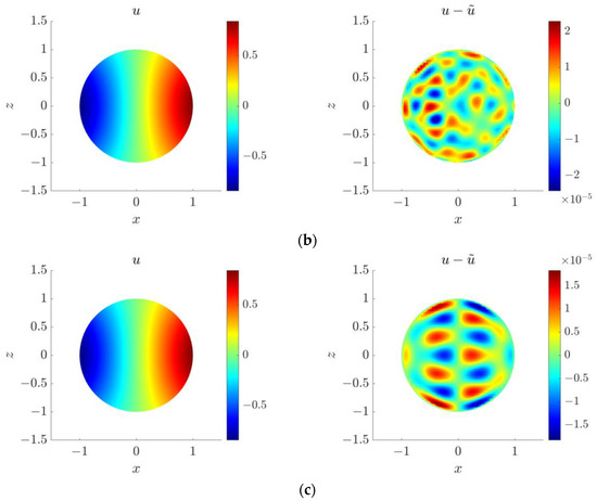
Figure 27. Solution and corresponding error at $y=0$ for the 3D parameter identification problem in spherical domain under different discretizations: (a) $N_s=7\times 7\times 7$; (b) $N_s=9\times 9\times 9$; (c) $N_s=11\times 11\times 11$.

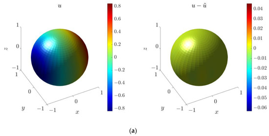
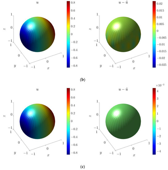
Figure 28. Boundary solution for the 3D parameter identification problem in spherical domain under different discretizations: (a) $N_s=7\times 7\times 7$; (b) $N_s=9\times 9\times 9$; (c) $N_s=11\times 11\times 11$.

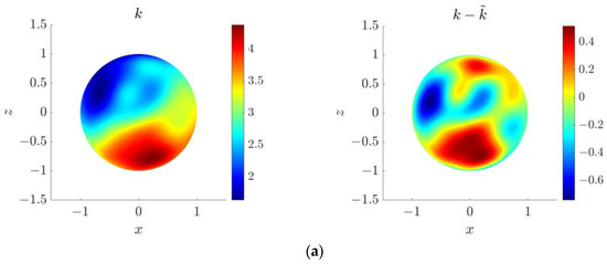
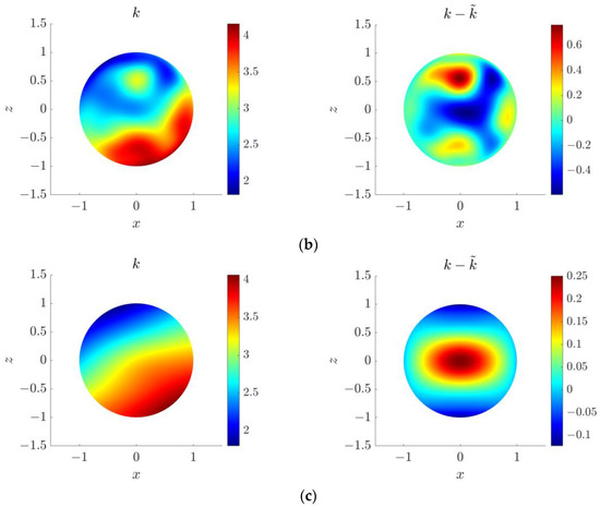
Figure 29. Solution and corresponding error of wave number $k$ for the 3D parameter identification problem in spherical domain under different discretizations: (a) $N_s=7\times 7\times 7$; (b) $N_s=9\times 9\times 9$; (c) $N_s=11\times 11\times 11$.

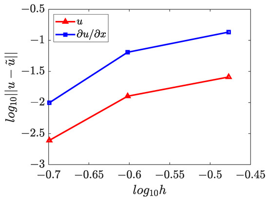
Figure 30. Convergence of the solutions for the 3D parameter identification problem in spherical domain.

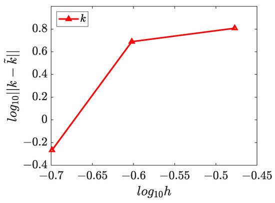
Figure 31. Convergence of wave number for the 3D parameter identification problem in spherical domain.

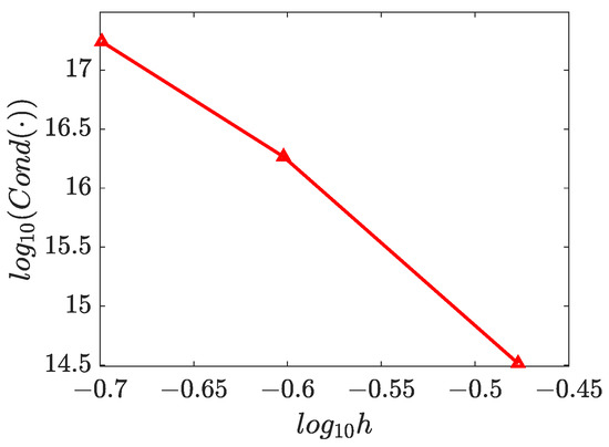
Figure 32. Condition number of stiffness matrix for the 3D parameter identification problem in spherical domain.

5. Conclusions

In this paper, a strong form weighted radial basis collocation method (WRBCM) combined with Newton’s iteration method is proposed to solve the nonlinear inverse Helmholtz problems of parameter identification. The radial basis collocation method (RBCM) using MQ-RBF possesses exponential convergence. Proper weights that should be imposed on the Neumann and Dirichlet boundary conditions as well as measurement conditions for achieving high accuracy and optimal convergence are mathematically derived. In the numerical examples, we investigate the influences of shape parameter on the accuracy and stability. Choosing an appropriate shape parameter can balance the solution accuracy and the condition number of the stiffness matrix, which affect the stability of the numerical solution. WRBCM is compared with the traditional RBCM in accuracy, and the solutions indicate that by adding proper weights on the boundary, the solution accuracy can be significantly improved. Numerical examples demonstrate that the proposed WRBCM can work well for 1D, 2D and 3D problems, and also has good performances on the inverse problem in both regular and irregular domains. We will extend this method for solving the inverse Helmholtz problems of other types, for example, boundary identification or source identification, etc., in the future work.

References

- Beskos, D.E. Boundary element methods in dynamic analysis: Part II (1986–1996). Appl. Mech. Rev. 1997, 50, 149–197. [Google Scholar] [CrossRef]
- Hall, W.S.; Mao, X.Q. A boundary element investigation of irregular frequencies in electromagnetic scattering. Eng. Anal. Bound. Elem. 1995, 16, 245–252. [Google Scholar] [CrossRef]
- Chen, J.T.; Wong, F.C. Dual formulation of multiple reciprocity method for the acoustic mode of a cavity with a thin partition. J. Sound Vib. 1998, 217, 75–95. [Google Scholar] [CrossRef]
- Wood, A.S.; Tupholme, G.E.; Bhatti, M.I.H.; Heggs, P.J. Steady-state heat transfer through extended plane surfaces. Int. Commun. Heat Mass Transf. 1995, 22, 99–109. [Google Scholar] [CrossRef]
- Shojaei, A.; Galvanetto, U.; Rabczuk, T.; Jenabi, A.; Zaccariotto, M. A generalized finite difference method based on the Peridynamic differential operator for the solution of problems in bounded and unbounded domains. Comput. Methods Appl. Mech. Eng. 2019, 343, 100–126. [Google Scholar] [CrossRef]
- Zienkiewicz, O.C. Achievements and some unsolved problems of the finite element method. Int. J. Numer. Methods Eng. 2000, 47, 9–28. [Google Scholar] [CrossRef]
- Onishi, K.; Kobayashi, K.; Ohura, Y. Numerical solution of a boundary inverse problem for the Laplace equation. Theor. Appl. Mech. 1996, 45, 257–264. [Google Scholar]
- Belytschko, T.; Krongauz, Y.; Organ, D.; Fleming, M.; Krysl, P. Meshless methods: An overview and recent developments. Comput. Methods Appl. Mech. Eng. 1996, 139, 3–47. [Google Scholar] [CrossRef]
- Liu, W.K.; Chen, Y.; Jun, S.; Chen, J.S.; Belytschko, T.; Pan, C.; Uras, R.A.; Chang, C. Overview and applications of the reproducing kernel particle methods. Arch. Comput. Methods Eng. 1996, 3, 3–80. [Google Scholar] [CrossRef]
- Oñate, E.; Perazzo, F.; Miquel, J. A finite point method for elasticity problems. Comput. Struct. 2001, 79, 2151–2163. [Google Scholar] [CrossRef]
- Liu, G.R.; Gu, Y. A point interpolation method for two-dimensional solids. Int. J. Numer. Methods Eng. 2001, 50, 937–951. [Google Scholar] [CrossRef]
- Cheng, A.D.; Cabral, J.J.S.P. Direct solution of ill-posed boundary value problems by radial basis function collocation method. Int. J. Numer. Methods Eng. 2005, 64, 45–64. [Google Scholar] [CrossRef]
- Wang, L.; Qian, Z. A meshfree stabilized collocation method (SCM) based on reproducing kernel approximation. Comput. Methods Appl. Mech. Eng. 2020, 371, 113303. [Google Scholar] [CrossRef]
- Wang, L.; Hu, M.; Zhong, Z.; Yang, F. Stabilized Lagrange Interpolation Collocation Method: A meshfree method incorporating the advantages of finite element method. Comput. Methods Appl. Mech. Eng. 2023, 404, 115780. [Google Scholar] [CrossRef]
- Wang, L. Radial basis functions methods for boundary value problems: Performance comparison. Eng. Anal. Bound. Elem. 2017, 84, 191–205. [Google Scholar] [CrossRef]
- Wang, L.; Liu, Y.; Zhou, Y.; Yang, F. Static and dynamic analysis of thin functionally graded shell with in-plane material inhomogeneity. Int. J. Mech. Sci. 2021, 193, 106165. [Google Scholar] [CrossRef]
- Liu, Z.; Xu, Q. A Multiscale RBF Collocation Method for the Numerical Solution of Partial Differential Equations. Mathematics 2019, 7, 964. [Google Scholar] [CrossRef]
- Dehghan, M.; Shokri, A. A meshless method for numerical solution of the one-dimensional wave equation with an integral condition using radial basis functions. Numer. Algorithms 2009, 52, 461–477. [Google Scholar] [CrossRef]
- Wang, L.; Chu, F.; Zhong, Z. Study of radial basis collocation method for wave propagation. Eng. Anal. Bound. Elem. 2013, 37, 453–463. [Google Scholar] [CrossRef]
- Hu, H.Y.; Chen, J.S.; Hu, W. Weighted radial basis collocation method for boundary value problems. Int. J. Numer. Methods Eng. 2007, 69, 2736–2757. [Google Scholar] [CrossRef]
- Zhang, X.; Song, K.Z.; Lu, M.W.; Liu, X. Meshless methods based on collocation with radial basis functions. Comput. Mech. 2000, 26, 333–343. [Google Scholar] [CrossRef]
- Liu, X.; Liu, G.R.; Tai, K.; Lam, K. Radial point interpolation collocation method (RPICM) for partial differential equations. Comput. Math. Appl. 2005, 50, 1425–1442. [Google Scholar] [CrossRef]
- Chen, J.S.; Hillman, M.; Chi, S.W. Meshfree methods: Progress made after 20 years. J. Eng. Mech. 2017, 143, 04017001. [Google Scholar] [CrossRef]
- Wang, L.; Zhong, Z. Radial basis collocation method for nearly incompressible elasticity. J. Eng. Mech. 2013, 139, 439–451. [Google Scholar] [CrossRef]
- Zheng, H.; Zhang, C.; Wang, Y.; Chen, W.; Sladek, J.; Sladek, V. A local RBF collocation method for band structure computations of 2D solid/fluid and fluid/solid phononic crystals. Int. J. Numer. Methods Eng. 2017, 110, 467–500. [Google Scholar] [CrossRef]
- Ferreira, A.J.M.; Roque, C.M.C.; Jorge, R.M.N. Free vibration analysis of symmetric laminated composite plates by FSDT and radial basis functions. Comput. Methods Appl. Mech. Eng. 2005, 194, 4265–4278. [Google Scholar] [CrossRef]
- Ferreira, A.J.M.; Fasshauer, G.E. Computation of natural frequencies of shear deformable beams and plates by an RBF-pseudospectral method. Comput. Methods Appl. Mech. Eng. 2006, 196, 134–146. [Google Scholar] [CrossRef]
- Chu, F.; Wang, L.; Zhong, Z.; He, J. Hermite radial basis collocation method for vibration of functionally graded plates with in-plane material inhomogeneity. Comput. Struct. 2014, 142, 79–89. [Google Scholar] [CrossRef]
- Ferreira, A.J.M.; Carrera, E.; Cinefra, M.; Roque, C.M.C.; Polit, O. Analysis of laminated shells by a sinusoidal shear deformation theory and radial basis functions collocation, accounting for through-the-thickness deformations. Compos. Part B Eng. 2011, 42, 1276–1284. [Google Scholar] [CrossRef]
- Chen, J.S.; Wang, L.; Hu, H.Y.; Chi, S.W. Subdomain radial basis collocation method for heterogeneous media. Int. J. Numer. Methods Eng. 2009, 80, 163–190. [Google Scholar] [CrossRef]
- Zerroukat, M.; Power, H.; Chen, C. A numerical method for heat transfer problems using collocation and radial basis functions. Int. J. Numer. Methods Eng. 1998, 42, 1263–1278. [Google Scholar] [CrossRef]
- Wang, L.; Chen, J.S.; Hu, H.Y. Subdomain radial basis collocation method for fracture mechanics. Int. J. Numer. Methods Eng. 2010, 83, 851–876. [Google Scholar] [CrossRef]
- Hon, Y.C.; Chen, W. Boundary knot method for 2D and 3D Helmholtz and convection–diffusion problems under complicated geometry. Int. J. Numer. Methods Eng. 2003, 56, 1931–1948. [Google Scholar] [CrossRef]
- Marin, L.; Lesnic, D. The method of fundamental solutions for the Cauchy problem associated with two-dimensional Helmholtz-type equations. Comput. Struct. 2005, 83, 267–278. [Google Scholar] [CrossRef]
- Marin, L. A meshless method for the numerical solution of the Cauchy problem associated with three-dimensional Helmholtz-type equations. Appl. Math. Comput. 2005, 165, 355–374. [Google Scholar] [CrossRef]
- Jin, B.; Zheng, Y. A meshless method for some inverse problems associated with the Helmholtz equation. Comput. Methods Appl. Mech. Eng. 2006, 195, 2270–2288. [Google Scholar] [CrossRef]
- Hon, Y.C.; Wei, T. A fundamental solution method for inverse heat conduction problem. Eng. Anal. Bound. Elem. 2004, 28, 489–495. [Google Scholar] [CrossRef]
- Shojaei, A.; Boroomand, B.; Soleimanifar, E. A meshless method for unbounded acoustic problems. J. Acoust. Soc. Am. 2016, 139, 2613–2623. [Google Scholar] [CrossRef]
- Shojaei, A.; Hermann, A.; Seleson, P.; Cyron, C.J. Dirichlet absorbing boundary conditions for classical and peridynamic diffusion-type models. Comput. Mech. 2020, 66, 773–793. [Google Scholar] [CrossRef]
- Hermann, A.; Shojaei, A.; Steglich, D.; Höche, D.; Zeller-Plumhoff, B.; Cyron, C.J. Combining peridynamic and finite element simulations to capture the corrosion of degradable bone implants and to predict their residual strength. Int. J. Mech. Sci. 2022, 220, 107143. [Google Scholar] [CrossRef]
- Li, M.; Jiang, T.; Hon, Y.C. A meshless method based on RBFs method for nonhomogeneous backward heat conduction problem. Eng. Anal. Bound. Elem. 2010, 34, 785–792. [Google Scholar] [CrossRef]
- Yu, Y.; Luo, X.; Zhang, H.; Zhang, Q. The Solution of Backward Heat Conduction Problem with Piecewise Linear Heat Transfer Coefficient. Mathematics 2019, 7, 388. [Google Scholar] [CrossRef]
- Wang, L.; Wang, Z.; Qian, Z. A meshfree method for inverse wave propagation using collocation and radial basis functions. Comput. Methods Appl. Mech. Eng. 2017, 322, 311–350. [Google Scholar] [CrossRef]
- Wang, L.; Wang, Z.; Qian, Z.; Gao, Y.; Zhou, Y. Direct collocation method for identifying the initial conditions in the inverse wave problem using radial basis functions. Inverse Probl. Sci. Eng. 2018, 26, 1695–1727. [Google Scholar] [CrossRef]
- Wang, L.; Qian, Z.; Wang, Z.; Gao, Y.; Peng, Y. An efficient radial basis collocation method for the boundary condition identification of the inverse wave problem. Int. J. Appl. Mech. 2018, 10, 1850010. [Google Scholar] [CrossRef]
- Hardy, R.L. Multiquadric equations of topography and other irregular surfaces. J. Geophys. Res. 1971, 76, 1905–1915. [Google Scholar] [CrossRef]
- Hardy, R.L. Research results in the application of multiquadratic equations to surveying and mapping problems. Surv. Mapp. 1975, 35, 321–332. [Google Scholar]
- Krige, D.G. A statistical approach to some basic mine valuation problems on the Witwatersrand. J. South. Afr. Inst. Min. Metall. 1951, 52, 119–139. [Google Scholar]
- Madych, W.R.; Nelson, S.A. Multivariate interpolation and conditionally positive definite functions. II. Math. Comput. 1990, 54, 211–230. [Google Scholar] [CrossRef]
- Li, Z.C.; Lu, T.T.; Hu, H.Y.; Cheng, A.H. Trefftz and Collocation Methods; WIT Press: Boston, MA, USA, 2008. [Google Scholar]
Disclaimer/Publisher’s Note: The statements, opinions and data contained in all publications are solely those of the individual author(s) and contributor(s) and not of MDPI and/or the editor(s). MDPI and/or the editor(s) disclaim responsibility for any injury to people or property resulting from any ideas, methods, instructions or products referred to in the content. |
© 2023 by the authors. Licensee MDPI, Basel, Switzerland. This article is an open access article distributed under the terms and conditions of the Creative Commons Attribution (CC BY) license (https://creativecommons.org/licenses/by/4.0/).