Abstract
Simple Summary
Discovering new drugs and innovating medical technology which targets the nervous system can be a challenge due to its complex nature. Over time, equations have been developed to model the behavior of neurons, the most basic units of the nervous system. Among these equations is the leaky integrate and fire model. Therefore, this research aims to compare two methods for estimating this model’s solution, which depicts the neurons’ behavior. The findings showed that Heun’s method estimated the model’s solution faster with higher accuracy and hence is more suitable for the leaky integrate and fire model.
Abstract
The human nervous system is one of the most complex systems of the human body. Understanding its behavior is crucial in drug discovery and developing medical devices. One approach to understanding such a system is to model its most basic unit, neurons. The leaky integrate and fire (LIF) method models the neurons’ response to a stimulus. Given the fact that the model’s equation is a linear ordinary differential equation, the purpose of this research is to compare which numerical analysis method gives the best results for the simplified version of this model. Adams predictor and corrector (AB4-AM4) and Heun’s methods were then used to solve the equation. In addition, this study further researches the effects of different current input models on the LIF’s voltage output. In terms of the computational time, Heun’s method was 0.01191 s on average which is much less than that of the AB-AM4 method (0.057138) for a constant DC input. As for the root mean square error, the AB-AM4 method had a much lower value (0.0061) compared to that of Heun’s method (0.3272) for the same constant input. Therefore, our results show that Heun’s method is best suited for the simplified LIF model since it had the lowest computation time of 36 ms, was stable over a larger range, and had an accuracy of 72% for the varying sinusoidal current input model.
Keywords:
computational neuroscience; numerical analysis; neuroinformatics; leaky integrate and fire (LIF); Adams predictor and corrector; Heun’s method MSC:
37N25
1. Introduction
From a biological perspective, the dendrites, soma, and axon are the three functionally distinct parts of a typical spiking neuron. The dendrites are the receiving ends of the neuron, which function as signal-collecting terminals (i.e., input terminals). The signals are then passed to the soma, which acts as the central processing unit that implements a nonlinear signal-refining process. As the signal propagates through the soma, an output is generated when the input exceeds a certain threshold. The output signal is then “fired off” or transmitted to the receiving neurons through the axon-terminal, manifested as short electrical pulses. These electrical pulses are also known as output spikes or action potentials, with voltages of about 100 mV that persist for 1 to 2 ms [,]. Synapses are defined as the interconnecting junctions between neurons, where signals are passed from one neuron’s end terminal to another neuron’s receiving terminal. Figure S1a shows an oversimplified illustration of the anatomy of the neuron [], including the dendrites, soma, and axon, while Figure S1b visualizes the depicted block diagram of a neuron [].
Neurotransmitters are chemical messenger molecules that transmit signals between different neurons or between neurons and other recipient cells (e.g., muscle cells). The process of neuron signaling is based on the generation of synapses which are fundamental in constructing more complex neural networks. There are two types of synapses: electrical and chemical []. Chemical synapses (Figure S2) occur when a presynaptic action potential propagates through the sending neuron and stimulates the release of neurotransmitters, which are stored at the presynaptic terminal in synaptic vesicles. While resting, neurons have a negative membrane potential []. When a nerve impulse reaches the axon’s terminal, depolarization effects cause the voltage-gated calcium ion channels to open and allow an influx of Ca2+ ions into the presynaptic terminal. The increased concentration of calcium ions induces the fusion of the loaded-synaptic vesicles with the membrane, thus the release of neurotransmitters []. These chemical messengers then diffuse through the synaptic cleft and bind to the postsynaptic receptors abundant on the signal-receiving side. The interaction between the neurotransmitter and the receptor is akin to the lock-and-key mechanism, as specific receptors bind specific signaling molecules. Thus, a physiological signal is generated in response to that certain neural activity. Generally, neurotransmitters can rapidly induce activation of ion channels and spawn fast synaptic transmission (e.g., acetylcholine (Ach) and epinephrine), or can modulate longer-lived actions that act on a protracted time scale (e.g., dopamine) [,]. Upon delivering the message, these neurotransmitters are terminated/inactivated to avoid excess buildup or diffusion to inappropriate synapses by (i) drifting and diffusing away from the synaptic cleft, (ii) moving away by transporter molecules, (iii) being reabsorbed by the sending neuron in a process known as reuptake, or (iv) being degrading by enzymes [].
While there are more than 100 well-identified neurotransmitters, they can be classified according to their chemical group []. Some of the common classes are (i) monoamines and acetylcholine, such as dopamine, serotonin, and histamine, (ii) amino acids, such as glutamate and glycine, (iii) purines, such as adenosine, (iv) lipids, such as anandamide, and (v) peptides such as oxytocin, somatostatin, and orexin []. Neurotransmitters can also be broadly categorized into excitatory, inhibitory, and modulatory based on the action they trigger at the postsynaptic end []. An excitatory neurotransmitter causes a neuron to “fire off” a signal that propagates to the next receiving neuron. For example, acetylcholine is an excitatory neurotransmitter that effectuates motivation, attention, and memory. On the contrary, an inhibitory neurotransmitter halts firing off an action potential; thus, the neural activity is terminated, and relaxation-like effects are induced []. Serotonin is an inhibitory neurotransmitter that plays a key role in mood regulation, sleep patterns, and sexual desire. Serotonin deficiency has been associated with anxiety, depression, appetite, and schizophrenia. Modulatory neurotransmitters, also known as neuromodulators, are unique in that they can simultaneously act on a larger number of target neurons [].
Table 1 lists some of the most common neurotransmitters associated with key functions in the human body. It is noteworthy to mention that some neurotransmitters, such as dopamine, can induce excitatory or inhibitory effects depending on the receptors present at the postsynaptic end. To elaborate, dopamine can inhibit the secretion of prolactin and mediate natural rewards in the brain []. Likewise, acetylcholine can have inhibitory effects on the heart (i.e., control the heart rate) or excitatory effects on neuromuscular junctions. Glutamate is the primary excitatory neurotransmitter, while GABA is the major inhibitory neurotransmitter in the central nervous system. Adrenaline and noradrenaline are excitatory neurotransmitters that play key roles in the fight or flight mechanism, whereas serotonin is an inhibitory neurotransmitter that aids in modulating mood and appetite [].

Table 1.
List of common neurotransmitters and their functions [,,].
The challenge of clearly understanding the brain’s complexity has long been a neuroscience focus. Using simplified models, researchers can investigate the computational processes associated with single neuron activity to aid in understanding the brain’s complexity. Then, single-neuron models can be used in larger network models that attempt to explain network computation, in addition to the benefits of clarifying mechanisms for single-neuron behavior [].
To illustrate, the Hodgkin–Huxley model describes how neurons initiate action potentials and how these signals propagate from one neuron to another by mapping between multiple variables, such as the membrane potential at equilibrium and the intracellular calcium concentration. Although it provides an understanding of such neuron behavior, it is complex, making it challenging to find suitable/accurate parameters and computationally expensive []. The neuron model shares many similarities with the electrical circuit; hence, it can be modeled using essential electrical components. The flow of the ions mimics the current, and the capacitance can describe the difference in the potential.
Equation (1) and Figure 1 show the Hodgkin–Huxley Model where I(t) is the current acting on the cell membrane, V(t) is the membrane potential, Cm is the membrane capacitance, gL is the membrane conductance, and EL is the equilibrium potential, also known as the “leak”. Hence, a more simplified model is required to simulate such behavior.
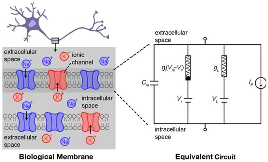
Figure 1.
Hodgkin–Huxley model describes the exchange of ionic species across the extracellular and intracellular space separated by a biological membrane. Cm refers to the membrane capacitance, t is time, Vm is the membrane voltage, VL is leakage voltage, and Ip is the ionic current through the ion pumps. Figure inspired from [].
The leaky integrate and fire (LIF) model is the linearized and simplified version of the Hodgkin–Huxley model. It is obtained from Equation (1) by replacing the INa + IK with a threshold for spike emission followed by a reset to a fixed potential. The expression IH + IAHP is omitted for simplification purposes. If included, the model is called the generalized leaky integrate and fire model (GLIF) [].
Therefore, the equation becomes:
where is the resting potential. After dividing by , Equation (3) is obtained:
Since the membrane resistance is inversely proportional to the conductance () and the time constant of the capacitor membrane is , the equation becomes:
The final ordinary differential equation (ODE) of the simplified LIF model is shown in Equation (5):
In addition, the following values of the parameters were found in the literature []: , , and such that at the beginning of time t = 0, the voltage is equal to the resting value (−75 mV). Substituting Equation (5) with these values will result in Equation (6):
Finally, the analytical or exact solution (7) of the LIF model with a current input with the initial condition of can be obtained by using the separation of variables with the necessary limits applied []:
Once a voltage threshold is crossed, the LIF model often inserts a spike, followed by decay, a step decrease, and/or a refractory period [].
Many works have compared the different spiking conditions and computed the computational cost of numerical methods (forward Euler, RK4, and exponential Euler) on the LIF with regular spiking, Hodgkin–Huxley, and Izhikevich [].
From a perspective of comparing the application of numerical analyses on different neuron models, AbdelAty et al. studied the fractional-order LIF (FO-LIF) and fractional-order Hodgkin–Huxley (FO-HH) model by applying numerical approximation methods, including the L1 algorithm, the Grunwald–Letnikov (GL) method, the FO-PI rectangular rule, and the Z-Transform approach []. It was found that the direction of adaptation varies between numerical approaches; for instance, the L1 approximation exhibits an upward spike frequency adaptation, while the PI-Rect rule exhibits a downward adaptation []. In another comparative study, Prada et al. used forward Euler to estimate the Neuroid and LIF models []. The Neuroid model is useful in understanding how functionally different neuron populations contribute to sensory information processing, but it has not been compared previously with other models in terms of computational cost and accuracy []. Their results showed that the Neuroid model is useful for a handful of applications. When computational resources are limited, Chicco et al. in [] concluded that the exponential Euler method is more suitable for the Hodgkin–Huxley model, RK4 for the Izhikevich modal, and forward Euler for the LIF model. Another example of examining multiple models was that of Syahid and Yuniati. They applied the Euler method and Hodgkin–Huxley, Izhikevich, and Wilson models to simulate the different spiking behaviors []. Their results show that both the LIF and Hodgkin–Huxley models can produce only regular spikes, unlike the other models that produce fast-spiking and intrinsic bursting.
Spiking patterns with LIF have been used in the past in conjunction with neural networks []. The authors choose to solve the model by explicit Euler. However, not an intuitive choice, second-order numerical approximation methods such as shooting methods have also been applied to find the LIF model’s most likely voltage path [].
Vidybida developed an interesting technique in [] to use their approximation algorithm to solve the LIF model by replacing floating point numbers with integer values which provided a more faithful representation of the binding neuron states and since floating points cause inaccuracies preventing exact comparison of such quantities [].
To focus more on the numerical analysis perspective, while the Euler method was widely popular in determining the exact solution of other neuron models, it does not fall short with several limitations, and hence, Heun’s method was developed. To provide further details concerning the origin of Heun’s method, Heun’s approach is built upon that of Euler’s []. Euler’s technique uses the line tangent to the function at the beginning of the interval to estimate the slope of the function over the interval because a small step size will result in a minor inaccuracy. However, even with minute step sizes, the estimate tends to deviate from the real functional value after a significant number of steps because of the accumulation of errors. In cases where the solution curve is concave upwards, its tangent line will overestimate the subsequent point’s vertical coordinate. Furthermore, the opposite will be true in cases where it is concave downwards. The vertical coordinates of all the points along the tangent line of the left end point, including the right endpoint of the interval under discussion, are smaller than those of the points that fall on the solution curve. Slightly steepening the slope is the key to solving this issue. Heun’s method takes into account the interval’s two tangent lines, one of which overestimates the ideal vertical coordinates and the other of which underestimates it. The slope of the right endpoint tangent alone, estimated by Euler’s method, must be used to build a prediction line. The result is too steep to be utilized as an ideal prediction line and overestimates the ideal point if this slope is passed via the interval’s left endpoint []. Heun’s method has several applications contributing to modern applications of science. For instance, it has been applied in deep learning applications such as Maleki et al.’s newly developed “HeunNet”, a neural network model that improves the performance of ResNet []. It has also been applied to emerging health challenges similar to Fatoba’s study where it was used to solve the model of the susceptible, infectious, recovery, and death (SIRD) COVID-19 model []. However, its potential has not been discovered in solving LIF models.
Another model worth highlighting is the Adams predictor and corrector method (AB4-AM4). Yucedag and Dalkiran [] applied several numerical analysis techniques (including AB4-AM4) on the Hodgkin–Huxley, FitzHugh–Nagumo, Morris–Lecar, Hindmarsh–Rose, and Izhikevich neuron models. They compared simulation and experimentation results by implementing the models on a Raspberry Pi. This method yielded the least errors for the implementation of the Izhikevich on Raspberry Pi compared to the simulation results. However, their study was limited to the external digital-to-analog converter’s sampling rate, which could have partially contributed to this error. It was needed since the Raspberry Pi does not have existing analog outputs []. Similar implementation studies also compared similar models but with different hardware, such as a field programmable gate array []. In all cases, none of these studies explored AB4-AM4’s application on the LIF model, which further emphasizes the novelty of this study.
Although modeling neurons with the Hodgkin–Huxley model and others have many disadvantages/drawbacks, the LIF model requires 95% fewer computations than the other neuron models [], and their full capacity with different numerical approximations is a compelling branch of work. This research aims to study which numerical analysis method is best suited for solving the LIF ordinary equation by applying Heun and Adams predictor and corrector (AB4-AM4) methods and calculating their error values as the computation time. This research also studies the effect of different input current models on the output membrane potential voltage using the same LIF model.
2. Materials and Methods
Researchers have previously applied numerical analysis to the family of LIF models. For example, Sharma et al. [] compared the finite element method (FEM) and the weighted essentially non-oscillatory (WENO) finite difference approximation on a nonlinear noisy LIF model and found that the FEM approach might yield better results compared to WENO. In addition, a postgraduate summer computational neuroscience summer school [] applied the implicit Euler method to calculate the neurons’ membrane potential (V). On the other hand, no study has attempted to apply Heun’s method and other numerical approximation methods to the simplified LIF model. Therefore, we chose Heun’s method and AB4-AM4 for our analysis.
2.1. Heun’s Method
Heun’s method, also known as the improved Euler’s method, is a numerical technique for analyzing first-order ordinary differential equations []. Heun’s method is also considered the 2nd-order Runge Kutta (RK2) method and is more accurate than the original Euler methods by correcting the error of these methods through a mean slope [].
Equation (8) shows the mathematical expression of this method:
where dt is the step size, is the corrector, and is the predictor.
Stability is a concern in ordinary differential equations such that an equation is considered stable if its solution behaves in a controlled and bounded way. Concerning the stability of Heun’s method, according to [], it is conditionally stable based on Equations (9) and (10), given that (⊆) where S is the stability function:
Based on [], Equation (11) shows the time step values that ensure stability using Heun’s method.
Figure 2 shows the stability plot for Heun’s method. For our specific equation, since V is multiplied by in Equation (5). Therefore, the stability condition becomes as shown in Equation (11).
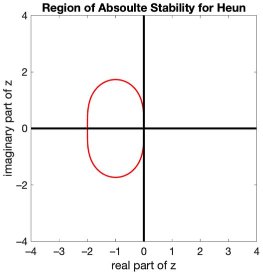
Figure 2.
Global absolute stability region for Heun’s method.
The region of absolute stability for Heun’s method, presented in Figure 2, is the region translated in the complex z plane. The figure depicts that the absolute region for Heun’s method is centered around −1 and has an interval of {−2,0}, as concluded from Equation (11). However, each ODE will depend on “ where is allowed to be complex as, in reality, it portrays the eigenvalue of the Jacobi matrix.
2.2. The AB4-AM4 Method
Adams methods belong to the family of multipoint methods. They were also developed over the finite grid rather than finite-element-based approaches but are coupled with Newton’s difference polynomial. They can be understood as the aggregation of the kth-degree Newton back difference polynomial. Like Euler’s methods, they can be classified as explicit and implicit, where the explicit is termed as the Adams–Bashforth (AB) method and the latter is termed as the Adams–Moulton (AM) method [].
The implicit AM does not suffer from numerical instability, whereas AB is unstable for relatively large values of differential time (dt). Since both AM and AB are fourth-order accurate, they are best used in conjunction as predictors and correctors. More specifically, AB is used as the predictor, whereas AM is used as a corrector.
The number of steps can be chosen to be two or four, which is dictated by k; in the two-step method, only the last step and the point itself are considered, whereas when using the four-step method, the consecutive three previous time stamps need to be considered.
Adams methods are widely used in targeting stiff equations. The capacitance modeled in the equation can exhibit stiff behavior and thus motivates using Adam. Another motivation for using AB4-AM4 is that it solves multiplicative initial value problems, which is the case of the LIF model []. They are also known to be less computationally extensive compared to Runge–Kutta methods [].
AB4-AM4 predictor and corrector formulas are given in Equations (12) and (13), respectively.
The stability analysis is crucial for all of the techniques as they provide the validity of the results in conjunction with the methods being applied.
A method qualifies to be stable if it produces bounded solutions for a stable ODE; the amplification factor or gain (G) that describes the relationship between the solution at the current time stamp with the preceding is employed []. Thus, the gain polynomial was used to draw reasonable conclusions regarding the stability.
The gain equation (14) for stability yielded for AB4-AM4 is dependent on the variables dt and α, the constant dictating our ODE. The α derived from the original ODE is 1/τ, where τ was 10.
And dt is again the step size.
The equation was solved by finding the roots of the equations for a set of dt values; the four gains were found, which were complex, and for concluding, the absolute polar component of each G must be strictly less than one, as indicated by the horizontal line in the figure.
Each G in the equation can be denoted as G1, G2, and so forth, depending on the power. Solving for dt where Gs are equal or less than one will dictate the value of dt for stable behavior. The last two Gs (G3 and G4) are equal by the nature of the equation. The results obtained are presented in Figure 3, and they illustrate the conditions for stability as well and dt required to maintain it. As seen from the graph, dt = 30 ms is the point that satisfies the condition of all |Gs|to be less than one. The maximum timestamp 30 ms was also indicated in the figure in a red dashed line.
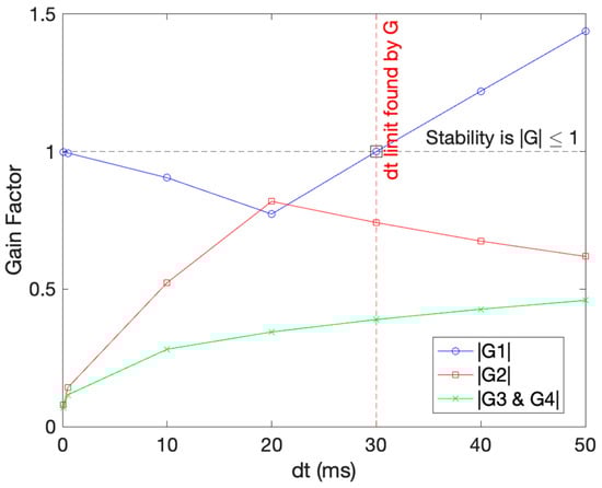
Figure 3.
Stability analysis for the AB4-AM4 method on our ODE. The black dotted line represents the G limit that must be abided by, and the red vertical line shows the dt found abiding by the limit.
3. Results and Discussion
3.1. Heun’s Method
Based on Heun’s stability condition for this specific LIF model, step size values were studied to see the instability effect. Figure 4 shows the effect of these values below and above 20 ms, specifically dt = 0.2 ms and dt = 50 ms. At a step size of 0.2 ms and lower, it was found that the numerical Heun’s solution had a similar behavior compared to the true and exact graph. However, at a step size of 5 ms and above, it was shown that the solution has an irregular behavior for a time interval of less than 100 ms, indicating an error-prone behavior. The unstable behavior is declared in Figure 2 and therefore, it can be concluded that Heun’s method is indeed conditionally stable, more precisely for step size values between 0 and 20 ms. Though it is not a precise judgment of stability, it is a rough approximation of the oscillation and finding the fallacy of solutions.
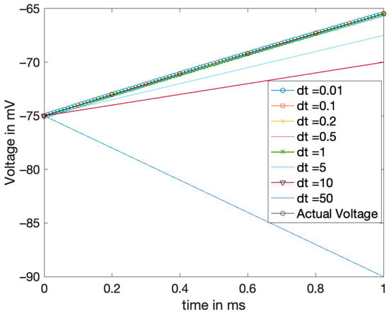
Figure 4.
Stability analysis for Heun’s method: Solutions with different step sizes ‘dt’ plotted and the behavior in matching true solutions observed.
The value that was tested beyond the stable region was 50 ms, and the solution completely diverges for that case.
From Figure 5, the membrane potential exponentially increases from −75 mV, then plateaus at 20 mV after a certain time, indicating that the neuron is excited, transmitting this signal to a neighboring neuron. While it is not the most accurate representation of the real behavior of a neuron (neurons are noisier and more complex), it does suffice for efficient modeling.
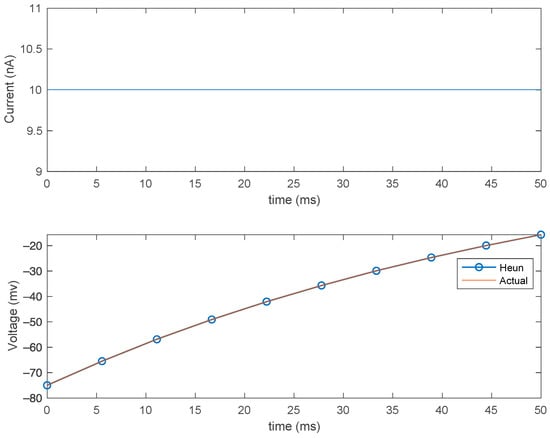
Figure 5.
Effect of the constant current on the membrane (top) and Heun’s method compared with analytical solution (bottom) for step size (dt) = 0.2 ms.
3.2. AB4-AM4 Method
The AB4-AM4 method was implemented on MATLAB, where the four initial guesses were sourced from RK4. Based on the stability analysis, the values for time stamps of interest were less than 30 ms.
However, swept analyses were performed, as shown in Figure 6b to affirm the unstable behavior of the solution obtained, passing the dt limit.
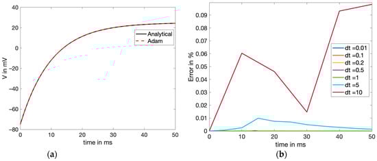
Figure 6.
(a) AB4-AM4 method comparison with the exact (analytical) solution, both plotted to approximate the voltage in the membrane with the DC input current, and (b) error comparison (exact-calculated) for different step size values of the AB4-AM4 numerical solution.
The results observed in Table 2 show that for the DC input, the accuracy was highest for dt = 0.01 ms, with the computational time being the most. Nonetheless, since the errors for all the values of dt were within reasonable limits for 0.01 < dt < 30, any dt from that range should suffice as a suitable choice. Though 30 ms is the maximum limit for stability, it can be observed that the error starts increasing beyond 5 ms. Usually, a good choice for the step size is at least 50% or less than the maximum size to prevent overshoot. Since dt = 0.2 ms seemed to give the best results and the trade-off between the computational cost and accuracy was minuscule, it was chosen for the comparative results and was plotted against the exact solution, as shown in Figure 6a. The values of dt below 1 are all very accurate and generate a minimal error; it is even hard to distinguish between them, as in Figure 6b, whereas the unstable error from dt = 10 is prevalent.
Table 2.
Heun’s method and AB4-AM4 comparative analysis for DC input.
3.3. Comparison of Numerical Methods
Table 1 summarizes the computation time, absolute mean percentage error, and absolute root means square error results of both Heun’s method and the AB4-AM4 method based on different dt values. To find the accuracy at each time step for each method, the absolute mean percentage error is applied, Equation (15):
Averaging Equation (15) will result in the absolute mean percentage error.
Another metric for assessing the accuracy is the root mean square error (RMSE) [], which is governed by Equation (16):
Based on Table 2 and the effect of the step size on the computation time and the two types of errors, the smaller the step size is, the fewer errors both of the numerical methods encounter, but the more computationally expensive it becomes to compute them with time.
Whist comparing Heun’s method and the AB4-AM4 method, Heun’s method is faster in computation time than AB4-AM4, but AB4-AM4 has fewer errors compared to Heun’s method. In that case, both methods have a trade-off between time and accuracy. In addition, the execution of these methods also depends on the available computational resources. For instance, a supercomputer might hypothetically be able to finalize computing both Heun’s method and the AB4-AM4 method in relatively the same amount of time. In such a case, one model could be more laborious and energy-intensive compared to the other. Therefore, it depends on the purpose of using the LIF model. If it is for rapid prototyping of medical devices for treating neuromuscular disorders, for instance, then Heun’s method would be a better choice for solving the model, as it provides reasonable accuracy in a shorter time.
On the other hand, if the application does not have a strict time constraint and there is a higher need for accuracy in understanding the behavioral mechanisms of a neuron, then the AB4-AM4 method would be the appropriate method.
3.4. Comparison of the Alternating Current (AC) Input Current with the Constant Current (DC)
In nature, the bioelectric current is not constant but rather varies with time. For simplification purposes in this work, our study modeled the bioelectric current as a constant. We also aim to study the effect of other commonly used input current models. Some researchers [] resorted to a simple sinusoidal current to simulate such signals’ varying with time. Equation (17) [] shows the alternating sinusoidal current model, also depicted in Figure 7, with a frequency of 6 MHz:
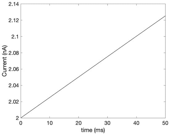
Figure 7.
The varying input current.
The simplified LIF model was numerically approximated with the AB4-AM4 method with varying input for the same range. The results showed that the numerical method could be approximated by varying the conditions of the model. Figure 8 shows the estimated output voltage with varying current conditions.
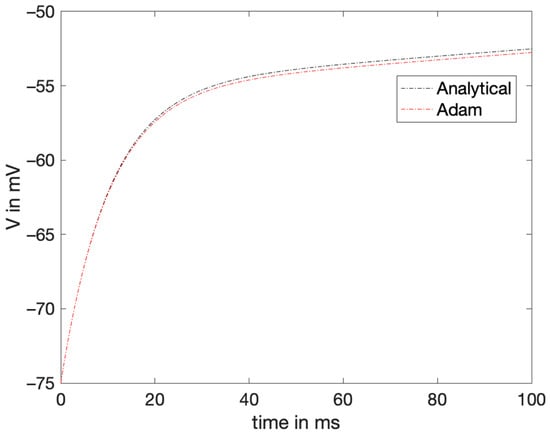
Figure 8.
The estimated voltage from the AM4-AB4 method versus the exact voltage plotted when the current is also varying.
The MAE and RMSE were obtained to be 0.2796 and 0.0582, respectively. Though these results are good approximations, they show that more variables must be added to the original LIF model to manage more complex inputs and move closer to modeling the actual neuron behavior.
Since these methods are based on the last or multiple last calculated values, the error aggregates and grows if the preceding value is not accurate. Therefore, it needs to be ensured that the error at each step is minimized, which gives room for adaptive techniques, which are a few techniques that can be explored in these methods.
In one of their studies, Shelley and Tao studied the effect of the time step of RK2 and RK4 on a LIF model with spikes []. They found that to achieve a six-digit accuracy, a time step of for RK4 and for RK2 was required. As for the choices on step sizes, a smaller step size results in fewer approximation errors for the LIF model for the numerical analysis [,,], as it would intuitively. The results obtained in this study are very close and provide a good approximation.
Whilst other researchers did apply numerical methods to LIF models with spikes and sometimes with noise, this study also studies the computational cost and time step of the AB4-AM4 method. It also compares its performance with Heun’s method in both constant and varying inputs of the current of the LIF model.
4. Conclusions
In conclusion, this paper discusses the importance of modeling neurons, specifically using the simplified LIF model, to understand their behavior better. Since the model is an ordinary differential equation, we proposed two numerical methods that have not been previously applied to this equation. It was found that Heun’s method (a second-order method) provides reasonable and precise estimates with good computational costs for our time-sensitive application. Since the tested models are still not extensively inclusive of real-life mimicking of neurons, the future perspective involves incorporating a spike behavior to the voltage for a more realistic model of the neurons’ behavior. Furthermore, simulating various additive white gaussian noises along with current input are to be explored as those aid in mimicking the most accurate behavior of a neuron.
Supplementary Materials
The following supporting information can be downloaded at: https://www.mdpi.com/article/10.3390/math11030714/s1, Figure S1: (a) Anatomy of a Single Neuron (b) Depicted Block Diagram of a Neuron; Figure S2: Summary of the process of synapsis generation and neuro-signaling.
Author Contributions
Conceptualization, G.E.M.; methodology, G.E.M., A.A., W.H.A. and M.M.; software, A.A. and G.E.M.; validation, G.E.M., A.A. and M.M.; formal analysis, G.E.M. and A.A.; writing—original draft preparation, G.E.M., A.A. and W.H.A.; writing—review and editing, G.E.M., A.A., W.H.A., M.M. and G.A.H.; supervision, M.M. and G.A.H. All authors have read and agreed to the published version of the manuscript.
Funding
We would like to acknowledge student funding from the Biomedical Engineering M.S. program at AUS. The authors would also like to acknowledge the financial support of the American University of Sharjah Faculty Research Grants, Al-Jalila Foundation (AJF 2015555), Al Qasimi Foundation, Patient’s Friends Committee of Sharjah, Biosciences and Bioengineering Research Institute (BBRI18-CEN-11), GCC Co-Fund Program (IRF17-003), the Takamul program (POC-00028-18), Technology Innovation Pioneer (TIP) Healthcare Awards, Sheikh Hamdan Award for Medical Sciences MRG/18/2020, Friends of Cancer Patients (FoCP), and Dana Gas Endowed Chair for Chemical Engineering. The work in this paper was supported, in part, by the Open Access Program of the American University of Sharjah (OAPCEN-1410-E00131). This paper represents the opinions of the author(s) and does not mean to represent the position or opinions of the American University of Sharjah.
Institutional Review Board Statement
Not applicable.
Informed Consent Statement
Not applicable.
Data Availability Statement
Not applicable.
Conflicts of Interest
The authors declare no conflict of interest.
References
- Van De Burgt, Y.; Gkoupidenis, P. Organic materials and devices for brain-inspired computing: From artificial implementation to biophysical realism. MRS Bull. 2020, 45, 631–640. [Google Scholar] [CrossRef]
- Salman, A.M.; Malony, A.D.; Sottile, M.J. An Open Domain-Extensible Environment for Simulation-Based Scientific Investigation (ODESSI). In Proceedings of the Computational Science–ICCS 2009, 9th International Conference, Baton Rouge, LA, USA, 25–27 May 2009; pp. 23–32. [Google Scholar] [CrossRef]
- Vazquez, R.A.; Cachón, A. Integrate and fire neurons and their application in pattern recognition. In Proceedings of the 2010 7th International Conference on Electrical Engineering Computing Science and Automatic Control, Tuxtla Gutierrez, Mexico, 8–10 September 2010; pp. 424–428. [Google Scholar]
- Teeter, C.; Iyer, R.; Menon, V.; Gouwens, N.; Feng, D.; Berg, J.; Szafer, A.; Cain, N.; Zeng, H.; Hawrylycz, M.; et al. Generalized leaky integrate-and-fire models classify multiple neuron types. Nat. Commun. 2018, 9, 709. [Google Scholar] [CrossRef] [PubMed]
- Schweizer, F.E. Neurotransmitter release from presynaptic terminals. eLS 2001. [CrossRef]
- Alberts, B.; Johnson, A.; Lewis, J.; Raff, M.; Roberts, K.; Walter, P. Ion channels and the electrical properties of membranes. In Molecular Biology of the Cell, 4th ed.; Garland Science: New York City, NY, USA, 2002. [Google Scholar]
- Fon, E.A.; Edwards, R.H. Molecular mechanisms of neurotransmitter release. Muscle Nerve Off. J. Am. Assoc. Electrodiagn. Med. 2001, 24, 581–601. [Google Scholar] [CrossRef]
- Hyman, S.E. Neurotransmitters. Curr. Biol. 2005, 15, R154–R158. [Google Scholar] [CrossRef]
- Sheffler, Z.M.; Reddy, V.; Pillarisetty, L.S. Physiology, Neurotransmitters; StatPearls Publishing: Treasure Island, FL, USA, 2022. [Google Scholar]
- Juárez Olguín, H.; Calderón Guzmán, D.; Hernández García, E.; Barragán Mejía, G. The role of dopamine and its dysfunction as a consequence of oxidative stress. Oxidative Med. Cell. Longev. 2016, 2016, 9730467. [Google Scholar] [CrossRef] [PubMed]
- Neuromatch Academy. Tutorial 1: The Leaky Integrate-and-Fire (LIF) Neuron Model. Available online: https://compneuro.neuromatch.io/tutorials/W2D3_BiologicalNeuronModels/student/W2D3_Tutorial1.html (accessed on 28 November 2022).
- Neuromatch Academy. Tutorial 3: Numerical Methods. Available online: https://compneuro.neuromatch.io/tutorials/W0D4_Calculus/student/W0D4_Tutorial3.html (accessed on 28 November 2022).
- Long, L.; Gupta, A. Biologically-Inspired Spiking Neural Networks with Hebbian Learning for Vision Processing. In Proceedings of the 46th AIAA Aerospace Sciences Meeting and Exhibit, Reno, NV, USA, 7–10 January 2008. [Google Scholar] [CrossRef]
- Chicco, D.; Warrens, M.J.; Jurman, G. The coefficient of determination R-squared is more informative than SMAPE, MAE, MAPE, MSE and RMSE in regression analysis evaluation. PeerJ Comput. Sci. 2021, 7, e623. [Google Scholar] [CrossRef]
- AbdelAty, A.; Fouda, M.; Eltawil, A. On numerical approximations of fractional-order spiking neuron models. Commun. Nonlinear Sci. Numer. Simul. 2021, 105, 106078. [Google Scholar] [CrossRef]
- Prada, E.J.A.; Arteaga, I.A.B.; Martínez, A.J.D. The Neuroid revisited: A heuristic approach to model neural spike trains. Res. Biomed. Eng. 2017, 33, 331–343. [Google Scholar] [CrossRef]
- Syahid, A.; Yuniati, A. Simulation of spiking activities neuron models using the Euler method. J. Phys. Conf. Ser. 2021, 1951, 012065. [Google Scholar] [CrossRef]
- Paninski, L. The most likely voltage path and large deviations approximations for integrate-and-fire neurons. J. Comput. Neurosci. 2006, 21, 71–87. [Google Scholar] [CrossRef] [PubMed]
- Vidybida, A. Simulating leaky integrate-and-fire neuron with integers. Math. Comput. Simul. 2018, 159, 154–160. [Google Scholar] [CrossRef]
- Iyasele, K.E. A Study of Some Computational Algorithms for Solving First Order Initial Value Problems. Bachelor’s Thesis, Federal University Oye-Ekiti, Oye-Ekiti, Nigeria, August 2015. [Google Scholar]
- Maleki, M.; Habiba, M.; Pearlmutter, B.A. HeunNet: Extending ResNet using Heun’s Method. In Proceedings of the 2021 32nd Irish Signals and Systems Conference (ISSC), Athlone, Ireland, 10–11 June 2021; pp. 1–6. [Google Scholar]
- Akogwu, B.O.; Fatoba, J. Numerical solutions of COVID-19 SIRD model in Nigeria. FUDMA J. Sci. 2022, 6, 60–67. [Google Scholar]
- Yucedag, V.B.; Dalkiran, I. A Raspberry Pi Based Hardware Implementations of Various Neuron Models; Research Square: Durham, NC, USA, 2022. [Google Scholar] [CrossRef]
- Tolba, M.; El-Safty, A.; Armanyos, M.; Said, L.A.; Madian, A.; Radwan, A.G. Synchronization and FPGA realization of fractional-order Izhikevich neuron model. Microelectron. J. 2019, 89, 56–69. [Google Scholar] [CrossRef]
- Sharma, D.; Singh, P.; Agarwal, R.P.; Koksal, M.E. Numerical Approximation for Nonlinear Noisy Leaky Integrate-and-Fire Neuronal Model. Mathematics 2019, 7, 363. [Google Scholar] [CrossRef]
- Workie, A.H. New Modification on Heun’s Method Based on Contraharmonic Mean for Solving Initial Value Problems with High Efficiency. J. Math. 2020, 2020, 6650855. [Google Scholar] [CrossRef]
- Amir Taher, K. Comparison of Numerical Methods for Solving a System of Ordinary Differential Equations: Accuracy, Stability and Efficiency. Bachelor’s Thesis, Mälardalens University, Västerås, Sweden, 2020. [Google Scholar]
- Ghrist, M.L.; Fornberg, B.; Reeger, J.A. Stability ordinates of Adams predictor-corrector methods. BIT Numer. Math. 2014, 55, 733–750. [Google Scholar] [CrossRef]
- Misirli, E.; Gurefe, Y. Multiplicative adams bashforth–moulton methods. Numer. Algorithms 2011, 57, 425–439. [Google Scholar] [CrossRef]
- Hoffman, J.D.; Frankel, S. Numerical Methods for Engineers and Scientists; CRC Press: Boca Raton, FL, USA, 2018. [Google Scholar]
- Shelley, M.J.; Tao, L. Efficient and accurate time-stepping schemes for integrate-and-fire neuronal networks. J. Comput. Neurosci. 2001, 11, 111–119. [Google Scholar] [CrossRef]
- Teka, W.; Marinov, T.M.; Santamaria, F. Neuronal Spike Timing Adaptation Described with a Fractional Leaky Integrate-and-Fire Model. PLoS Comput. Biol. 2014, 10, e1003526. [Google Scholar] [CrossRef]
- Hu, J.; Liu, J.-G.; Xie, Y.; Zhou, Z. A structure preserving numerical scheme for Fokker-Planck equations of neuron networks: Numerical analysis and exploration. J. Comput. Phys. 2021, 433, 110195. [Google Scholar] [CrossRef]
- Singh, P.; Kadalbajoo, M.K.; Sharma, K. Probability density function of leaky integrate-and-fire model with Lévy noise and its numerical approximation. Numer. Anal. Appl. 2016, 9, 66–73. [Google Scholar] [CrossRef]
- Valadez-Godínez, S.; Sossa, H.; Santiago-Montero, R. On the accuracy and computational cost of spiking neuron implementation. Neural Netw. 2019, 122, 196–217. [Google Scholar] [CrossRef] [PubMed]
Disclaimer/Publisher’s Note: The statements, opinions and data contained in all publications are solely those of the individual author(s) and contributor(s) and not of MDPI and/or the editor(s). MDPI and/or the editor(s) disclaim responsibility for any injury to people or property resulting from any ideas, methods, instructions or products referred to in the content. |
© 2023 by the authors. Licensee MDPI, Basel, Switzerland. This article is an open access article distributed under the terms and conditions of the Creative Commons Attribution (CC BY) license (https://creativecommons.org/licenses/by/4.0/).