
Modern Dimensional Analysis-Based Heat Transfer Analysis: Normalized Heat Transfer Curves

 ,
,  ,
,  ,
,
Abstract
:1. Introduction
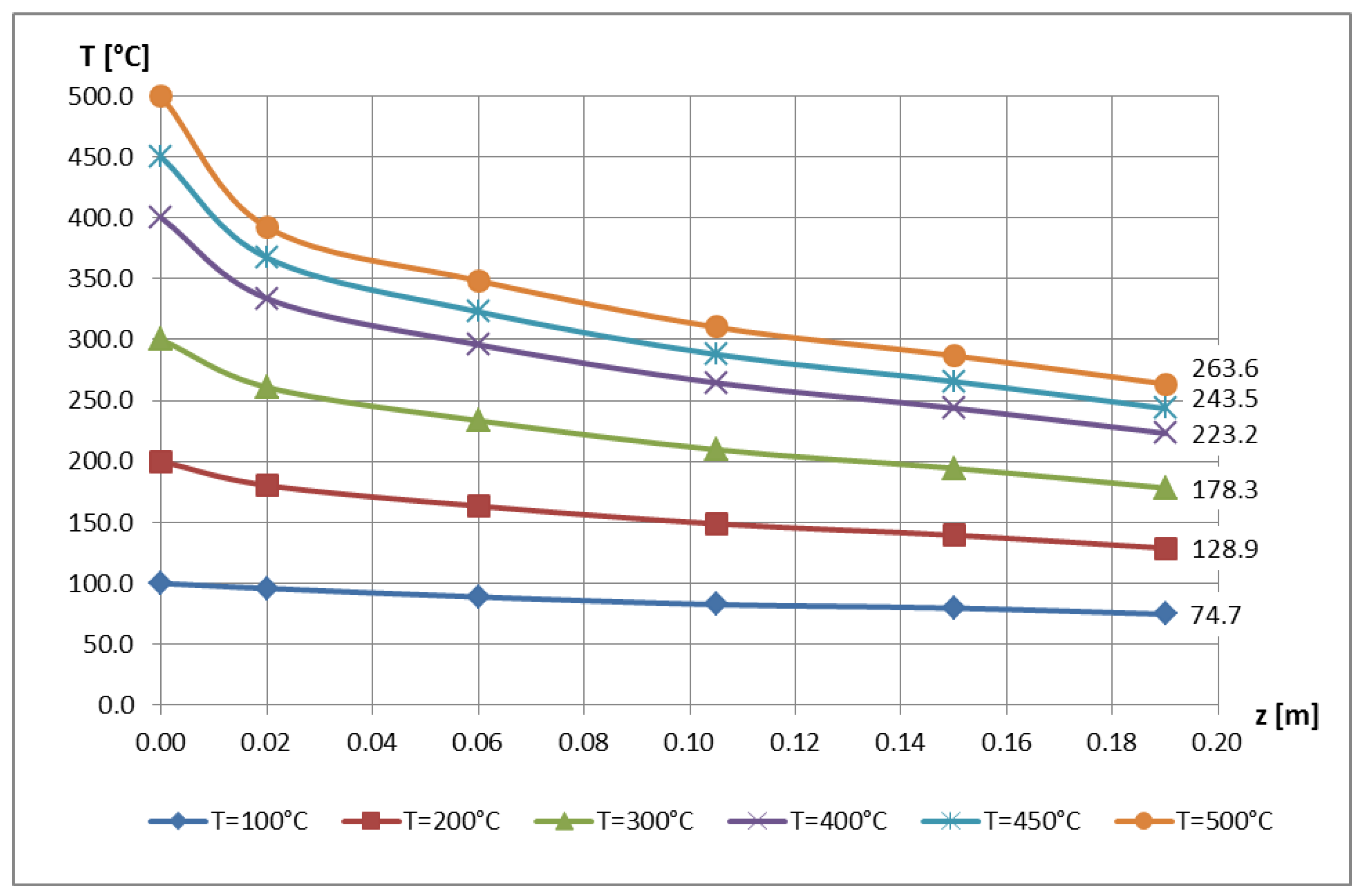
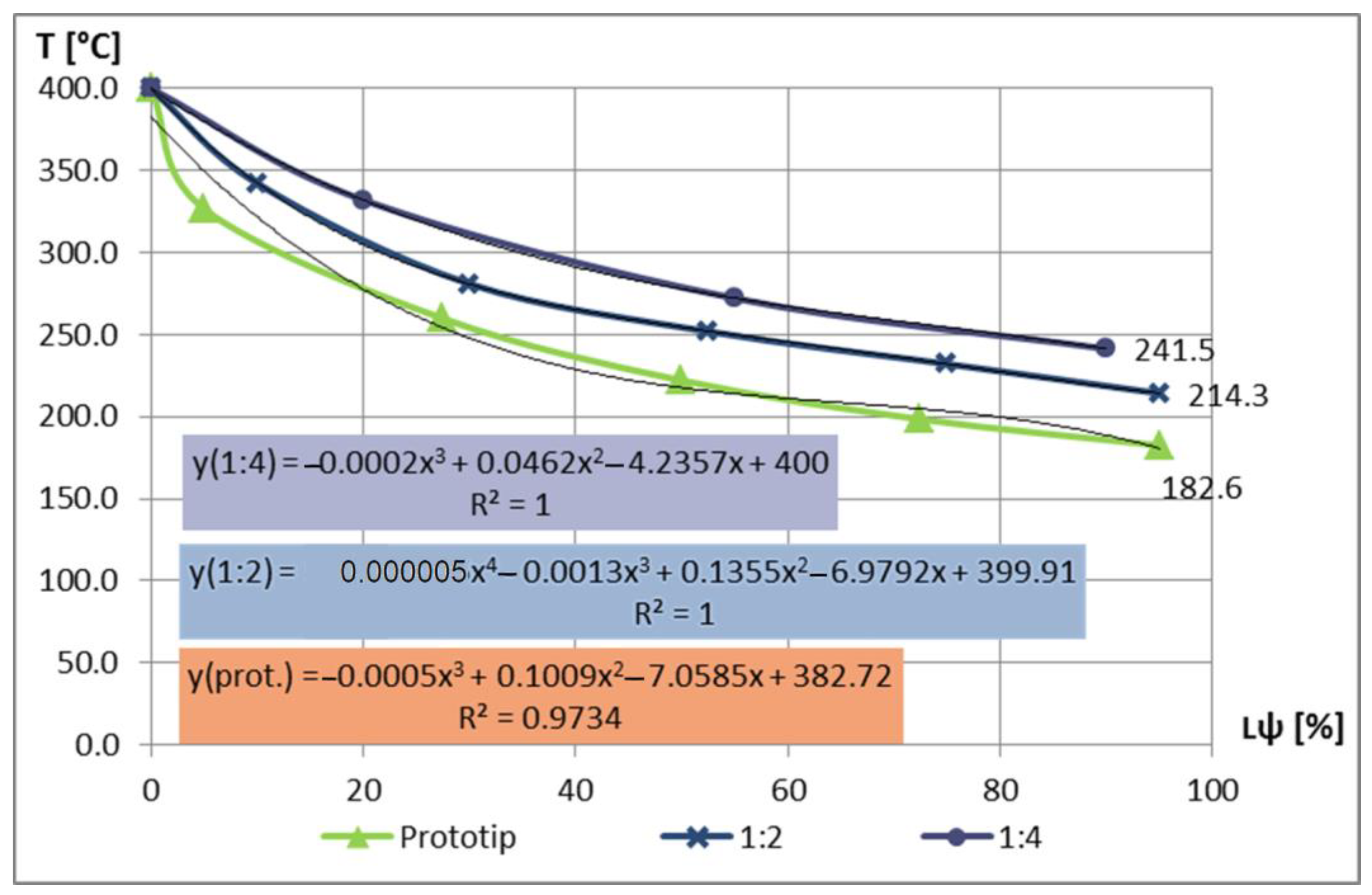
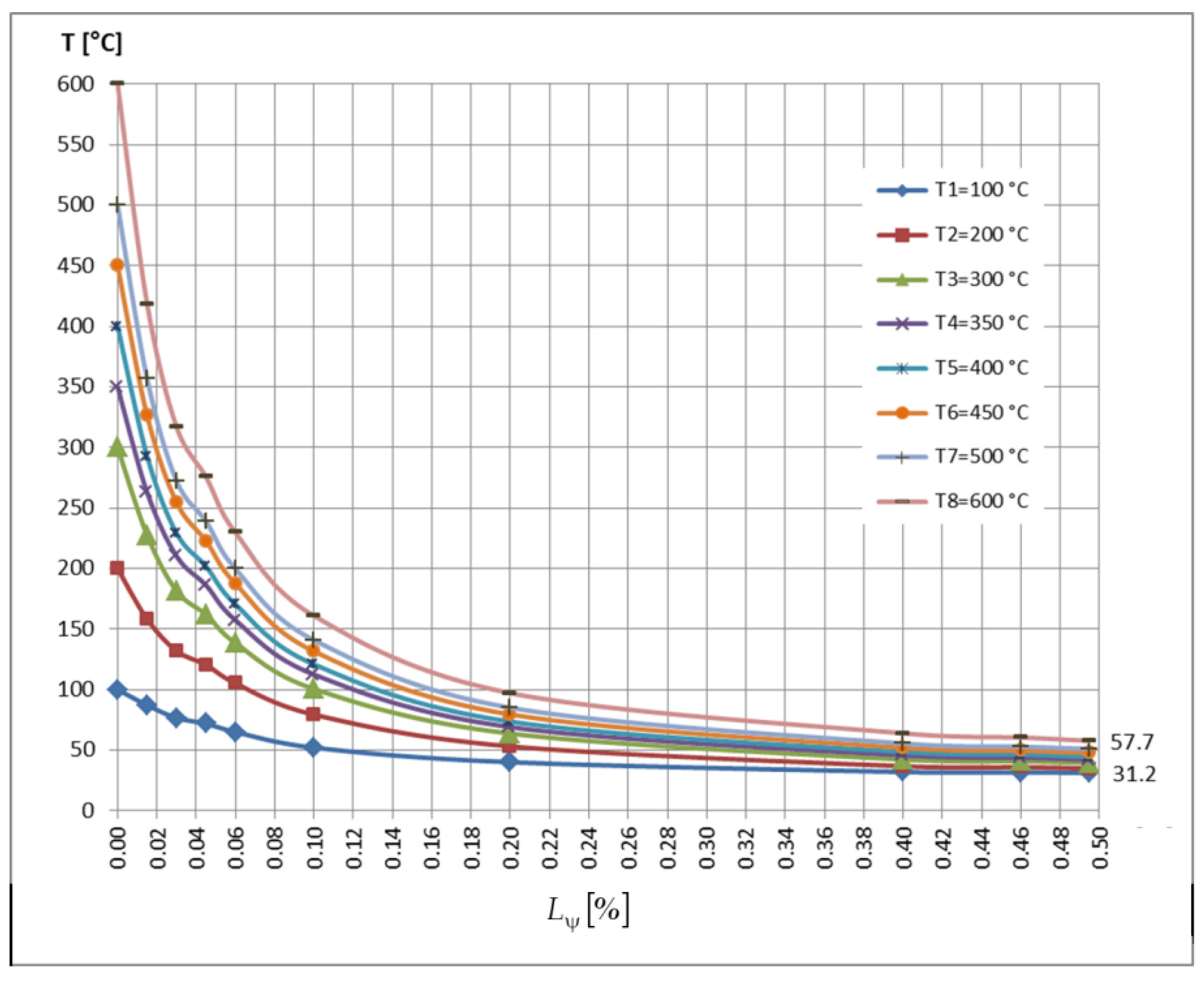
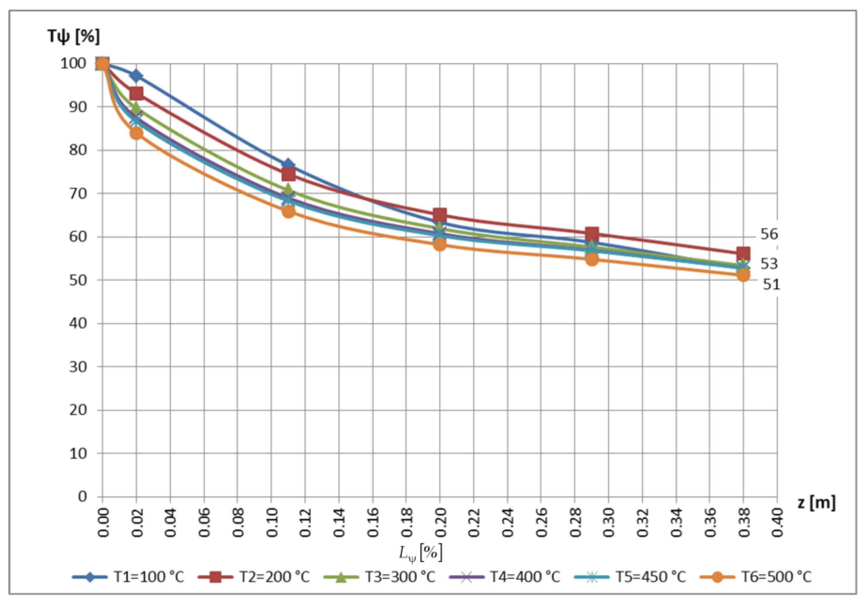
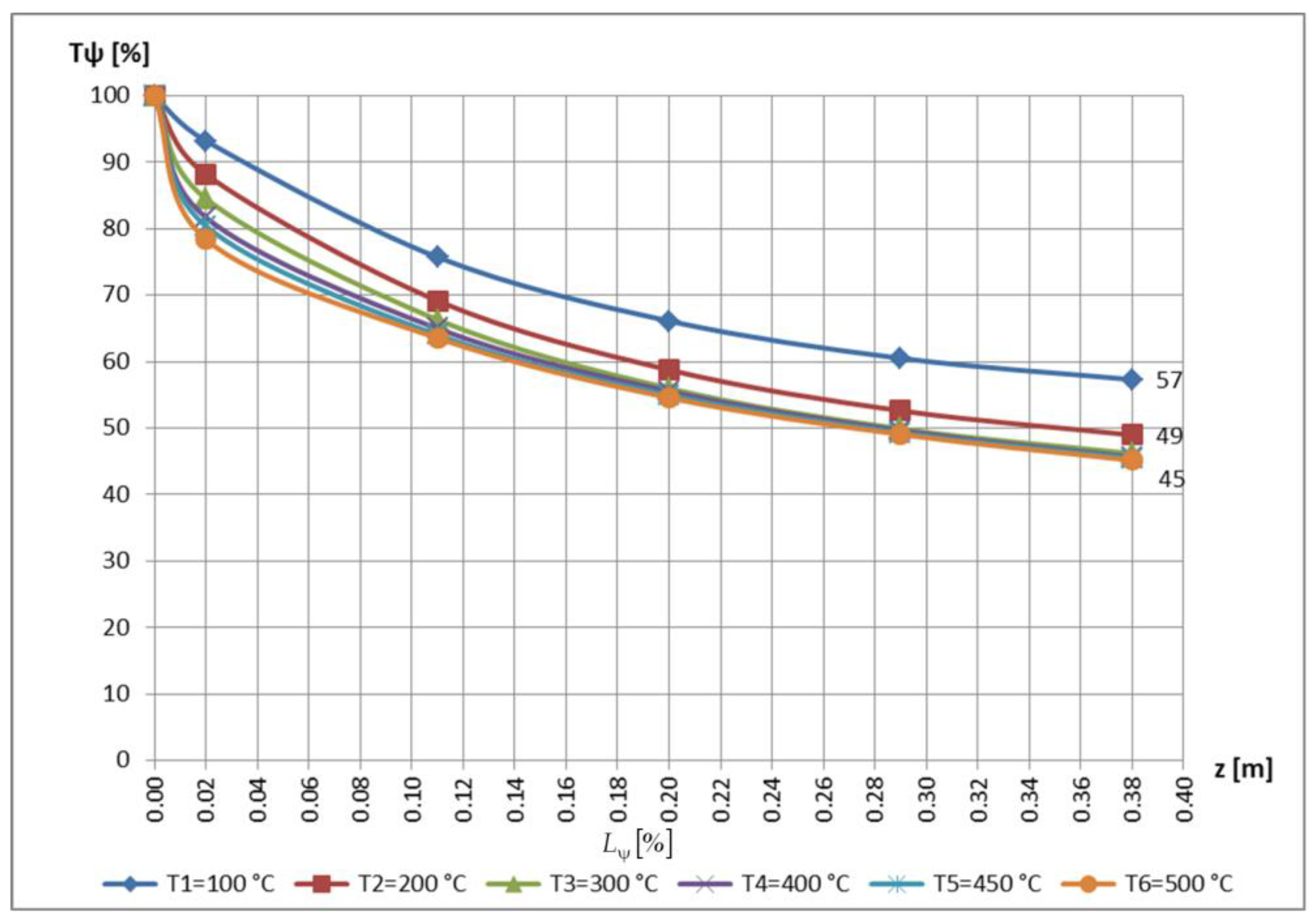
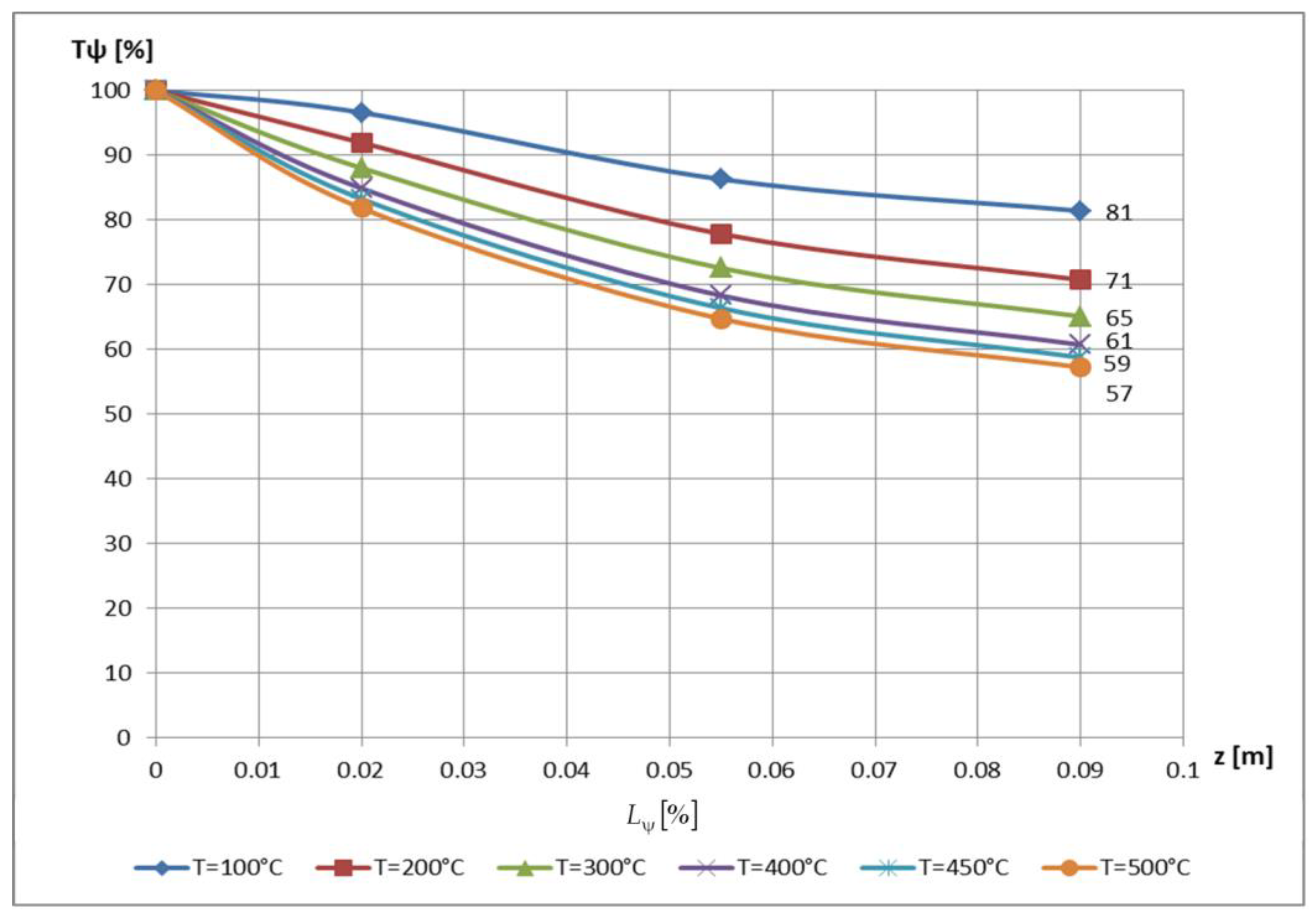
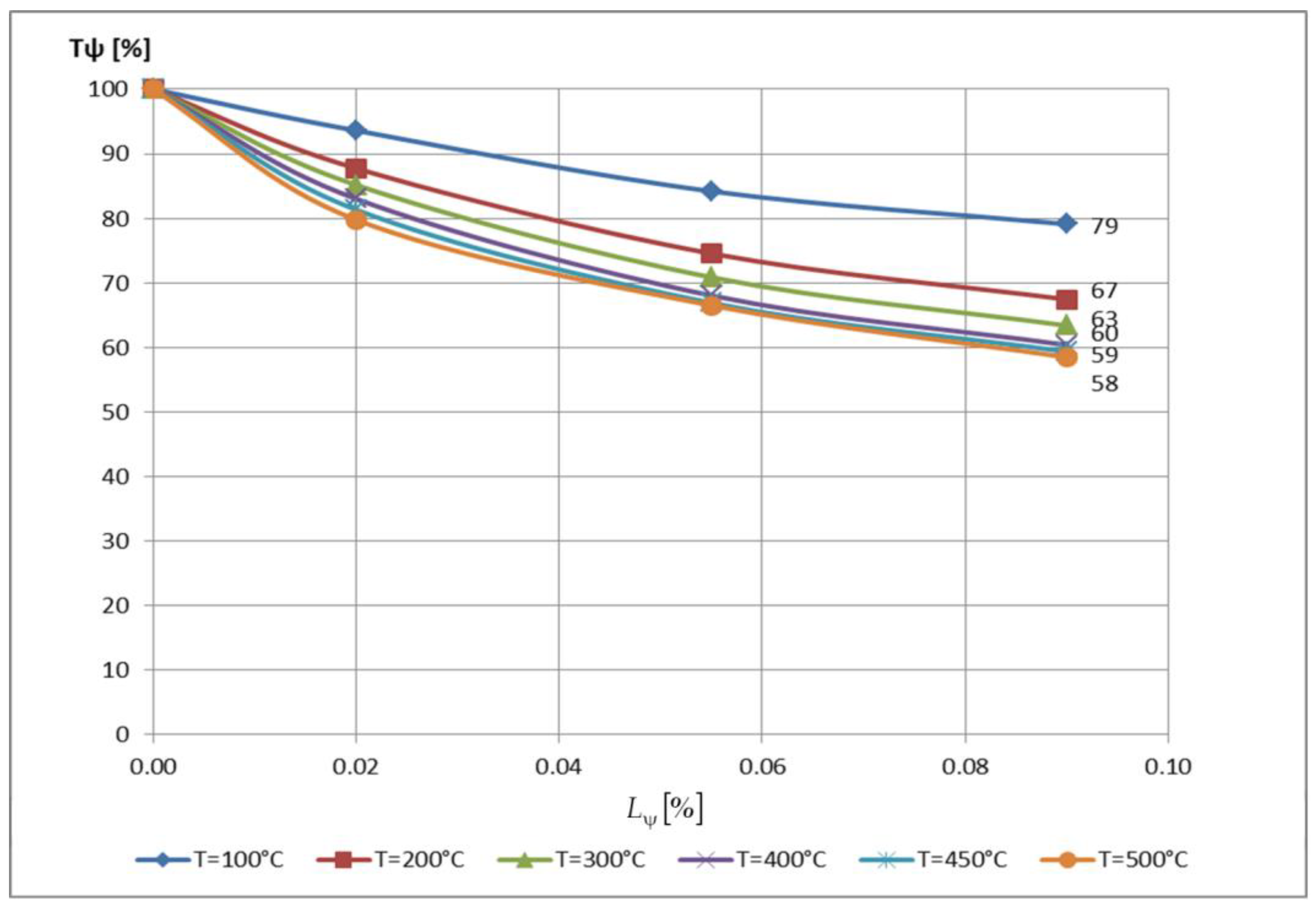
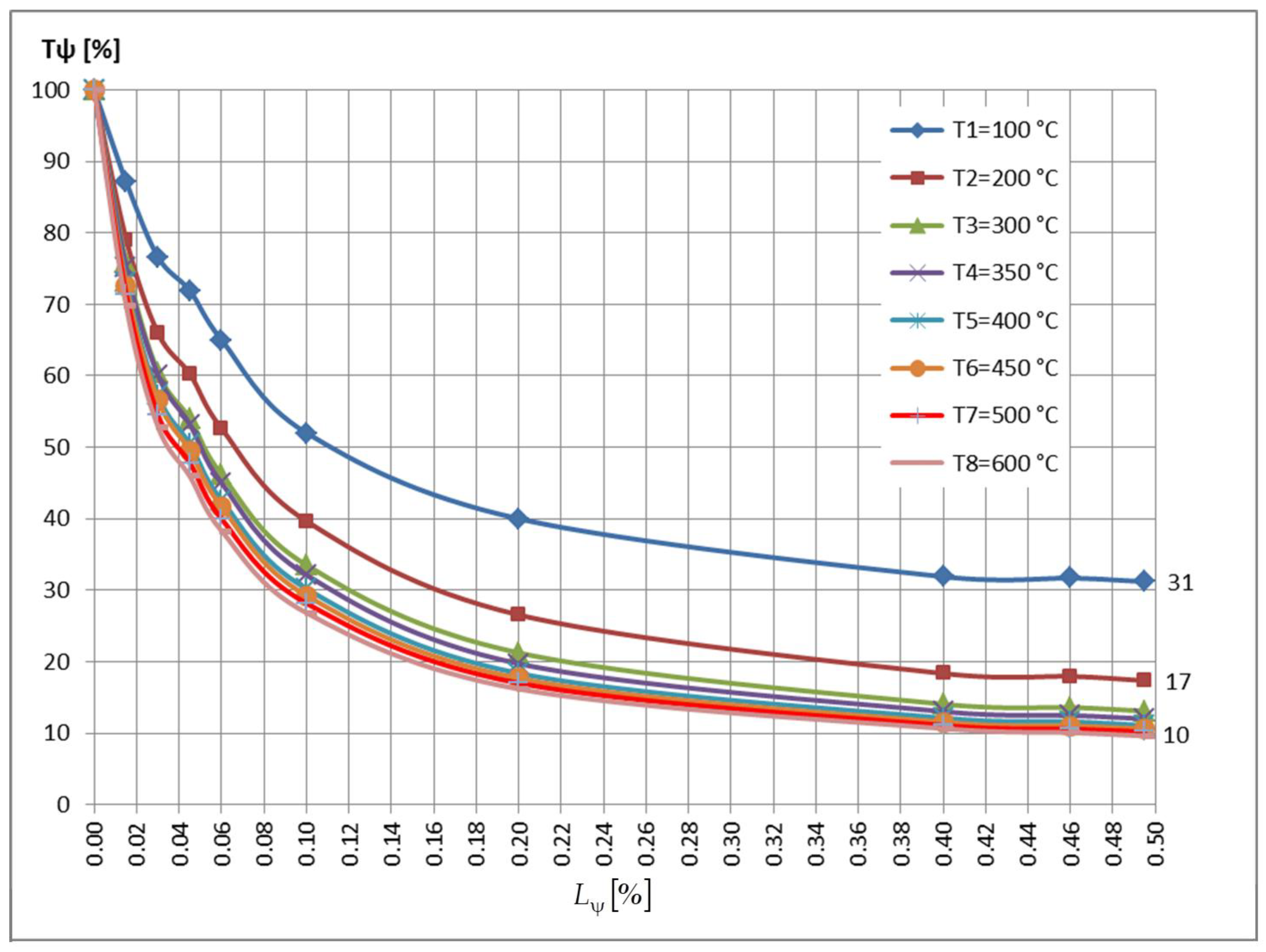
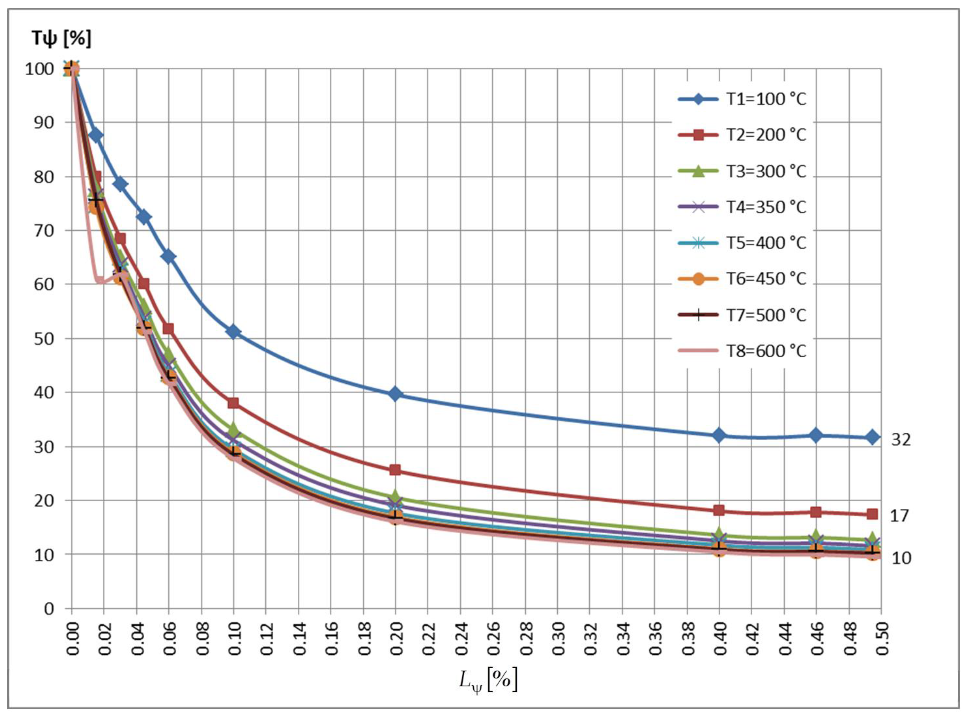
- The greatest gradient for the is on the first interval , where the obtained gradient is 100 %, that will decrease to 62.3 %; on the second interval , there will be a decrease from 62.3 % to 57 %, as well as on the third interval , which will decrease from 57 % to 36.8 %;
- Taking into consideration that represents, in fact, 90 % of the whole bar length , the corresponding gradient correlated with its real length is very small;
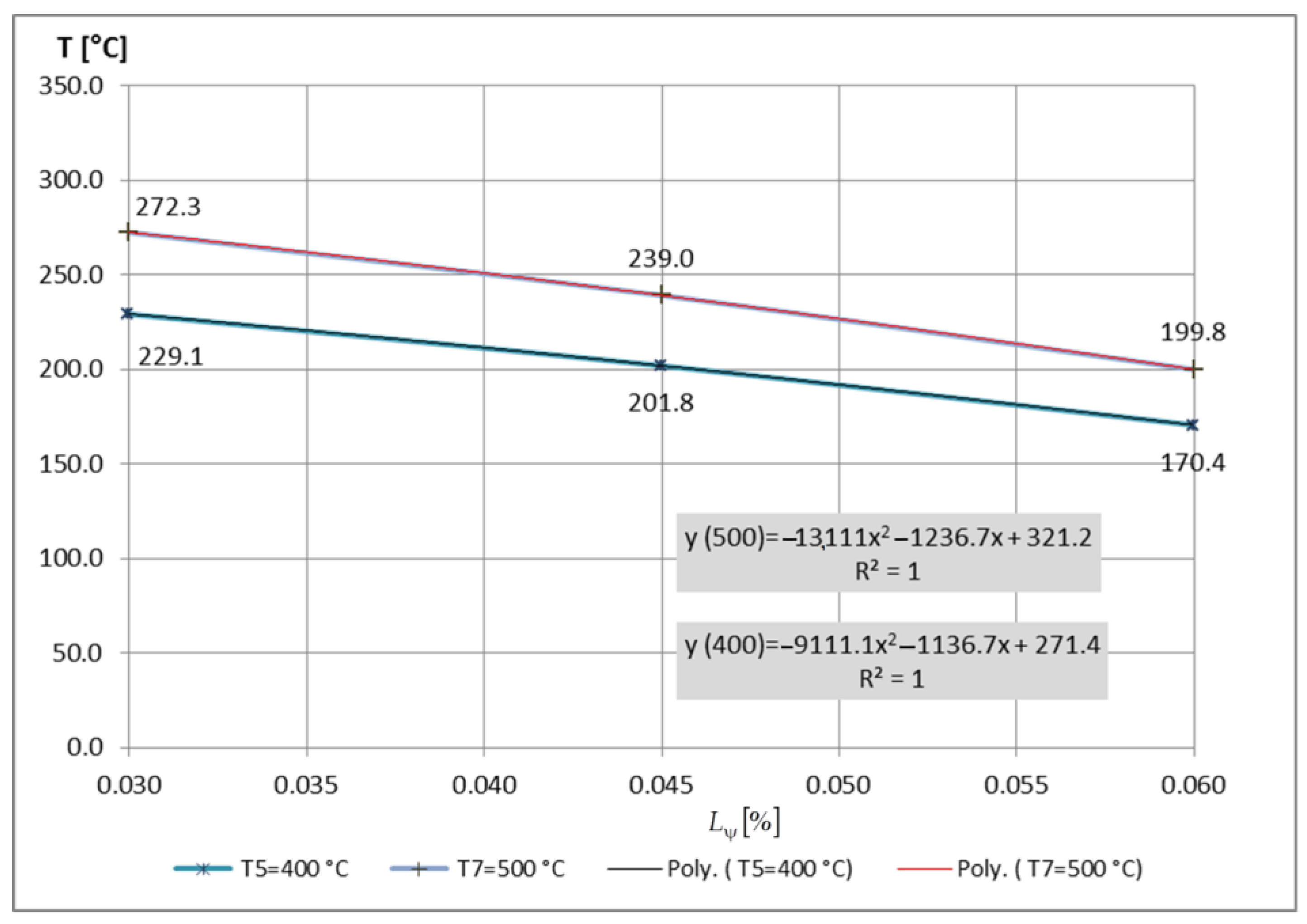
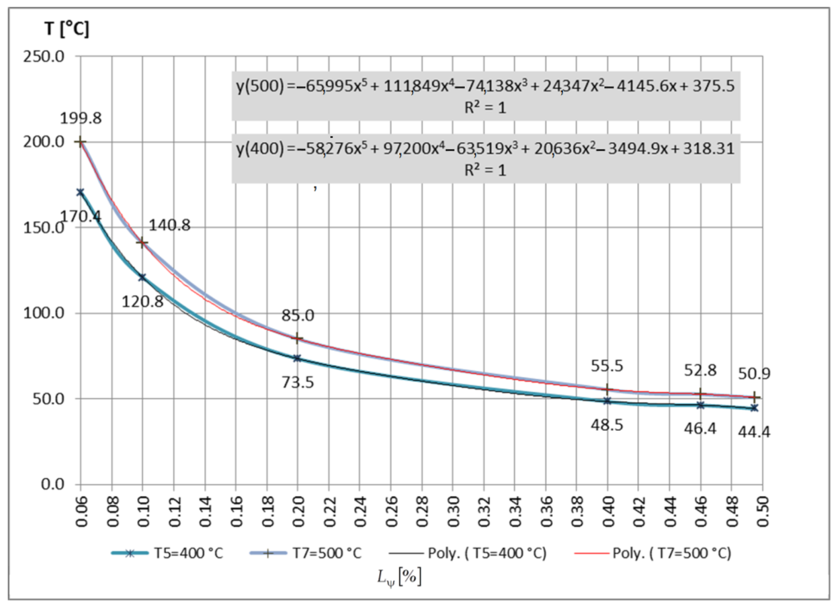
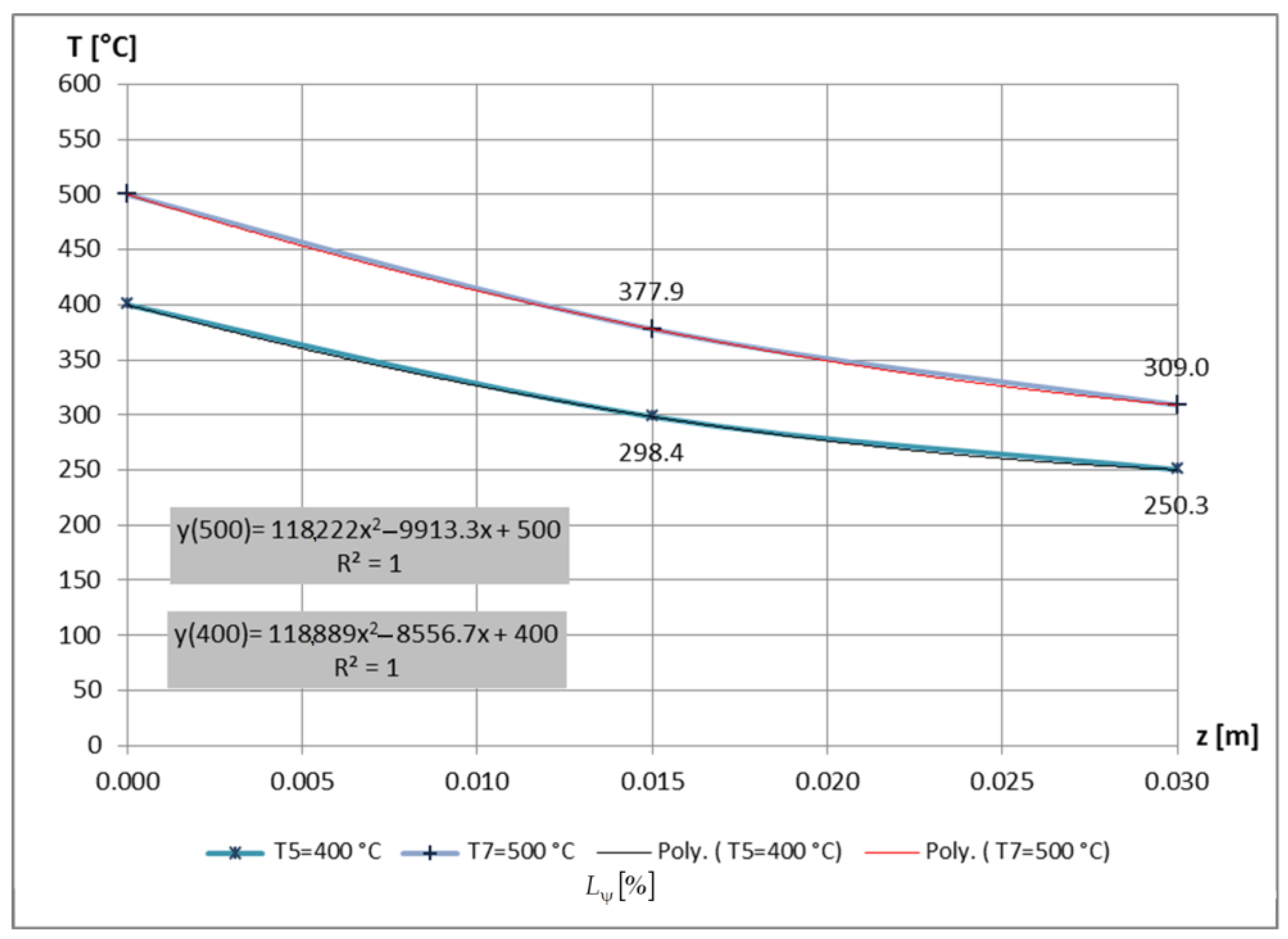
- For other nominal temperatures, the mentioned calculi of can be performed in a similar manner, which can assure, without difficult analytical calculi, that predictable values for the “m” parameter are obtained;
- In the authors’ opinion, these new practical approaches to the temperature distribution law can be applied successfully in the thermal analysis of 2D and 3D structures, in the first stage on reduced scale models, involving the results of the modern dimensional analysis (MDA) (analyzed briefly in the following), as well as in real-scale structures;
- The performed analytical calculi offer a useful tool for fire safety engineers to predict both the heat transfer along the steel structural elements and their load bearing capacity.
- GA works only with a limited number of laws, based on the identification of points, angles and homologous surfaces of the prototype, in accordance with the related model;
- TS provides an extension of these laws, but can also only be applied to a number of particular cases;
- CDA, although theoretically it would be the ideal method of approach, presents several other shortcomings, such as:
- o
- The deduction of the model law (ML) is based on the processing of a limited number of differential equations related to the phenomenon;
- o
- This processing is unfortunately quite arbitrary, non-unitary, and its efficiency depends to a large extent on the user’s experience, usually consisting of grouping some terms of the equations involved, or identifying adimensional groups from the same constitutive equations, in order to obtain dimensionless expressions;
- o
- It requires deep knowledge of higher mathematics, but also of the field of the respective phenomenon;
- o
- Only in particular cases can it provide the complete set of dimensionless variables, based on which the ML is later defined;
- o
- The method, not being unitary in approach, is not easily applicable to ordinary researchers, remaining accessible only to a narrow segment of established specialists.
- The method is unitary, simple and accessible to any researcher;
- It does not require thorough knowledge in the field, but only that all the parameters are taken into account, which can in a certain way have an influence on the respective phenomenon;
- The parameters, which have no influence on the phenomenon, are automatically removed from the protocol;
- The complete set of dimensionless variables is always provided, and consequently also the complete ML;
- The developed method is very flexible, allowing, based on the ML deduced for the general case, customizations to be made in order to simplify and optimize the model, as well as the related experiments;
- MDA allows choosing at will the set of variables that define the protocol of experiments on the model, but also the model itself.
2. Materials and Methods
3. Results
4. Discussion
5. Conclusions
Author Contributions
Funding
Data Availability Statement
Acknowledgments
Conflicts of Interest
References
- Turzó, G. Temperature distribution along a straight bar sticking out from a heated plane surface and the heat flow transmitted by this bar (I)-Theoretical Approach. Ann. Fac. Eng. Hunedoara-Int. J. Eng. 2016, 14, 49–53. [Google Scholar]
- Turzó, G.; Száva, I.R.; Gálfi, B.P.; Száva, I.; Vlase, S.; Hota, H. Temperature Distribution of the Straigth Bar, fixed into a Heated Plane Surface. Fire Mater. 2018, 42, 202–212. [Google Scholar] [CrossRef]
- Turzó, G.; Száva, I.R.; Dancsó, S.; Száva, I.; Vlase, S.; Munteanu, V.; Gălățanu, T.; Asztalos, Z. A New Approach in Heat Transfer Analysis: Reduced-Scale Straight Bars with Massive and Square-Tubular Cross-Sections. Mathematics 2022, 10, 3680. [Google Scholar] [CrossRef]
- Baker, W.; Westine, P.S.; Dodge, F.T. Similarity Methods in Engineering Dynamics; Elsevier: Amsterdam, The Netherlands, 1991. [Google Scholar]
- Barenblatt, G.I. Dimensional Analysis; Gordon and Breach: New York, NY, USA, 1987. [Google Scholar]
- Barr, D.I.H. Consolidation of Basics of Dimensional Analysis. J. Eng. Mech.-ASCE 1984, 110, 1357–1376. [Google Scholar] [CrossRef]
- Bejan, A. Convection Heat Transfer; John Wiley & Sons: Hoboken, NJ, USA, 2013. [Google Scholar]
- Bhaskar, R.; Nigam, A. Qualitative Physics using Dimensional Analysis. Artif. Intell. 1990, 45, 73–111. [Google Scholar] [CrossRef]
- Bridgeman, P.W. Dimensional Analysis; Yale University Press: New Haven, CT, USA, 1922; (Reissued in paperbound in 1963). [Google Scholar]
- Buckingham, E. On Physically Similar Systems. Phys. Rev. 1914, 4, 345. [Google Scholar] [CrossRef]
- Canagaratna, S.G. Is dimensional analysis the best we have to offer. J. Chem. Educ. 1993, 70, 40–43. [Google Scholar] [CrossRef]
- Carabogdan, G.I.; Badea, A.; Brătianu, C.; Muşatescu, V. Methods of Analysis of Thermal Energy Processes and Systems; Technical Publishing House: Bucharest, Romania, 1989. (In Romanian) [Google Scholar]
- Carinena, J.F.; Santander, M. Dimensional Analysis. Adv. Electron. Electron Phys. 1988, 72, 181–258. [Google Scholar]
- Carlson, D.E. Some New Results in Dimensional Analysis. Arch. Ration. Mech. Anal. 1978, 68, 191–210. [Google Scholar] [CrossRef]
- Carslaw, H.S.; Jaeger, J.C. Conduction of Heat in Solid, 2nd ed.; Oxford Science Publications: New York, NY, USA, 1986. [Google Scholar]
- Chen, W.K. Algebraic Theory of Dimensional Analysis. J. Frankl. Inst. 1971, 292, 403–409. [Google Scholar] [CrossRef]
- Coyle, R.G.; Ballicolay, B. Concepts and Software for Dimensional Analysis in Modelling. IEEE Trans. Syst. Man Cybern. 1984, 14, 478–487. [Google Scholar] [CrossRef]
- Fourier, J. Theorie Analytique de la Chaleur; Firmin Didot: Paris, France, 1822. (In French) [Google Scholar]
- Gibbings, J.C. Dimensional Analysis. J. Phys. A-Math. Gen. 1980, 13, 75–89. [Google Scholar] [CrossRef]
- Gibbings, J.C. A Logic of Dimensional Analysis. J. Phys. A-Math. Gen. 1982, 15, 1991–2002. [Google Scholar] [CrossRef]
- Incropera, F.P.; DeWitt, D.P.; Bergman, T.L.; Lavine, A.S. Fundamentals of Heat and Mass Transfer; John Wiley & Sons Ltd.: Chichester, UK, 2002. [Google Scholar]
- Jofre, L.; del Rosario, Z.R.; Iaccarino, G. Data-driven dimensional analysis of heat transfer in irradiated particle-laden turbulent flow. Int. J. Multiph. Flow 2020, 125, 103198. [Google Scholar] [CrossRef]
- Környey, T. Heat Transfer; Műegyetemi Kiadó: Budapest, Hungary, 1999. (In Hungarian) [Google Scholar]
- Langhaar, H.L. Dimensional Analysis and Theory of Models; John Wiley & Sons Ltd.: New York, NY, USA, 1951. [Google Scholar]
- Martins, R.D.A. The Origin of Dimensional Analysis. J. Frankl. Inst. 1981, 311, 331–337. [Google Scholar] [CrossRef]
- Nakla, M. On fluid-to-fluid modeling of film boiling heat transfer using dimensional analysis. Int. J. Multiph. Flow 2011, 37, 229–234. [Google Scholar] [CrossRef]
- Nezhad, A.H.; Shamsoddini, R. Numerical Three-Dimensional Analysis of the Mechanism of Flow and Heat Transfer in a Vortex Tube. Therm. Sci. 2009, 13, 183–196. [Google Scholar] [CrossRef]
- Pankhurst, R.C. Dimensional Analysis and Scale Factor; Chapman & Hall Ltd.: London, UK, 1964. [Google Scholar]
- Quintier, G.J. Fundamentals of Fire Phenomena; John Wiley & Sons: New York, NY, USA, 2006. [Google Scholar]
- Remillard, W.J. Applying Dimensional Analysis. Am. J. Phys. 1983, 51, 137–140. [Google Scholar] [CrossRef]
- Romberg, G. Contribution to Dimensional Analysis. Inginieur Arch. 1985, 55, 401–412. [Google Scholar] [CrossRef]
- Schnittger, J.R. Dimensional Analysis in Design. Journal of Vibration, Accoustic. Stress Reliab. Des.-Trans. ASME 1988, 110, 401–407. [Google Scholar] [CrossRef]
- Sedov, I.L. Similarity and Dimensional Methods in Mechanics; MIR Publisher: Moscow, Russia, 1982. [Google Scholar]
- de Silva, V.P. Determination of the temperature of thermally unprotected steel members under fire situations considerations on the section factor. Lat. Am. J. Solids Struct. 2006, 3, 113–125. [Google Scholar]
- Szekeres, P. Mathematical Foundations of Dimensional Analysis and the Question of Fundamental Units. Int. J. Theor. Phys. 1978, 17, 957–974. [Google Scholar] [CrossRef]
- Șova, M.; Șova, D. Thermotechnics; Transilvania University Press: Brașov, Romania, 2001; Volume II. [Google Scholar]
- Șova, D. Heat Engineering; Transilvania University Press: Brasov, Romania, 2006; ISBN 9789736357664. [Google Scholar]
- Șova, D. Applied Thermodynamics; Transilvania University Press: Brasov, Romania, 2015; ISBN 9786061907144. [Google Scholar]
- Ştefănescu, D.; Marinescu, M.; Dănescu, A. Heat Transfer in Technique; Tehnică: Bucureşti, Romania, 1982; Volume I. [Google Scholar]
- VDI. VDI-Wärmeatlas, 7th ed.; Verein Deutscher Ingenieure: Düsseldorf, Germany, 1994. [Google Scholar]
- Zierep, J. Similarity Laws and Modelling; Marcel Dekker: New York, NY, USA, 1971. [Google Scholar]
- Aglan, A.A.; Redwood, R.G. Strain-Hardening Analysis of Beams with 2 WEB- Rectangular Holes. Arab. J. Sci. Eng. 1987, 12, 37–45. [Google Scholar]
- Al-Homoud, M.S. Performance characteristics and practical applications of common building thermal insulation materials. Build. Environ. 2005, 40, 353–366. [Google Scholar] [CrossRef]
- Bączkiewicz, J.; Malaska, M.; Pajunen, S.; Heinisuo, M. Experimental and numerical study on temperature distribution of square hollow section joints. J. Constr. Steel Res. 2018, 142, 31–43. [Google Scholar] [CrossRef]
- Bailey, C. Indicative fire tests to investigate the behaviour of cellular beams protected with intumescent coatings. Fire Saf. J. 2004, 39, 689–709. [Google Scholar] [CrossRef]
- Ferraz, G.; Santiago, A.; Rodrigues, J.P.; Barata, P. Thermal Analysis of Hollow Steel Columns Exposed to Localized Fires. Fire Technol. 2016, 52, 663–681. [Google Scholar] [CrossRef]
- Franssen, J.-M. Calculation of temperature in fire-exposed bare steel structures: Comparison between ENV 1993-1-2 and EN 1993-1-2. Fire Saf. J. 2006, 41, 139–143. [Google Scholar] [CrossRef]
- Franssen, J.-M.; Real, P.V. Fire Design of Steel Structures, ECCS Eurocode Design Manuals, ECCS-European Convention for Constructional Steelwork; Ernst & Sohn: Berlin, Germany, 2010. [Google Scholar]
- Gao, F.; Guan, X.-Q.; Zhu, H.P.; Liu, X.-N. Fire resistance behaviour of tubular T-joints reinforced with collar plates. J. Constr. Steel Res. 2015, 115, 106–120. [Google Scholar] [CrossRef]
- Ghojel, J.I.; Wong, M.B. Heat transfer model for unprotected steel members in a standard compartment fire with participating medium. J. Constr. Steel Res. 2005, 61, 825–833. [Google Scholar] [CrossRef]
- Xiao, B.Q.; Li, Y.P.; Long, G.B. A Fractal Model of Power-Law Fluid through Charged Fibrous Porous Media by using the Fractional-Derivative Theory. FRACTALS- Complex Geom. Patterns Scaling Nat. Soc. 2022, 30, 2250072. [Google Scholar] [CrossRef]
- Xiao, B.Q.; Fang, J.; Long, G.B.; Tao, Y.Z.; Huang, Z.J. Analysis of Thermal Conductivity of Damaged Tree-Like Bifurcation Network with Fractal Roughened Surfaces. FRACTALS-Complex Geom. Patterns Scaling Nat. Soc. 2022, 30, 2250104. [Google Scholar] [CrossRef]
- Long, G.; Liu, Y.; Xu, W.; Zhou, P.; Zhou, J.; Xu, G.; Xiao, B. Analysis of Crack Problems in Multilayered Elastic Medium by a Consecutive Stiffness Method. Mathematics 2022, 10, 4403. [Google Scholar] [CrossRef]
- Kado, B.; Mohammad, S.; Lee, Y.H.; Shek, P.N.; Ab Kadir, M.A. Temperature Analysis of Steel Hollow Column Exposed to Standard Fire. J. Struct. Technol. 2018, 3, 1–8. [Google Scholar]
- Khan, M.A.; Shah, I.A.; Rizvi, Z.; Ahmad, J. A numerical study on the validation of thermal formulations towards the behaviours of RC beams. Sci. Mater. Today Proc. 2019, 17, 227–234. [Google Scholar] [CrossRef]
- Krishnamoorthy, R.R.; Bailey, C.G. Temperature distribution of intumescent coated steel framed connection at elevated temperature. In Proceedings of the Nordic Steel Construction Conference ‘09, Malmo, Sweden, 2–4 September 2009; Swedish Institute of Steel Construction: Stockholm, Sweden, 2009. Publication 181. Volume I, pp. 572–579. [Google Scholar]
- Lawson, R.M. Fire engineering design of steel and composite Buildings. J. Constr. Steel Res. 2001, 57, 1233–1247. [Google Scholar] [CrossRef]
- Levac, M.L.J.; Soliman, H.M.; Ormiston, S.J. Three-dimensional analysis of fluid flow and heat transfer in single- and two-layered micro-channel heat sinks. Heat Mass Transf. 2011, 47, 1375–1383. [Google Scholar] [CrossRef]
- Noack, J.; Rolfes, R.; Tessmer, J. New layerwise theories and finite elements for efficient thermal analysis of hybrid structures. Comput. Struct. 2003, 81, 2525–2538. [Google Scholar] [CrossRef]
- Papadopoulos, A.M. State of the art in thermal insulation materials and aims for future developments. Energy Build. 2005, 37, 77–86. [Google Scholar] [CrossRef]
- Tafreshi, A.M.; Di Marzo, M. Foams and gels as temperature protection agents. Fire Saf. J. 1999, 33, 295–305. [Google Scholar] [CrossRef]
- Yang, K.-C.; Chen, S.J.; Lin, C.-C.; Lee, H.-H. Experimental study on local buckling of fire-resisting steel columns under fire load. J. Constr. Steel Res. 2005, 61, 553–565. [Google Scholar] [CrossRef]
- Yang, J.; Shao, Y.B.; Chen, C. Experimental study on fire resistance of square hollow section (SHS) tubular T-joint under axial compression. Adv. Steel Constr. 2014, 10, 72–84. [Google Scholar]
- Wong, M.B.; Ghojel, J.I. Sensitivity analysis of heat transfer formulations for insulated structural steel components Fire. Saf. J. 2003, 38, 187–201. [Google Scholar] [CrossRef]
- Vlase, S.; Teodorescu-Draghicescu, H.; Calin, M.R.; Scutaru, M.L. Advanced Polylite composite laminate material behavior to tensile stress on weft direction. J. Optoelectron. Adv. Mater. 2022, 14, 658–663. [Google Scholar]
- Alshqirate, A.A.Z.S.; Tarawneh, M.; Hammad, M. Dimensional Analysis and Empirical Correlations for Heat Transfer and Pressure Drop in Condensation and Evaporation Processes of Flow Inside Micropipes: Case Study with Carbon Dioxide (CO2). J. Braz. Soc. Mech. Sci. Eng. 2012, 34, 89–96. [Google Scholar]
- Andreozzi, A.; Bianco, N.; Musto, M.; Rotondo, G. Scaled models in the analysis of fire-structure interaction. In Proceedings of the 33rd UIT (Italian Union of Thermo-Fluid-Dynamics) Heat Transfer Conference, L’Aquila, Italy, 22–24 June 2015; IOP: Bristol, UK, 2015; Volume 655, p. 012053. [Google Scholar] [CrossRef]
- He, S.-B.; Shao, Y.-B.; Zhang, H.-Y.; Wang, Q. Parametric study on performance of circular tubular K-joints at elevated temperature. Fire Saf. J. 2015, 71, 174–186. [Google Scholar] [CrossRef]
- Illan, F.; Viedma, A. Experimental study on pressure drop and heat transfer in pipelines for brine based ice slurry Part II: Dimensional analysis and rheological Model. Int. J. Refrig.-Rev. Int. Du Froid 2009, 32, 1024–1031. [Google Scholar] [CrossRef]
- Gálfi, B.-P.; Száva, I.; Șova, D.; Vlase, S. Thermal Scaling of Transient Heat Transfer in a Round Cladded Rod with Modern Dimensional Analysis. Mathematics 2021, 9, 1875. [Google Scholar] [CrossRef]
- Munteanu (Száva), I.R. Investigation Concerning Temperature Field Propagation along Reduced Scale Modelled Metal Structures. Ph.D. Thesis, Transilvania University of Brasov, Brasov, Romania, 2018. [Google Scholar]
- Száva, I.R.; Șova, D.; Dani, P.; Élesztős, P.; Száva, I.; Vlase, S. Experimental Validation of Model Heat Transfer in Rectangular Hole Beams Using Modern Dimensional Analysis. Mathematics 2022, 10, 409. [Google Scholar] [CrossRef]
- Șova, D.; Száva, I.R.; Jármai, K.; Száva, I.; Vlase, S. Modern method to analyze the Heat Transfer in a Symmetric Metallic Beam with Hole. Symmetry 2022, 14, 769. [Google Scholar] [CrossRef]
- Trif, I.; Asztalos, Z.; Kiss, I.; Élesztős, P.; Száva, I.; Popa, G. Implementation of the Modern Dimensional Analysis in Engineering Problems; Basic Theoretical Layouts. Ann. Fac. Eng. Hunedoara 2019, 17, 73–76. [Google Scholar]
- Szirtes, T. The Fine Art of Modelling. SPAR J. Eng. Technol. 1992, 1, 37. [Google Scholar]
- Szirtes, T. Applied Dimensional Analysis and Modelling; McGraw-Hill: Toronto, ON, Canada, 1998. [Google Scholar]
- Száva, I.; Szirtes, T.; Dani, P. An Application of Dimensional Model Theory in the Determination of the Deformation of a Structure. Eng. Mech. 2006, 13, 31–39. [Google Scholar]
- Száva, R.I.; Száva, I.; Vlase, S.; Gálfi, P.B.; Jármai, K.; Gălățanu, T.; Popa, G.; Asztalos, Z. Modern Dimensional Analysis-Based Steel Column’ Heat Transfer Evaluation using Multiple Experiments. Symmetry 2022, 14, 1952. [Google Scholar] [CrossRef]
- Dani, P.; Száva, I.R.; Kiss, I.; Száva, I.; Popa, G. Principle Schema of an Original Full-, and Reduced-Scale Testing Bench, Destined to Fire Protection Investigations. Ann. Fac. Eng. Hunedoara-Int. J. Eng. 2018, 16, 149–152. [Google Scholar]
- Gálfi, B.P.; Száva, R.I.; Száva, I.; Vlase, S.; Gălățanu, T.; Jármai, K.; Asztalos, Z.; Popa, G. Modern Dimensional Analysis based on Fire-Protected Steel Members’ Analysis using Multiple Experiments. Fire 2022, 5, 210. [Google Scholar] [CrossRef]


| Prototype, at Scale 1:1 | Model I, at Scale 1:2 | Model II, at Scale 1:4 | |
|---|---|---|---|
| Dimensions, in m | |||
| La | 0.370 | 0.185 | 0.0925 |
| Lb | 0.370 | 0.185 | 0.0925 |
| Lc | 0.006 | 0.003 | 0.0015 |
| Ld | 0.350 | 0.175 | 0.0875 |
| Le | 0.350 | 0.175 | 0.0875 |
| Lf | 0.016 | 0.008 | 0.004 |
| Lg | 0.016 | 0.008 | 0.004 |
| Lh | 0.400 | 0.200 | 0.100 |
| Lk | 0.010 | 0.005 | 0.0025 |
| Lm | 0.450 | 0.450 | 0.450 |
| Ln | 0.450 | 0.450 | 0.450 |
| Prototype, at Scale 1:1 | Model I, at Scale 1:2 | Model II, at Scale 1:4 | Model III, at Scale 1:10 |
|---|---|---|---|
| Coordinates z(j) in m | |||
| 0.020 | 0.020 | 0.020 | 0.015 |
| 0.110 | 0.060 | 0.055 | 0.030 |
| 0.200 | 0.105 | 0.090 | 0.045 |
| 0.290 | 0.150 | 0.060 | |
| 0.380 | 0.190 | 0.100 | |
| 0.200 | |||
| 0.400 | |||
| 0.460 | |||
| 0.495 | |||
Disclaimer/Publisher’s Note: The statements, opinions and data contained in all publications are solely those of the individual author(s) and contributor(s) and not of MDPI and/or the editor(s). MDPI and/or the editor(s) disclaim responsibility for any injury to people or property resulting from any ideas, methods, instructions or products referred to in the content. |
© 2023 by the authors. Licensee MDPI, Basel, Switzerland. This article is an open access article distributed under the terms and conditions of the Creative Commons Attribution (CC BY) license (https://creativecommons.org/licenses/by/4.0/).
Share and Cite
Száva, I.; Vlase, S.; Száva, I.-R.; Turzó, G.; Munteanu, V.M.; Gălățanu, T.; Asztalos, Z.; Gálfi, B.-P. Modern Dimensional Analysis-Based Heat Transfer Analysis: Normalized Heat Transfer Curves. Mathematics 2023, 11, 741. https://doi.org/10.3390/math11030741
Száva I, Vlase S, Száva I-R, Turzó G, Munteanu VM, Gălățanu T, Asztalos Z, Gálfi B-P. Modern Dimensional Analysis-Based Heat Transfer Analysis: Normalized Heat Transfer Curves. Mathematics. 2023; 11(3):741. https://doi.org/10.3390/math11030741
Chicago/Turabian StyleSzáva, Ioan, Sorin Vlase, Ildikó-Renáta Száva, Gábor Turzó, Violeta Mihaela Munteanu, Teofil Gălățanu, Zsolt Asztalos, and Botond-Pál Gálfi. 2023. "Modern Dimensional Analysis-Based Heat Transfer Analysis: Normalized Heat Transfer Curves" Mathematics 11, no. 3: 741. https://doi.org/10.3390/math11030741