Structural Modal Parameter Identification Method Based on the Delayed Transfer Rate Function under Periodic Excitations

Abstract

The dynamic response transfer rate function (TRF) is increasingly used in the field of structural modal parameter identification because it does not depend on the white noise assumption of the excitation. In this paper, the interference of periodic excitation on structural modal parameter identification using TRF is analyzed theoretically for a class of civil engineering structures with obvious periodic components in excitation, and then an identification method of structural real modal parameters is proposed. First, a delayed TRF is constructed, and the pseudo-frequency response function is further obtained to identify the periodic spurious poles of the whole system. Then, the effective identification of the real modal parameters of the structure is achieved by comparing the system poles identified via conventional TRF. Finally, the feasibility and robustness of the proposed method were verified using a calculation example with four-degrees-of-freedom system. In addition, the modal parameters of a structure under periodic excitation were effectively identified by taking a pumping station as an example, and the results show that the method accurately identified the structural modal parameters when the excitation contained periodic components, which has wider prospects for technical applications.

1. Introduction

In large civil engineering projects, the modal parameters of a structure are important pieces of information reflecting the dynamic characteristics of the structure, and accurate recording of the modal parameters is a prerequisite for effective structural health evaluation and damage diagnosis [1,2,3]. The operating modal analysis method can effectively obtain the modal parameters of a structure without affecting the normal operation of the structure, based only on the dynamic response of the structure under the environmental excitation [4,5]. Its low cost of operation and harmlessness to structures have led to its development as an effective tool for structural modal analysis of large civil engineering projects [6,7,8]. It is worth noting that the modal analysis method based on the transfer rate function (TRF) is an emerging method of structural operational modal analysis developed in recent decades which does not depend on the white noise excitation assumption of the load, greatly expands the scope of engineering applications of the operational modal analysis, and has received wide attention [9,10,11]. The commonly used TRFs take the form of response transmissibility [12,13] and power spectral density transmissibility of the structure [14]. According to the nature of the TRF intersection at the system poles, the identification of the modal parameters can be achieved by constructing the quasi-frequency response function matrix of the structure [15].

As mentioned above, the TRF has special properties. Devriendt et al. [16] successfully identified the modal parameters of a pedestrian bridge, extended the scalar transmissibility to the transmissibility matrix, and proposed a multivariate transmissibility [17] and pseudo-transmissibility [18] method for operational modal analysis. Weitjens et al. [19] proposed a transmissibility operational modal analysis method for multiple-input–multiple-output systems using multi-reference-point least-squares complex frequency domain estimation to solve for the system poles and derive the system modal parameters based on the steady-state diagram. Zhang et al. [20] constructed rational functions by applying transmissibility for two different loading cases and identified the modal parameters using orthogonal polynomial fitting. Araujo et al. [21] used a combination of transmissibility and blind source separation techniques to analyze structural modes for a low signal-to-noise ratio, mode-dense case. Li et al. [22] applied the vibration response transmissibility to analyze structural operating modes. It can be seen that the TRF has been widely used in the modal identification of various civil engineering structures.

In industrial plants, hydraulic (thermal) powerhouses, and other types of engineering structure, the ambient excitation contains an obvious cyclical component that is subject to the influence of rotating mechanical equipment during operation. Conventional modal analysis methods for TRFs do not account for the presence of significant periodic components in the ambient excitation [23], making it difficult to effectively identify false modes introduced by periodic excitation. Simultaneously, the periodic load components of such structures have a high energy proportion, which tends to obscure the real modal information of the structure [24]. In addition, there are some methods to identify false modes, such as sparse decomposition techniques and statistical methods [25], methods based on fuzzy clustering [26], and modal order-determination indexes [27]. Although some attempts have been made to address this issue, these methods still struggle to accurately identify the false modes introduced by periodic excitation [28].

For this purpose, based on analysis of the mechanism of the influence of periodic excitation on modal identification, this paper proposes identification of the false modes introduced by periodic excitation by establishing a delayed TRF. Simultaneously, the conventional TRF modal recognition method is combined to identify the real poles of the system to effectively obtain the real modal parameters of the structure. Finally, it was verified that the method is effective in identifying the real modal parameters of a structure when the ambient excitation contains a periodic component, and that the method has good applicability at various amplitudes and frequencies of periodic excitation, using a technical calculation example of a four-degrees-of-freedom (4-DOF) system.

The remainder of this paper is organized as follows. The basic theories of modal parameter identification, the periodic excitation effect, and the delayed TRF method are presented in Section 2. The example analysis of this study, including the numerical calculation of a 4-DOF system and modal parameter identification of a pumping station, is described in Section 3. Finally, the conclusions are given in Section 4.

2. Basic Theories

2.1. Modal Parameter Identification Based on Acceleration TRF

For a viscous damping system with N degrees of freedom, the forced vibration equation is written as follows:

$$M\ddot{y}\left(t\right)+C\dot{y}\left(t\right)+Ky\left(t\right)=f\left(t\right)$$

(1)

where M, C, and K are the matrices of mass, damping, and stiffness, respectively; $f\left(t\right)$ is the excitation vector; and $y\left(t\right)$ is the displacement response vector.

Under the condition that the initial system states are 0 and the system excitation is smooth, the Laplace transformation of Equation (1) yields

$$Y\left(s\right)=H\left(s\right)F\left(s\right)={\displaystyle {\sum }_{k=1}^Q{H}_k\left(s\right)}{F}_k\left(s\right)$$

(2)

where $Y\left(s\right)$ and $F\left(s\right)$ are the Laplace transformations of $y\left(t\right)$ and $f\left(t\right)$, respectively; s is the Laplace variable; $H\left(s\right)$ is the transfer function matrix of the system, $H\left(s\right)={\left(s^{2}M+sC+K\right)}^{-1}$; Q is the number of load degrees of freedom; and $H_k\left(s\right)$ is the row vector in $H\left(s\right)$ corresponding to the load degrees of freedom k.

The acceleration response TRF $t_{ij}^A\left(s\right)$ is defined as the ratio of the acceleration response of degrees of freedom i and j in the Laplace domain. It can be proven [18] that under the condition that initial displacement and initial velocity are zero, the acceleration transmissibility of the structure is equal to the displacement transmissibility, that is

$$t_{ij}^A\left(s\right)=\frac{A_i\left(s\right)}{A_j\left(s\right)}=t_{ij}^D\left(s\right)=\frac{Y_i\left(s\right)}{Y_j\left(s\right)}=\frac{{\displaystyle {\sum }_{k=1}^Q{H}_{ik}\left(s\right)F_k\left(s\right)}}{{\displaystyle {\sum }_{k=1}^Q{H}_{jk}\left(s\right)F_k\left(s\right)}}$$

(3)

where $Y_i\left(s\right)$ and $A_i\left(s\right)$ denote the Laplace transformations of the displacement response $y_i\left(t\right)$ and acceleration response $a_i\left(t\right)$ of DOF i, respectively. $H_{ik}\left(s\right)$ denotes the i-th row and k-th column element of $H\left(s\right)$.

For the sake of simplicity, the transmissibility of the acceleration response is denoted by $t_{ij}^{}\left(s\right)$ in the following. From the form of Equation (3), it can be stated that the TRF $t_{ij}^{}\left(s\right)$ under multipoint excitation conditions is related to both the system properties $H\left(s\right)$ and the excitation $F\left(s\right)$. Therefore, $t_{ij}^{}\left(s\right)$ differs for different loading conditions.

According to the theory of modal analysis and the residue theorem, the following relationship can be obtained:

$$\underset{s\to {\lambda }_m}{\lim }\left(s-{\lambda }_m\right)H\left(s\right)={\psi }_m{l}_m^T$$

(4)

where ${\lambda }_m$ is the pole of the m-th order mode; ${\psi }_m$ and $l_m^T$ are the vibration vector and the modal participation vector corresponding to ${\lambda }_m$, respectively.

From Equations (3) and (4), the following equation can be obtained when $s\to {\lambda }_m$:

$$\begin{array}{l}\underset{s\to {\lambda }_m}{\lim }{t}_{ij}^{}\left(s\right)=\frac{\underset{s\to {\lambda }_m}{\lim }{\displaystyle {\sum }_{k=1}^Q\left(s-{\lambda }_m\right)H_{ik}\left(s\right)}{F}_k^{}\left(s\right)}{\underset{s\to {\lambda }_m}{\lim }{\displaystyle {\sum }_{k=1}^Q\left(s-{\lambda }_m\right)H_{jk}\left(s\right)}{F}_k^{}\left(s\right)}=\frac{{\displaystyle {\sum }_{k=1}^Q{\psi }_{m,i}{l}_{m,k}}{F}_k^{}\left({\lambda }_m\right)}{{\displaystyle {\sum }_{k=1}^Q{\psi }_{m,j}{l}_{m,k}}{F}_k^{}\left({\lambda }_m\right)}\\ \hspace{1em}\hspace{1em}\hspace{1em}\hspace{1em}=\frac{{\psi }_{m,i}}{{\psi }_{m,j}}\cdot \frac{{\displaystyle {\sum }_{k=1}^Q{l}_{m,k}}{F}_k^{}\left({\lambda }_m\right)}{{\displaystyle {\sum }_{k=1}^Q{l}_{m,k}}{F}_k^{}\left({\lambda }_m\right)}=\frac{{\psi }_{m,i}}{{\psi }_{m,j}}\end{array}$$

(5)

From Equation (5), it can be seen that for any load excitation condition, the TRF $t_{ij}^{}\left(s\right)$ of the system acceleration response at the natural frequency pole ${\lambda }_m$ always remains the same. Based on this property, the identification of structural modal parameters can be carried out.

The acceleration response sequence is divided into $N_f$ periods and the TRF $t_{ij}^{f_k}\left(s\right)$ under each period is calculated separately. By choosing a specific output DOF j and a time period $f_s$, the matrix $TH\left(s\right)$ can be constructed as follows:

$$TH\left(s\right)=\frac{1}{{\displaystyle \sum _{i=1,i\ne j}^{N_0}{\displaystyle \sum _{f_k=1,f_k\ne f_s}^{N_f}\left(t_{ij}^{f_k}\left(s\right)-t_{ij}^{f_s}\left(s\right)\right)}}}\cdot \left[\begin{array}{cccc}{t}_{1j}^1\left(s\right)& t_{1j}^2\left(s\right)& \cdots & t_{1j}^{N_f}\left(s\right)\\ t_{2j}^1\left(s\right)& t_{2j}^2\left(s\right)& \cdots & t_{2j}^{N_f}\left(s\right)\\ ⋮& ⋮& \ddots & ⋮\\ t_{N_{0}j}^1\left(s\right)& t_{N_{0}j}^2\left(s\right)& \cdots & t_{N_{0}j}^{N_f}\left(s\right)\end{array}\right]$$

(6)

where the superscript of $t_{ij}^{f_k}\left(s\right)$ indicates a different time period.

From Equation (5), the denominator of $TH\left(s\right)$ tends to 0 when $s\to {\lambda }_m$. That is, the system pole ${\lambda }_m$ is also the pole of $TH\left(s\right)$. It can be proven [29] that $TH\left(s\right)$ is equivalent to the transfer function matrix $H\left(s\right)$ of the system in the neighborhood of the system poles, and $TH\left(s\right)$ is said to be the matrix of the proposed frequency response function. Therefore, conventional frequency domain class methods, such as frequency and spatial domain decomposition (FSDD) [30], can be applied to identify the modal parameters, including the system intrinsic frequency, modal vibration pattern, and damping ratio.

First, the singular value decomposition of $TH(\mathrm{j}\omega )$ at each discrete frequency point $\omega ={\omega }_i$ is performed as follows:

$$TH(\mathrm{j}{\omega }_i)=U_i{S}_i{U}_i^H$$

(7)

where $U_i$ is the matrix of singular value vectors; $S_i$ is a diagonal matrix of singular values.

The enhanced proposed frequency response function can be constructed as follows:

$$T{H}_{en}(\mathrm{j}{\omega }_i)=\mathrm{Re}[u_i^{H}TH(\mathrm{j}{\omega }_i)u_i]$$

(8)

where $u_i$ denotes the first singular value vector in $U_i$. The $T{H}_{en}(\mathrm{j}{\omega }_i)$ obtained at this point is the scalar. At the m-th order mode, the following exist:

$$\underset{\omega \to {\omega }_m}{T{H}_{en}(\mathrm{j}\omega )}=2\mathrm{Re}\left(\frac{q_m}{\mathrm{j}\omega -{\lambda }_m}\right)=\frac{-2q_m{\sigma }_m}{{\sigma }_m^2+{\omega }_m^2+{\omega }_{}^2-2\omega {\omega }_m}$$

(9)

For all frequency points $({\omega }_k(k=1,2,\cdots ,L))$ near the natural frequency ${\omega }_m$, ${\sigma }_m$ and ${\omega }_m$ are obtained by least-squares fitting, and then the modal parameters are calculated as follows:

$$\begin{array}{l}{f}_m=\sqrt{{\sigma }_m^2+{\omega }_m^2}\\ {\xi }_m=\frac{{\sigma }_m}{\sqrt{{\sigma }_m^2+{\omega }_m^2}}\end{array}$$

(10)

After the value of the natural frequency $f_m$ is obtained, the corresponding mode vibration pattern $u_m$ can be obtained from the matrix of singular value vectors $U_i({\omega }_i=2\pi f_m)$ determined by Equation (7).

2.2. The Effect of Periodic Excitation on Modal Identification

The environmental excitation acting on large civil engineering structures is commonly assumed to be random white noise excitation since it cannot be measured directly, and this is referred to as the Class A condition. Under some special conditions, the structure’s ambient excitation also contains a periodic component, referred to as the Class B condition. The input–output relationship of the system in the frequency domain for these two cases is shown in Figure 1.

The input–output relationship of the structural system under the Class A condition is expressed as follows:

$$Y(s)=H(s)E$$

(11)

In classical control theory [31], any colored noise signal $F_k(s)$ can be considered as the output after feeding ideal white noise into a specific filter $G_k(s)$, that is

$$F_k(s)=G_k(s)\cdot E_k$$

(12)

For a structural system in the Class B condition, the input–output relationship is expressed as follows:

$$Y(s)=H(s)F(s)=\tilde{H}(s)E$$

(13)

where E is a complex constant vector consisting of $E_{N_i}$, and $E={\left(E_1,E_2,\cdots ,E_{N_i}\right)}^T$.

Thus, the structure in the Class B condition can be regarded as an equivalent system $\tilde{H}(s)$, consisting of the filter $G(s)$ and the original system $H(s)$:

$$\tilde{H}(s)=H(s)G(s)$$

(14)

where $G(s)$ is the diagonal matrix composed of $G_{N_i}(s)$, and $G(s)=diag\left(G_1(s),G_2(s),\cdots ,G_{N_i}(s)\right)$.

Therefore, the inherent modal information of the structure can be identified using the dynamic response in the Class A condition when the load information is unknown, while the identification result of the Class B condition additionally contains information about the periodic excitation. The effect of periodic excitation on the modal analysis of TRF operation is demonstrated by the following theoretical derivation.

For an engineering structure under the Class B condition, the ambient excitation in the Laplace domain can be expressed as follows:

$$F\left(s\right)=P\left(s\right)+R\left(s\right)$$

(15)

where $P\left(s\right)$ is periodic excitation and $R\left(s\right)$ is random excitation.

As the system excitation is smooth, the spectral characteristics of the periodic and random excitations in a finite time period l can be expressed as follows:

$$P^l\left(s\right)=\left\{\begin{array}{c}{a}_r,s={\gamma }_r\hfill \\ 0,s=otherwise\end{array}\right.$$

(16)

$$R^l\left(s\right)=rand\left(\mu \left(s\right),\sigma {\left(s\right)}^2\right)$$

(17)

where ${\gamma }_r$ is the rth frequency in the periodic excitation; $a_r$ is the amplitude vector of the periodic excitation; $\mu \left(s\right)$ and $\sigma {\left(s\right)}^2$ are the mean and variance of the random excitation amplitude at s, respectively.

When there is a significant periodic component in the dynamic response, the amplitude of the periodic component of the structural excitation is much larger than that of the random excitation component. The following equation is then available for the load degree of freedom k:

$$\frac{R_k^l\left({\gamma }_r\right)}{a_{rk}}=0$$

(18)

According to Equation (3), the TRF of acceleration in any finite length time slot l can be obtained as follows:

$$t_{ij}^l\left(s\right)=\frac{{\displaystyle {\sum }_{k=1}^Q{H}_{ik}\left(s\right)F_k^l\left(s\right)}}{{\displaystyle {\sum }_{k=1}^Q{H}_{jk}\left(s\right)F_k^l\left(s\right)}}$$

(19)

From Equations (15)–(19), when $s\to {\gamma }_r$, the following exist:

$$\begin{array}{l}\underset{s\to {\gamma }_r}{\lim }{t}_{ij}^l\left(s\right)=\frac{\underset{s\to {\gamma }_r}{\lim }{\displaystyle {\sum }_{k=1}^Q{H}_{ik}\left(s\right)F_k^l\left(s\right)}}{\underset{s\to {\gamma }_r}{\lim }{\displaystyle {\sum }_{k=1}^Q{H}_{jk}\left(s\right)F_k^l\left(s\right)}}=\frac{{\displaystyle {\sum }_{k=1}^Q{H}_{ik}\left({\gamma }_r\right)\left(P_k^l\left({\gamma }_r\right)+R_k^l\left({\gamma }_r\right)\right)}}{{\displaystyle {\sum }_{k=1}^Q{H}_{jk}\left({\gamma }_r\right)\left(P_k^l\left({\gamma }_r\right)+R_k^l\left({\gamma }_r\right)\right)}}\\ \hspace{1em}\hspace{1em}\hspace{1em} =\frac{{\displaystyle {\sum }_{k=1}^Q{H}_{ik}\left({\gamma }_r\right)\left(a_{rk}+o\left(a_{rk}\right)\right)}}{{\displaystyle {\sum }_{k=1}^Q{H}_{jk}\left({\gamma }_r\right)\left(a_{rk}+o\left(a_{rk}\right)\right)}}\approx \frac{{\displaystyle {\sum }_{k=1}^Q{a}_{rk}{H}_{ik}\left({\gamma }_r\right)}}{{\displaystyle {\sum }_{k=1}^Q{a}_{rk}{H}_{jk}\left({\gamma }_r\right)}}\end{array}$$

(20)

The final expression of Equation (20) is a constant. Therefore, when the external load consists of random excitation and stronger periodic excitation, it is known from Equations (5) and (20) that the TRF $t_{ij}^l\left(s\right)$ at any time period l tends towards a constant value at the system pole ${\lambda }_m$ and at the periodic excitation frequency ${\gamma }_r$.

In addition, from Equations (15)–(19), the following equation is obtained when $s\ne {\lambda }_m,{\gamma }_r$:

$$\begin{array}{l}{t}_{ij}^l\left(s\right)=\frac{{\displaystyle {\sum }_{k=1}^Q{H}_{ik}\left(s\right)F_k^l\left(s\right)}}{{\displaystyle {\sum }_{k=1}^Q{H}_{jk}\left(s\right)F_k^l\left(s\right)}}=\frac{{\displaystyle {\sum }_{k=1}^Q{H}_{ik}\left(s\right)\left(P_k^l\left(s\right)+R_k^l\left(s\right)\right)}}{{\displaystyle {\sum }_{k=1}^Q{H}_{jk}\left(s\right)\left(P_k^l\left(s\right)+R_k^l\left(s\right)\right)}}\\ \hspace{1em}\hspace{1em}=\frac{{\displaystyle {\sum }_{k=1}^Q{H}_{ik}\left(s\right)\left(0+R_k^l\left(s\right)\right)}}{{\displaystyle {\sum }_{k=1}^Q{H}_{jk}\left(s\right)\left(0+R_k^l\left(s\right)\right)}}=\frac{{\displaystyle {\sum }_{k=1}^Q{H}_{ik}\left(s\right)R_k^l\left(s\right)}}{{\displaystyle {\sum }_{k=1}^Q{H}_{jk}\left(s\right)R_k^l\left(s\right)}}\end{array}$$

(21)

Equation (21) shows that at other frequency locations, $t_{ij}^l\left(s\right)$ is also random due to the randomness of $R^l\left(s\right)$ at different time periods.

The above derivation shows that the TRF has similar properties at the periodic excitation frequency ${\gamma }_r$ and at the system pole ${\lambda }_m$. ${\gamma }_r$ is the real periodic pole of the equivalent system, so the false mode cannot be rejected by conventional methods and will interfere with the identification of the real modal parameters of the structure.

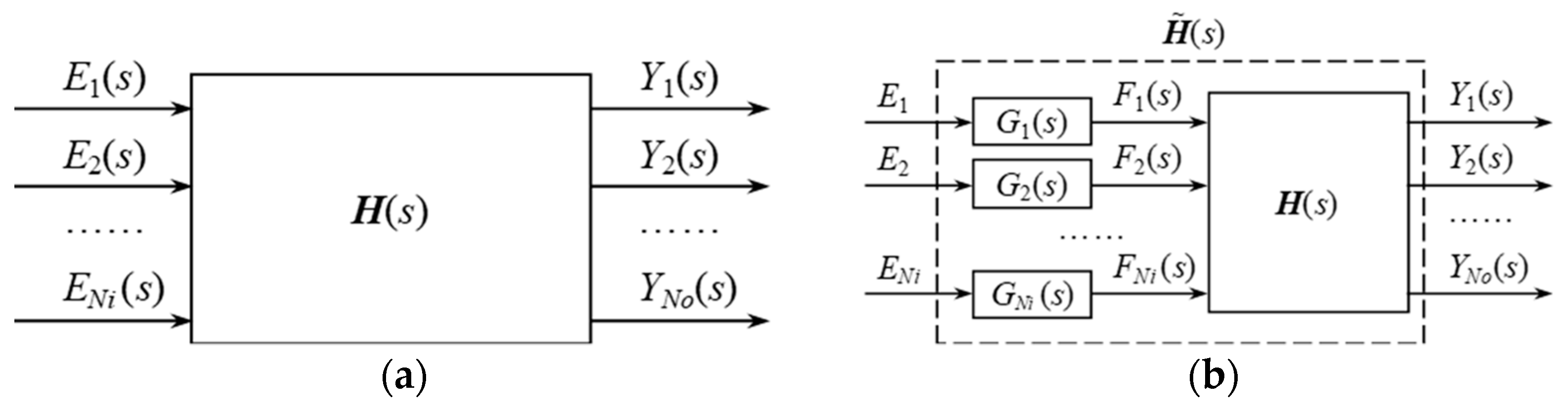
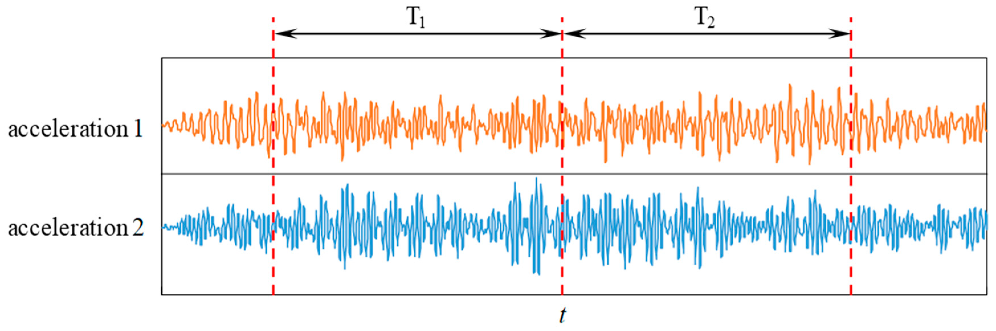
2.3. Delayed TRF Approach for Periodic False Mode Identification

The acceleration dynamic response of two DOFs in the numerical model of a multiple DOF system at time periods T₁ and T₂ is shown in Figure 2, and a set of delayed TRFs $t_{ij}^{1,2}\left(s\right)$ and $t_{ij}^{2,1}\left(s\right)$ can be constructed, defined as follows:

$$t_{ij}^{1,2}\left(s\right)=\frac{Y_i^1\left(s\right)}{Y_j^2\left(s\right)}, t_{ij}^{2,1}\left(s\right)=\frac{Y_i^2\left(s\right)}{Y_j^1\left(s\right)}$$

(22)

where $Y^1\left(s\right)$ and $Y^2\left(s\right)$ are the Laplace transformations of the acceleration response in time period 1 and time period 2, respectively; i and j are different response DOFs.

Due to the limited duration of time periods T₁ and T₂, the spectra of the periodic and random components of the system excitation during the two time periods satisfy Equations (16) and (17).

From Equations (4) and (15)–(19), when $s\to {\lambda }_m$, the following exist:

$$\begin{array}{l}\underset{s\to {\lambda }_m}{\lim }{t}_{ij}^{1,2}\left(s\right)=\frac{\underset{s\to {\lambda }_m}{\lim }{\displaystyle {\sum }_{k=1}^Q\left(s-{\lambda }_m\right)H_{ik}\left(s\right)F_k^1\left(s\right)}}{\underset{s\to {\lambda }_m}{\lim }{\displaystyle {\sum }_{k=1}^Q\left(s-{\lambda }_m\right)H_{jk}\left(s\right)F_k^2\left(s\right)}}=\frac{{\displaystyle {\sum }_{k=1}^Q{\psi }_{m,i}{l}_{m,k}\left(P_k^1\left({\lambda }_m\right)+R_k^1\left({\lambda }_m\right)\right)}}{{\displaystyle {\sum }_{k=1}^Q{\psi }_{m,j}{l}_{m,k}\left(P_k^2\left({\lambda }_m\right)+R_k^2\left({\lambda }_m\right)\right)}}\\ \hspace{1em}\hspace{1em}\hspace{1em}=\frac{{\displaystyle {\sum }_{k=1}^Q{\psi }_{m,i}{l}_{m,k}\left(0+R_k^1\left({\lambda }_m\right)\right)}}{{\displaystyle {\sum }_{k=1}^Q{\psi }_{m,j}{l}_{m,k}\left(0+R_k^2\left({\lambda }_m\right)\right)}}=\frac{{\psi }_{m,i}}{{\psi }_{m,j}}\cdot \frac{{\displaystyle {\sum }_{k=1}^Q{l}_{m,k}{R}_k^1\left({\lambda }_m\right)}}{{\displaystyle {\sum }_{k=1}^Q{l}_{m,k}{R}_k^2\left({\lambda }_m\right)}}\end{array}$$

(23)

Due to the randomness of $R^l\left(s\right)$, generally $R_k^1\left({\lambda }_m\right)\ne R_k^2\left({\lambda }_m\right)$, the delayed transmission rates at different combinations of time periods are not the same at the system’s intrinsic pole ${\lambda }_m$, i.e.,

$$t_{ij}^{1,2}\left({\lambda }_m\right)\ne t_{ij}^{2,3}\left({\lambda }_m\right)\ne \cdots \ne t_{ij}^{k-1,k}\left({\lambda }_m\right)$$

(24)

Similarly, from Equations (4) and (15)–(19), the following equation is obtained when $s\to {\gamma }_r$:

$$\begin{array}{l}\underset{s\to {\gamma }_r}{\lim }{t}_{ij}^{1,2}\left(s\right)=\frac{\underset{s\to {\gamma }_r}{\lim }{\displaystyle {\sum }_{k=1}^Q{H}_{ik}\left(s\right)F_k^1\left(s\right)}}{\underset{s\to {\gamma }_r}{\lim }{\displaystyle {\sum }_{k=1}^Q{H}_{jk}\left(s\right)F_k^2\left(s\right)}}=\frac{{\displaystyle {\sum }_{k=1}^Q{H}_{ik}\left({\gamma }_r\right)\left(P_k^1\left({\gamma }_r\right)+R_k^1\left({\gamma }_r\right)\right)}}{{\displaystyle {\sum }_{k=1}^Q{H}_{jk}\left({\gamma }_r\right)\left(P_k^2\left({\gamma }_r\right)+R_k^2\left({\gamma }_r\right)\right)}}\\ \hspace{1em}\hspace{1em}\hspace{1em}\hspace{1em}=\frac{{\displaystyle {\sum }_{k=1}^Q{H}_{ik}\left({\gamma }_r\right)\left(a_{rk}+o\left(a_{rk}\right)\right)}}{{\displaystyle {\sum }_{k=1}^Q{H}_{jk}\left({\gamma }_r\right)\left(a_{rk}+o\left(a_{rk}\right)\right)}}\approx \frac{{\displaystyle {\sum }_{k=1}^Q{a}_{rk}{H}_{ik}\left({\gamma }_r\right)}}{{\displaystyle {\sum }_{k=1}^Q{a}_{rk}{H}_{jk}\left({\gamma }_r\right)}}\end{array}$$

(25)

Analogously, it can be obtained that

$$\underset{s\to {\gamma }_r}{\lim }{t}_{ij}^{2,1}\left(s\right)\approx \frac{{\displaystyle {\sum }_{k=1}^Q{a}_{rk}{H}_{ik}\left({\gamma }_r\right)}}{{\displaystyle {\sum }_{k=1}^Q{a}_{rk}{H}_{jk}\left({\gamma }_r\right)}}$$

(26)

Comparing Equations (25) and (26), it is obtained that

$$t_{ij}^{1,2}\left({\gamma }_r\right)\approx t_{ij}^{2,1}\left({\gamma }_r\right)$$

(27)

The value of Equation (26) is independent of the selected time period, so the delayed transmissibility at each combination of time periods is approximately equal at the periodic excitation frequency ${\gamma }_r$, i.e.,

$$t_{ij}^{1,2}\left({\gamma }_r\right)\approx t_{ij}^{2,3}\left({\gamma }_r\right)\approx \cdots \approx t_{ij}^{k-1,k}\left({\gamma }_r\right)$$

(28)

It is clear that the delayed TRF $t_{ij}^{1,2}\left(s\right)$ intersects at the periodic excitation frequency ${\gamma }_r$ and varies at the natural frequency ${\lambda }_m$ of the system. The corresponding proposed frequency response function is constructed according to Equation (6), and its peak indicates only periodic false modes. Thus, by comparing the modal parameter identification results of the conventional TRF and the delayed TRF, the effective identification of the real modal parameters of the structure under periodic excitation can be achieved.

3. Example Analysis

3.1. Numerical Calculation of a 4-DOF System

3.1.1. Dynamic Response of the System

The modal parameters were identified for a 4-DOF spring-damped-mass system as shown in Figure 3. Excitations F₁ and F₂ for 100 s were applied to degrees of freedom 1 and 2, and both loads contained both random and periodic excitations, as shown in

Table 1. Two dynamic load components.

Load	F1	F2
Component 1	Periodic excitation 1 (3.1 Hz)	Periodic excitation 2 (6 Hz)
Component 2	White noise 1	White noise 1

¹ The white noise components of F₁ and F₂ are uncorrelated with each other, and the signal-to-noise ratio of the periodic component relative to the white noise is 10 dB.

. The parameters of the system were as follows: k₁~k₄ = 1000 N/m, m₁~m₄ = 1 kg, and c₁~c₄ = 0.5 N·s/m. The Newmark method was used to solve the acceleration dynamic response of the system with a sampling frequency of 200 Hz, where the acceleration responses of DOFs 3 and 4 in 40–50 s are shown in Figure 4. The overall calculation showed that the natural frequency from 1st to 4th order of the system was in the range of 0–10 Hz, so the sampling frequency satisfied Shannon’s sampling theorem ($f_s\ge 2f_{\max }$).

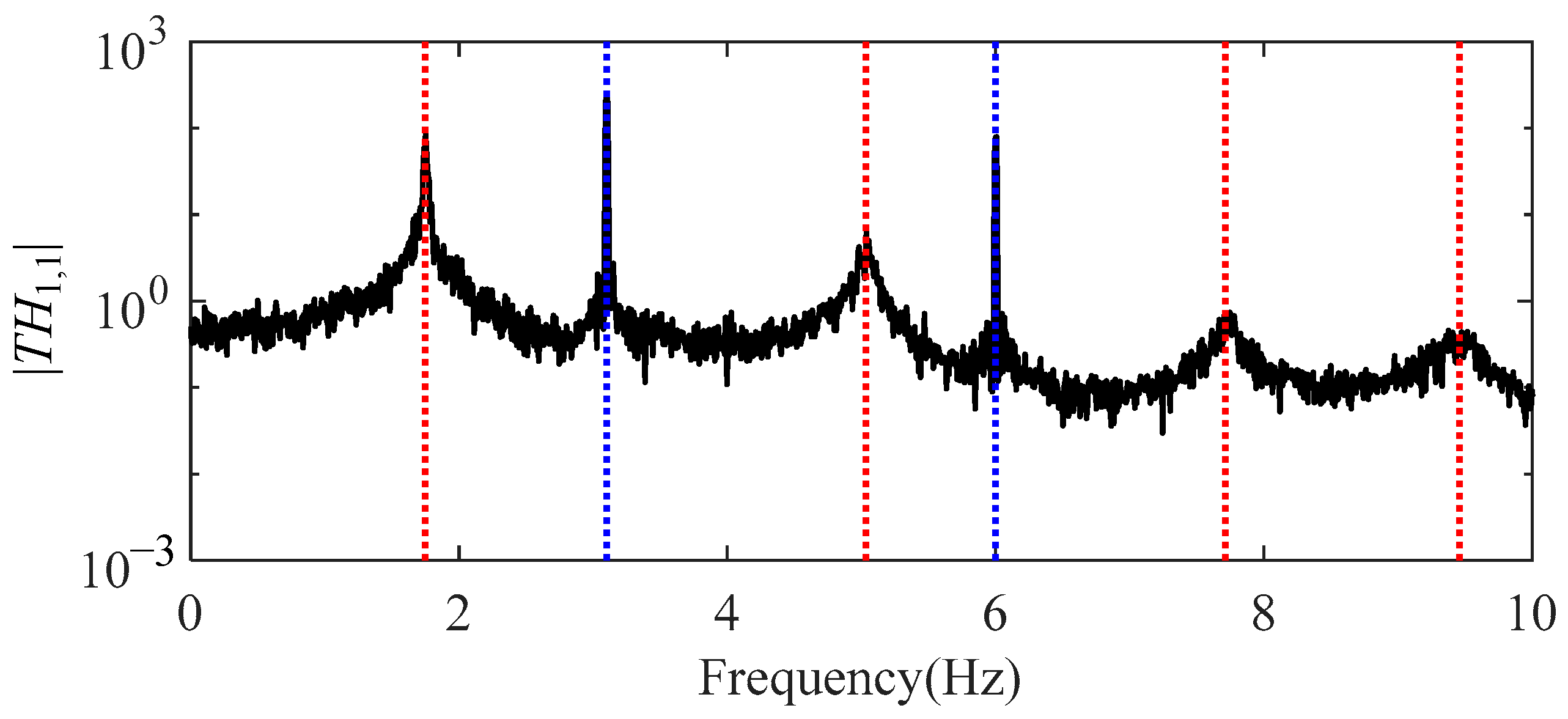
3.1.2. Modal Parameter Identification Based on TRF

The acceleration dynamic response of 100 s was divided into 20 groups of equal length, the TRF t₃₄ between DOF 3 and DOF 4 was estimated using the H_v method, and the obtained 20 groups of t₃₄ are shown in Figure 5, which is represented by a curve with random colors. The red dashed line in Figure 5 represents the theoretical value of natural frequency in each order of the system, and the blue dashed line represents the periodic frequency in the excitation. The TRFs around the above frequencies are shown in Figure 6. It can be seen that the overall TRFs of the multiple dynamic responses had significant discretion due to the random components in the excitation, but always intersected at the natural and periodic excitation frequencies of the system.

The proposed frequency response function matrix was constructed according to Equation (6); Figure 7, which contains six peaks, shows element $T{H}_{1,1}(s)$: the 4th-order intrinsic frequency peak and the 2nd-order periodic excitation peak.

The delayed TRF $t_{34}^{ij}$ (i = 1, 2, …, 19; j = i + 1) of the acceleration response of DOF 3 and DOF 4 were constructed according to Equation (18), as shown in Figure 8 and Figure 9, and it can be seen that the delayed TRFs intersected only at the periodic excitation frequency.

At the same time, the quasi-frequency response function was constructed according to Equation (6), and the pole indication curve was obtained as shown in Figure 10. At this point, only the 2nd-order frequency peak of the periodic excitation is included in Figure 10.

The peak frequencies of the two curves in Figure 7 and Figure 10 were identified; comparison of the two could accurately distinguish the natural frequency of the system, and then the true modal vibration pattern and damping ratio of the structure could be identified. The theoretical and identified values of the system modal frequencies and damping ratios are shown in

Table 2. Identification results of the modal frequency and damping ratio of the 4-DOF system.

Modal Number	Frequency (Hz)			Damping Ratio (%)
	Theoretical Value	Identified Value	Error Rate (%)	Theoretical Value	Identified Value	Error Rate (%)
1	1.748	1.750	0.10	0.27	0.28	3.70
2	5.033	5.030	−0.06	0.79	0.77	−2.53
3	7.711	7.693	−0.23	1.21	1.24	2.48
4	9.459	9.450	−0.09	1.49	1.52	2.01

, and the theoretical and identified values of the modal vibration patterns are displayed in Figure 11. These identification results show that the TRF method has high accuracy for the identification of system modal parameters.

3.1.3. Robustness Check of the Delayed TRF

The above arithmetic example confirms that the joint delayed TRF approach could effectively identify the intrinsic modal parameters of the system. Thus, considering that in some extreme cases, the periodic excitation energy is lower or closer to some natural frequencies, the following calculation example is set out in this section to test the detection effect of the periodic excitation frequency in such cases. The four sets of periodic components in the load excitation included 1.9 Hz (f_n1 + 0.15 Hz) and 7.91 Hz (f_n3 + 0.2 Hz), close to the natural frequency, and 3.1 Hz (f_n1 + 1.35 Hz) and 6 Hz (f_n2 + 0.97 Hz), far from the natural frequency. On this basis, the signal-to-noise ratios of the periodic and random components of the excitation were set to 20 dB, 0 dB, and −20 dB, representing cases of strong, moderate, and weak periodic excitation, respectively.

The conventional TRF and delayed TRF were used to establish the proposed frequency response function, respectively (Figure 12). From Figure 12, even when the intensity of the periodic component of the excitation was relatively weak or its frequency was closer to the natural frequency of the structure, the frequency of the periodic excitation could be accurately identified using the proposed frequency response function of the delayed TRF, so the method has strong robustness for identifying periodic false modes.

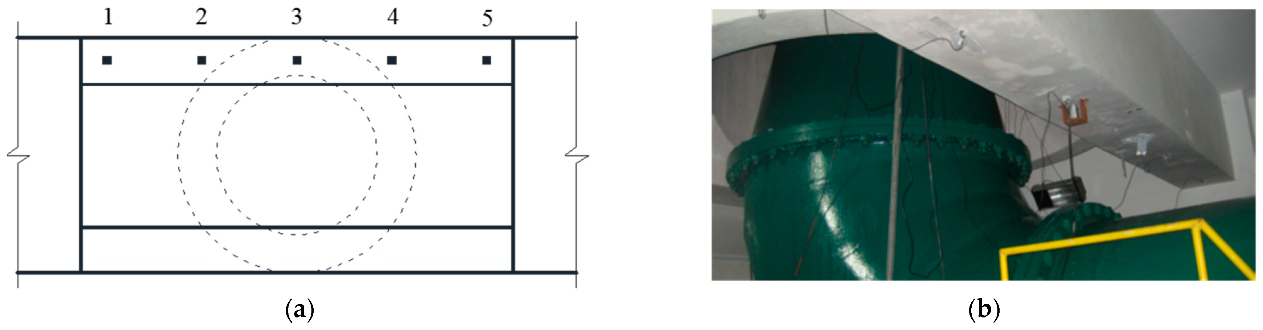
3.2. Modal Parameter Identification Example of a Pump Station Plant

The considered medium-sized pumping station adopts the vertical unit type (Figure 13) and the rated speed of the pump unit is 500 r/min. The static and dynamic loads resulting from pump operation are mainly carried by the two lower main beams. To identify the dynamic characteristics of the main beam in the vertical direction, sensors were placed on its lower part as shown in Figure 14. The acceleration response of the structure was measured under stable operation of the unit, with a sampling frequency of 1024 Hz. The acceleration response of each measurement point in 10 s is presented in Figure 15.

The quasi-frequency response was constructed using the conventional transmissibility and delayed transmissibility, as shown in Figure 16.

Comparing the poles in Figure 16a,b yielded the natural and periodic frequencies of the structured system, as shown in

Table 3. Frequency identification results of the main beam.

Frequency Type	Frequency Value (Hz)
Natural frequency	34, 43.5, 61.5
Periodic frequency	8.33, 16.67, 25, 41.7, 50, 58.3, 66.7, 83.3

. The unit rotational frequency was 8.33 Hz, which was converted from the rated speed of the pump, 500 r/min. The frequency of each periodic excitation in Table 3 is a multiple of the rotational frequency.

The FSDD method was further applied to identify the modal vibration pattern of the main beam in each order, as shown in Figure 17. The MAC indexes of the modal vibration identification results are shown in

Table 4. MAC index of modal shape recognition results.

Order of Modes	1st Order	2nd Order	3rd Order
1st order	1.000	0.005	0.001
2nd order	0.005	1.000	0.002
3rd order	0.001	0.002	1.000

, which shows that the modal vibration modes were approximately linearly independent of each other, verifying the accuracy of the modal vibration modes. The corresponding damping ratios of each order were 1.6%, 2.2%, and 2.8%. The above results show that the combined transmissibility and delayed transmissibility methods effectively identified the periodic false modes of the main beam of the pump pier and accurately identified the modal parameters of the structure.

4. Conclusions

To address the interference problem of periodic components in ambient excitation when identifying structural modal parameters, this paper proposes a method for identifying structural modal parameters based on the delayed TRF of the dynamic response, and presents a verification of the effectiveness and accuracy of the proposed method through numerical models and practical engineering calculations. The main conclusions are as follows:

Through theoretical derivation, the property was demonstrated that the delayed TRF tends to intersect at the periodic frequencies of the excitation and varies at the natural frequencies of a structure, and thus, the TRF can be used to indicate the periodic frequencies in the excitation. The joint application of the delayed TRF and the regular TRF could be used to identify the periodic false modes of the structure and thus extract the real mode parameters of the structure. The numerical calculation of the 4-DOF system confirmed that the method described in this paper can effectively eliminate the interference of periodic false modes and identify the real modal parameters of a system, and the applicability of the method was tested in the case of weak periodic excitation or periodic excitation with a frequency close to the natural frequency of the structure. Furthermore, based on the measured dynamic response data of a pump station structure, the modal parameters of the main beam of the pump pier were effectively identified.

In this study, the excitation generated by rotating mechanical equipment was simplified to ideal periodic excitation, and a modal recognition method based on the transfer rate function is proposed, which provided better recognition of the working condition of the unit’s smooth operation. However, the frequency or amplitude of the periodic excitation is constantly changing in the case of nonsmooth operating conditions, such as frequent changes in the load or input power of the unit. The effect of the periodic excitation on the identification of structural modal parameters and the effective identification method need to be further studied.

References

1. Lee, J.J.; Yun, C.B. Damage diagnosis of steel girder bridges using ambient vibration data. Eng. Struct. 2006, 28, 912–925. [Google Scholar] [CrossRef]
2. Han, J.; Zheng, P.; Wang, H. Structural modal parameter identification and damage diagnosis based on Hilbert-Huang transform. Earthq. Eng. Eng. Vib. 2014, 13, 101–111. [Google Scholar] [CrossRef]
3. Hakim, S.J.S.; Razak, H.A.; Ravanfar, S.A. Fault diagnosis on beam-like structures from modal parameters using artificial neural networks. Measurement 2015, 76, 45–61. [Google Scholar] [CrossRef]
4. Foti, D.; Giannoccaro, N.I.; Vacca, V.; Lerna, M. Structural operativity evaluation of strategic buildings through finite element (FE) models validated by operational modal analysis (OMA). Sensors 2020, 20, 3252. [Google Scholar] [CrossRef]
5. Tsuchimoto, K.; Narazaki, Y.; Spencer Jr, B.F. Development and validation of a post-earthquake safety assessment system for high-rise buildings using acceleration measurements. Mathematics 2021, 9, 1758. [Google Scholar] [CrossRef]
6. Magalhães, F.; Cunha, Á.; Caetano, E. Vibration based structural health monitoring of an arch bridge: From automated OMA to damage detection. Mech. Syst. Signal Process. 2012, 28, 212–228. [Google Scholar] [CrossRef]
7. Yan, Z.; Liu, H. SMoCo: A powerful and efficient method based on self-supervised learning for fault diagnosis of aero-engine bearing under limited data. Mathematics 2022, 10, 2796. [Google Scholar] [CrossRef]
8. Pan, C.; Ye, X.; Mei, L. Improved automatic operational modal analysis method and application to large-scale bridges. J. Bridg. Eng. 2021, 26, 04021051. [Google Scholar] [CrossRef]
9. Yan, W.J.; Zhao, M.J.; Sun, Q.; Ren, W.X. Transmissibility-based system identification for structural health monitoring: Fundamentals, approaches, and applications. Mech. Syst. Signal Process. 2019, 117, 453–482. [Google Scholar] [CrossRef]
10. Sun, Q.; Yan, W.J.; Ren, W.X.; Liu, L.L. Application of transmissibility measurements to operational modal analysis of railway, highway, and pedestrian cable-stayed bridges. Measurement 2019, 148, 106880. [Google Scholar] [CrossRef]
11. Liu, T.; Xu, H.; Ragulskis, M.; Cao, M.; Ostachowicz, W. A data-driven damage identification framework based on transmissibility function datasets and one-dimensional convolutional neural networks: Verification on a structural health monitoring benchmark structure. Sensors 2020, 20, 1059. [Google Scholar] [CrossRef] [Green Version]
12. Devriendt, C.; Guillaume, P. The use of transmissibility measurements in output-only modal analysis. Mech. Syst. Signal Process. 2007, 21, 2689–2696. [Google Scholar] [CrossRef]
13. Lage, Y.E.; Maia, N.M.M.; Neves, M.M.; Ribeiro, A.M.R. Force identification using the concept of displacement transmissibility. J. Sound Vib. 2013, 332, 1674–1686. [Google Scholar] [CrossRef]
14. Araújo, I.G.; Laier, J.E. Operational modal analysis using SVD of power spectral density transmissibility matrices. Mech. Syst. Signal Process. 2014, 46, 129–145. [Google Scholar] [CrossRef]
15. Araújo, I.D.G. Transmissibility-based operational modal analysis: Unified concept and its application. Mech. Syst. Signal Process. 2022, 178, 109302. [Google Scholar] [CrossRef]
16. Devriendt, C.; Guillaume, P. Identification of modal parameters from transmissibility measurements. J. Sound Vib. 2008, 314, 343–356. [Google Scholar] [CrossRef]
17. Devriendt, C.; De Sitter, G.; Guillaume, P. An operational modal analysis approach based on parametrically identified multivariable transmissibilities. Mech. Syst. Signal Process. 2019, 24, 1250–1259. [Google Scholar] [CrossRef]
18. Devriendt, C.; Weijtjens, W.; De Sitter, G.; Guillaume, P. Combining multiple single-reference transmissibility functions in a unique matrix formulation for operational modal analysis. Mech. Syst. Signal Process. 2013, 40, 278–287. [Google Scholar] [CrossRef]
19. Weijtjens, W.; De Sitter, G.; Devriendt, C.; Guillaume, P. Operational modal parameter estimation of MIMO systems using transmissibility functions. Automatica 2014, 50, 559–564. [Google Scholar] [CrossRef]
20. Zhang, Y.N.; Wang, T.; Xia, Z.P. Transmissibility based operational modal analysis. J. Vib. Meas. Diagn. 2015, 35, 945–949+995, (In Chinese with English abstract). [Google Scholar]
21. Araújo, I.G.; Sánchez, J.A.G.; Andersen, P. Modal parameter identification based on combining transmissibility functions and blind source separation techniques. Mech. Syst. Signal Process. 2018, 105, 276–293. [Google Scholar] [CrossRef]
22. Li, X.Z.; Dong, X.J.; Yue, X.B.; Huang, W.; Peng, Z.K. Dynamic characteristics of vibration response transmissibility and its application in operational modal analysis. J. Vib. Shock. 2019, 38, 62–70, (In Chinese with English abstract). [Google Scholar]
23. Mohanty, P.; Rixen, D.J. Operational modal analysis in the presence of harmonic excitation. J. Sound Vib. 2004, 270, 93–109. [Google Scholar] [CrossRef]
24. Mohanty, P.; Rixen, D.J. Modified ERA method for operational modal analysis in the presence of harmonic excitations. Mech. Syst. Sign. Process. 2006, 20, 114–130. [Google Scholar] [CrossRef]
25. He, X.H.; Hua, X.G.; Chen, Z.Q.; Huang, F.L. EMD-based random decrement technique for modal parameter identification of an existing railway bridge. Eng. Struct. 2011, 33, 1348–1356. [Google Scholar] [CrossRef]
26. Carden, E.P.; Brownjohn, J.M. Fuzzy clustering of stability diagrams for vibration-based structural health monitoring. Comput. Aided Civ. Infrastruct. Eng. 2008, 23, 360–372. [Google Scholar] [CrossRef]
27. Lian, J.; Li, H.; Zhang, J. ERA modal identification method for hydraulic structures based on order determination and noise reduction of singular entropy. Sci. China Ser. E Technol. Sci. 2009, 52, 400–412. [Google Scholar] [CrossRef]
28. Dong, X.; Lian, J.; Yang, M.; Wang, H. Operational modal identification of offshore wind turbine structure based on modified stochastic subspace identification method considering harmonic interference. J. Renew. Sustain. Energy 2014, 6, 033128. [Google Scholar] [CrossRef]
29. Heylen, W.; Lammens, S.; Sas, P. Modal Analysis Theory and Testing; Katholieke Universiteit Leuven: Leuven, Belgium, 1997; Volume 200. [Google Scholar]
30. Zhang, L.M.; Wang, T.; Tamura, Y. A frequency-spatial domain decomposition (FSDD) method for operational modal analysis. Mech. Syst. Signal Process. 2010, 24, 1227–1239. [Google Scholar] [CrossRef]
31. Pintelon, R.; Schoukens, J. System Identification: A Frequency Domain Approach; John Wiley & Sons: Hoboken, NJ, USA, 2012. [Google Scholar]
Figure 1. Input–output relation diagram of two types of structure: (a) random excitation; (b) contains periodic excitation.
Mathematics 11 01019 g001
Figure 2. Acceleration responses of measurement points in different time periods.
Mathematics 11 01019 g002
Figure 3. Four-degree-of-freedom spring-damping-mass system.
Mathematics 11 01019 g003
Figure 4. Acceleration dynamic response of the system. (a) DOF 3; (b) DOF 4.
Mathematics 11 01019 g004
Figure 5. Transmissibility t34 of response in a finite time period (20 groups).
Mathematics 11 01019 g005
Figure 6. TRFs near each characteristic frequency. (a) Natural frequency 1; (b) natural frequency 2; (c) natural frequency 3; (d) natural frequency 4; (e) excitation frequency 1; (f) excitation frequency 2.
Mathematics 11 01019 g006
Figure 7. Natural frequency indication curve of T H 1 , 1 ( s ) .
Mathematics 11 01019 g007
Figure 8. Delayed TRF t 34 i j of response in a finite time period (19 groups).
Mathematics 11 01019 g008
Figure 9. Local delayed TRF. (a) Excitation frequency 1; (b) excitation frequency 2.
Mathematics 11 01019 g009
Figure 10. Natural frequency indication curve based on delayed transmissibility.
Mathematics 11 01019 g010
Figure 11. Identification results of the modal vibration pattern. (a) 1st order; (b) 2nd order; (c) 3rd order; (d) 4th order.
Mathematics 11 01019 g011
Figure 12. The virtual frequency response function with different period excitation amplitudes. (a) Conventional transmissibility (SNR = 20 dB); (b) delayed transmissibility (SNR = 20 dB); (c) conventional transmissibility (SNR = 0 dB); (d) delayed transmissibility (SNR = 0 dB); (e) conventional transmissibility (SNR = −20 dB); (f) delayed transmissibility (SNR = −20 dB).
Mathematics 11 01019 g012
Figure 13. Schematic diagram of the pumping unit of a medium-sized pumping station.
Mathematics 11 01019 g013
Figure 14. Arrangement of measuring points of the main beam of the pier base. (a) Diagram of measuring point arrangement; (b) upstream-side main beam acceleration measurement point.
Mathematics 11 01019 g014
Figure 15. Acceleration response of each measurement point. (a) Measurement point 1; (b) measurement point 2; (c) measurement point 3; (d) measurement point 4; (e) measurement point 5.
Mathematics 11 01019 g015
Figure 16. System pole recognition based on the virtual frequency response function. (a) Conventional TRF; (b) delayed TRF.
Mathematics 11 01019 g016
Figure 17. Identification results of vibration modes of the main beam. (a) 1st order; (b) 2nd order; (c) 3rd order.
Mathematics 11 01019 g017